chapter 11testbankeasy.eu/sample/solution manual for managerial... · web viewfull file at...
TRANSCRIPT
Full file at http://testbankeasy.eu/Solution-Manual-for-Managerial-Accounting,-15th-Edition---GarrisonChapter 10Standard Costs and Variances
Solutions to Questions
10-1 A quantity standard indicates how much of an input should be used to make a unit of output. A price standard indicates how much the input should cost.
10-2 Separating an overall variance into a price variance and a quantity variance provides more information. Moreover, price and quantity variances are usually the responsibilities of different managers.
10-3 The materials price variance is usually the responsibility of the purchasing manager. The materials quantity and labor efficiency variances are usually the responsibility of production managers and supervisors.
10-4 The materials price variance can be computed either when materials are purchased or when they are placed into production. It is usually better to compute the variance when materials are purchased because that is when the purchasing manager, who has responsibility for this variance, has completed his or her work. In addition, recognizing the price variance when materials are purchased allows the company to carry its raw materials in the inventory accounts at standard cost, which greatly simplifies bookkeeping.
10-5 This combination of variances may indicate that inferior quality materials were purchased at a discounted price, but the low-quality materials created production problems.
10-6 If standards are used to find who to blame for problems, they can breed resentment and undermine morale.
Standards should not be used to find someone to blame for problems.
10-7 Several factors other than the contractual rate paid to workers can cause a labor rate variance. For example, skilled workers with high hourly rates of pay can be given duties that require little skill and that call for low hourly rates of pay, resulting in an unfavorable rate variance. Or unskilled or untrained workers can be assigned to tasks that should be filled by more skilled workers with higher rates of pay, resulting in a favorable rate variance. Unfavorable rate variances can also arise from overtime work at premium rates.
10-8 If poor quality materials create production problems, a result could be excessive labor time and therefore an unfavorable labor efficiency variance. Poor quality materials would not ordinarily affect the labor rate variance.
10-9 If overhead is applied on the basis of direct labor-hours, then the variable overhead efficiency variance and the direct labor efficiency variance will always be favorable or unfavorable together. Both variances are computed by comparing the number of direct labor-hours actually worked to the standard hours allowed. That is, in each case the formula is:
Efficiency variance = SR(AH – SH)Only the “SR” part of the formula, the standard rate, differs between the two variances.
10-10 If labor is a fixed cost and standards are tight, then the only way to generate favorable labor efficiency
full file at http://testbankeasy.com
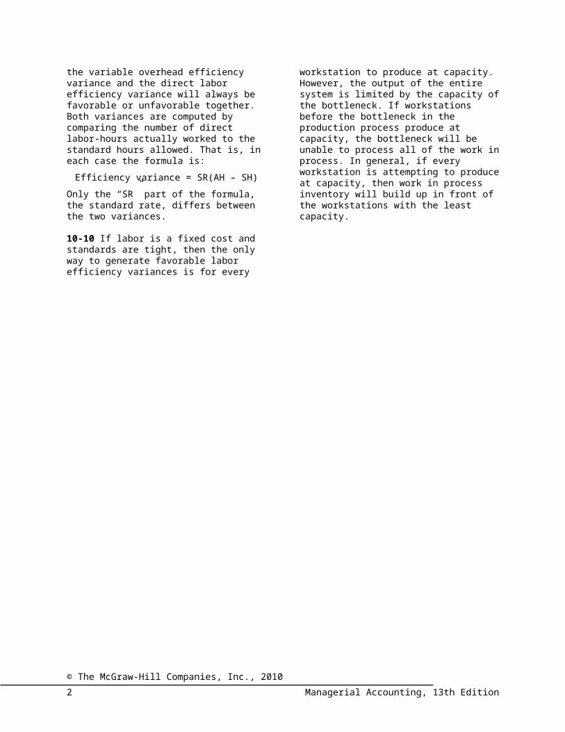
variances is for every workstation to produce at capacity. However, the output of the entire system is limited by the capacity of the bottleneck. If workstations before the bottleneck in the production process produce at capacity, the bottleneck will be unable to process all of the work in process. In general, if every
workstation is attempting to produce at capacity, then work in process inventory will build up in front of the workstations with the least capacity.
© The McGraw-Hill Companies, Inc., 20102 Managerial Accounting, 13th Edition
The Foundational 15
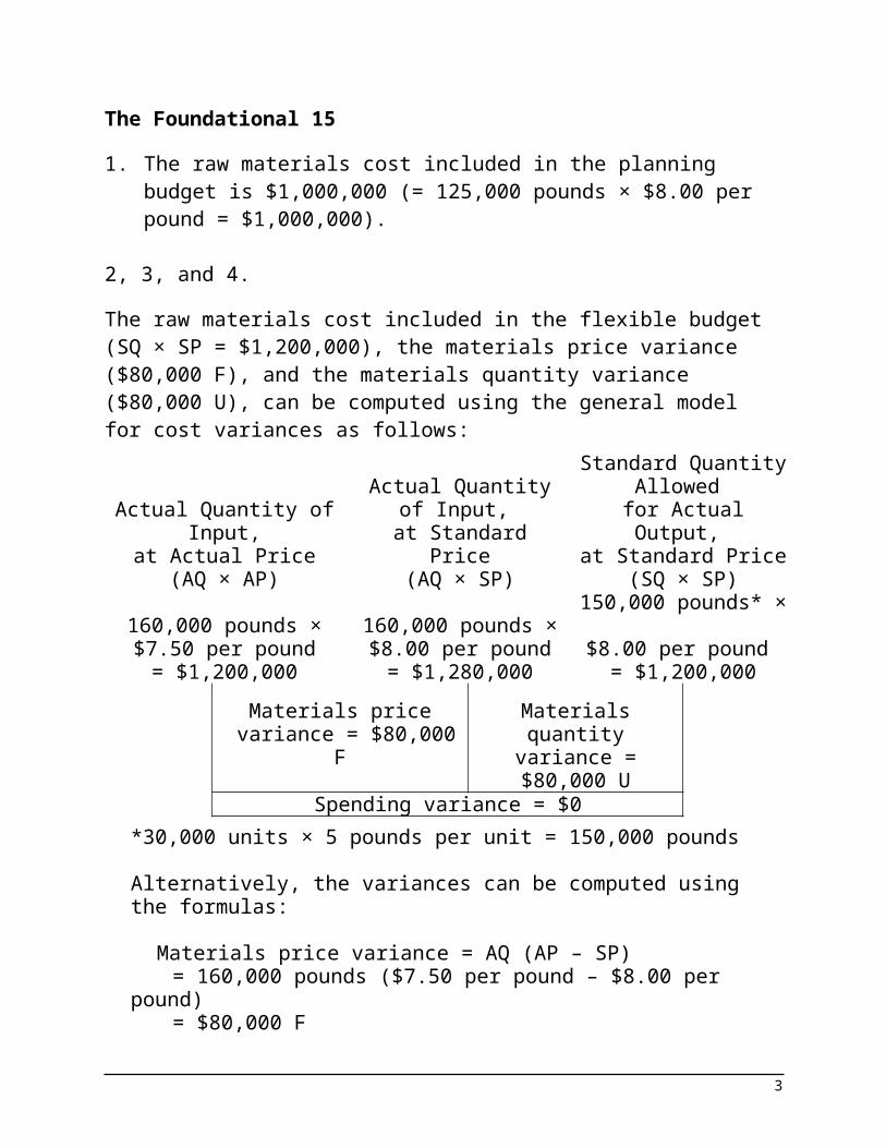
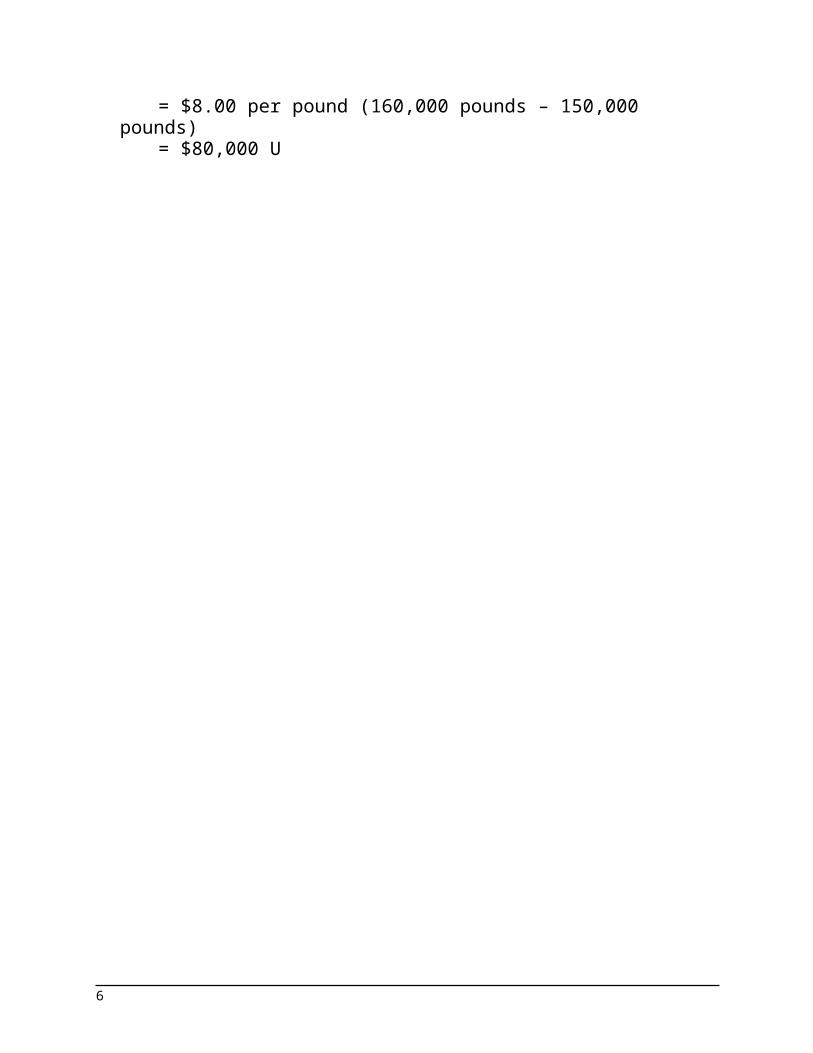
1. The raw materials cost included in the planning budget is $1,000,000 (= 125,000 pounds × $8.00 per pound = $1,000,000).
2, 3, and 4.The raw materials cost included in the flexible budget (SQ × SP = $1,200,000), the materials price variance ($80,000 F), and the materials quantity variance ($80,000 U), can be computed using the general model for cost variances as follows:
Actual Quantity of Input,
at Actual Price(AQ × AP)
Actual Quantity of Input,
at Standard Price(AQ × SP)
Standard Quantity Allowed
for Actual Output, at Standard Price
(SQ × SP)160,000 pounds × $7.50 per pound
= $1,200,000
160,000 pounds ×$8.00 per pound
= $1,280,000
150,000 pounds* × $8.00 per pound
= $1,200,000Materials price
variance = $80,000 FMaterials quantity
variance = $80,000 U
Spending variance = $0*30,000 units × 5 pounds per unit = 150,000 pounds
Alternatively, the variances can be computed using the formulas:
Materials price variance = AQ (AP – SP)= 160,000 pounds ($7.50 per pound – $8.00 per pound)= $80,000 F
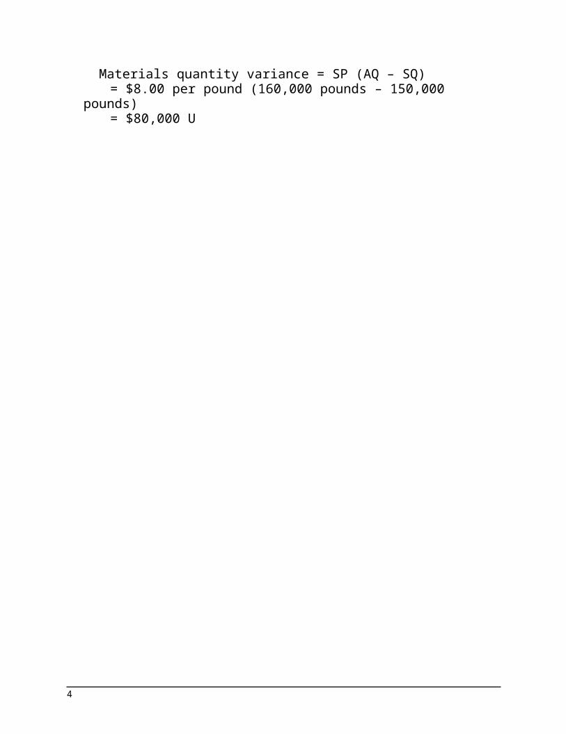
Materials quantity variance = SP (AQ – SQ)= $8.00 per pound (160,000 pounds – 150,000 pounds)= $80,000 U
3
The Foundational 15 (continued)
5. and 6.The materials price variance ($85,000 F) and the materials quantity variance ($80,000 U) can be computed as follows:
Actual Quantityof Input,
at Actual Price(AQ × AP)
Actual Quantityof Input,
at Standard Price(AQ × SP)
Standard Quantity Allowed for Actual
Output,at Standard Price
(SQ × SP)170,000 pounds × $7.50 per pound
= $1,275,000
170,000 pounds × $8.00 per pound
= $1,360,000
150,000 pounds* × $8.00 per pound
= $1,200,000Materials price
variance = $85,000 F
160,000 pounds × $8.00 per pound
= $1,280,000Materials quantity
variance = $80,000 U
*30,000 units × 5 pounds per unit = 150,000 units
Alternatively, the variances can be computed using the formulas:
Materials price variance = AQ (AP – SP)= 170,000 pounds ($7.50 per pound – $8.00 per pound)= $85,000 F
Materials quantity variance = SP (AQ – SQ)= $8.00 per pound (160,000 pounds – 150,000 pounds)= $80,000 U
4

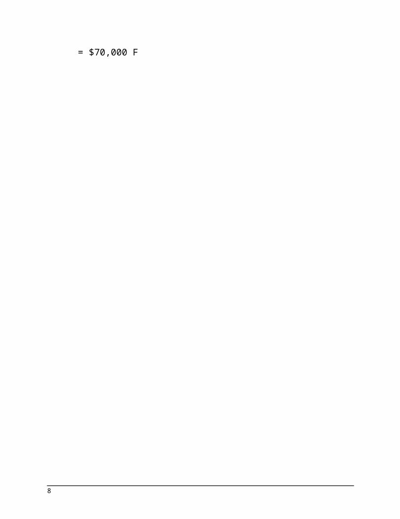
The Foundational 15 (continued)7. The direct labor cost included in the planning budget is
$700,000 (= 50,000 hours × $14.00 per hour = $700,000).
8, 9, 10, and 11.The direct labor cost included in the flexible budget (SH × SR = $840,000), the labor rate variance ($55,000 U), the labor efficiency variance ($70,000 F), and the labor spending variance ($15,000 F) can be computed using the general model for cost variances as follows:
Actual Hours of Input, at Actual Rate
(AH × AR)
Actual Hours of Input,
at Standard Rate(AH × SR)
Standard Hours Allowed
for Actual Output, at Standard Rate
(SH × SR)55,000 hours ×
$15 per hour= $825,000
55,000 hours ×$14.00 per hour
= $770,000
60,000 hours* ×$14.00 per hour
= $840,000
Labor rate variance = $55,000 U
Labor efficiency variance
= $70,000 FSpending variance = $15,000 F
*30,000 units × 2.0 hours per unit = 60,000 hours
Alternatively, the variances can be computed using the formulas:
Labor rate variance = AH (AR – SR)= 55,000 hours ($15.00 per hour – $14.00 per hour)= $55,000 U
Labor efficiency variance = SR (AH – SH)= $14.00 per hour (55,000 hours – 60,000 hours)= $70,000 F
5
The Foundational 15 (continued)
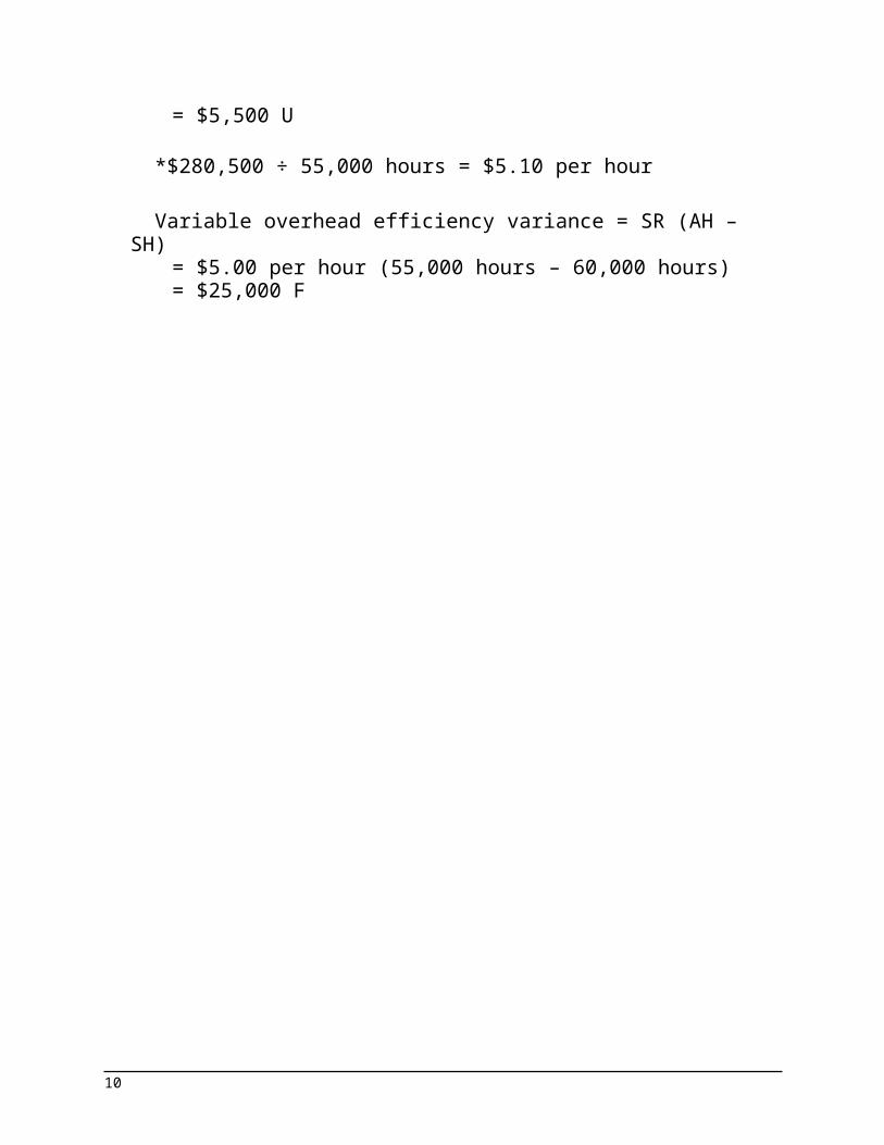
12. The variable manufacturing overhead cost included in the planning budget is $250,000 (= 50,000 hours × $5.00 per hour = $250,000).
13, 14, and 15.The variable overhead cost included in the flexible budget (SH × SR = $300,000), the variable overhead rate variance ($55,000 U), and the variable overhead efficiency variance ($25,000 F) can be computed using the general model for cost variances as follows:
Actual Hours of Input, at Actual Rate
(AH × AR)
Actual Hours of Input,
at Standard Rate(AH × SR)
Standard Hours Allowed
for Actual Output, at Standard Rate
(SH × SR)55,000 hours ×
$5.10 per hour**= $280,500
55,000 hours ×$5.00 per hour
= $275,000
60,000 hours* ×$5.00 per hour
= $300,000
Variable overhead rate variance = $5,500 U
Variable overhead efficiency variance
= $25,000 FSpending variance = $19,500 F
*30,000 units × 2.0 hours per unit = 60,000 hours** $280,500 ÷ 55,000 hours = $5.10 per hour
Alternatively, the variances can be computed using the formulas:
Variable overhead rate variance = AH (AR* – SR)= 55,000 hours ($5.10 per hour – $5.00 per hour)= $5,500 U
*$280,500 ÷ 55,000 hours = $5.10 per hour
Variable overhead efficiency variance = SR (AH – SH)= $5.00 per hour (55,000 hours – 60,000 hours)
6

= $25,000 F
7
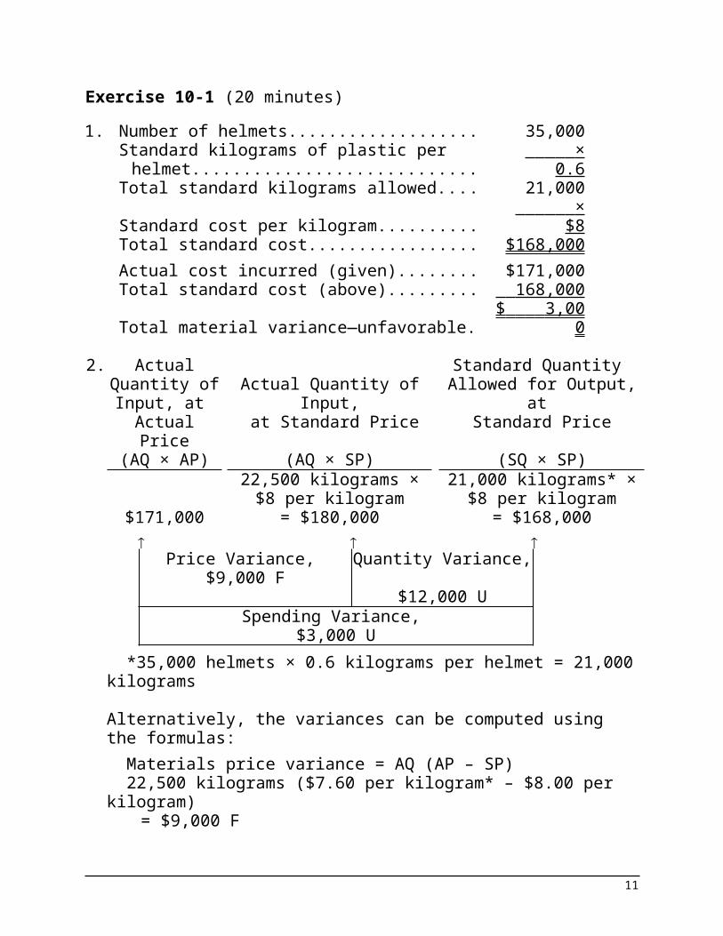
Exercise 10-1 (20 minutes)1. Number of helmets...................................... 35,000
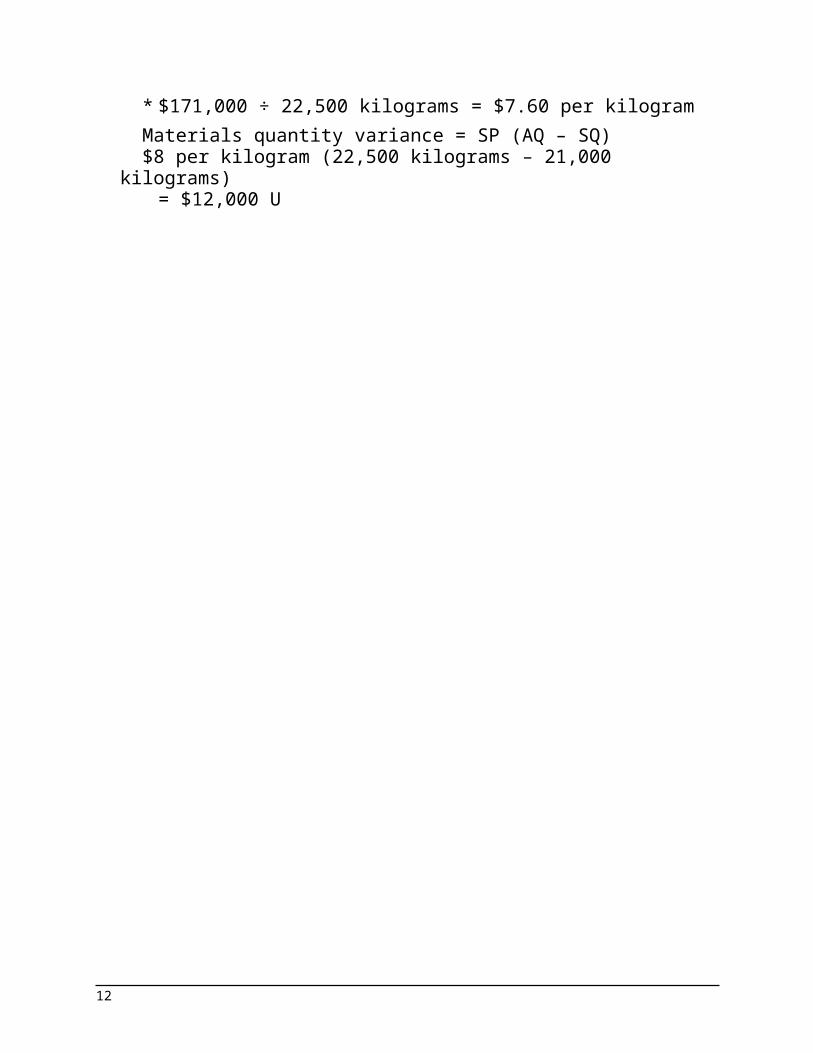
Standard kilograms of plastic per helmet.... × 0.6 Total standard kilograms allowed............... 21,000Standard cost per kilogram......................... × $8 Total standard cost..................................... $168,000Actual cost incurred (given)........................ $171,000Total standard cost (above)........................ 168,000 Total material variance—unfavorable......... $ 3,000
2. Actual Quantity of Input, at
Actual Price
Actual Quantity of Input, at Standard Price
Standard Quantity Allowed for Output, at
Standard Price
(AQ × AP) (AQ × SP) (SQ × SP)22,500 kilograms × 21,000 kilograms* ×
$8 per kilogram $8 per kilogram$171,000 = $180,000 = $168,000
Price Variance, $9,000 F
Quantity Variance, $12,000 U
Spending Variance, $3,000 U
*35,000 helmets × 0.6 kilograms per helmet = 21,000 kilograms
Alternatively, the variances can be computed using the formulas:
Materials price variance = AQ (AP – SP)22,500 kilograms ($7.60 per kilogram* – $8.00 per kilogram)
= $9,000 F* $171,000 ÷ 22,500 kilograms = $7.60 per kilogramMaterials quantity variance = SP (AQ – SQ)$8 per kilogram (22,500 kilograms – 21,000 kilograms)
= $12,000 U
8

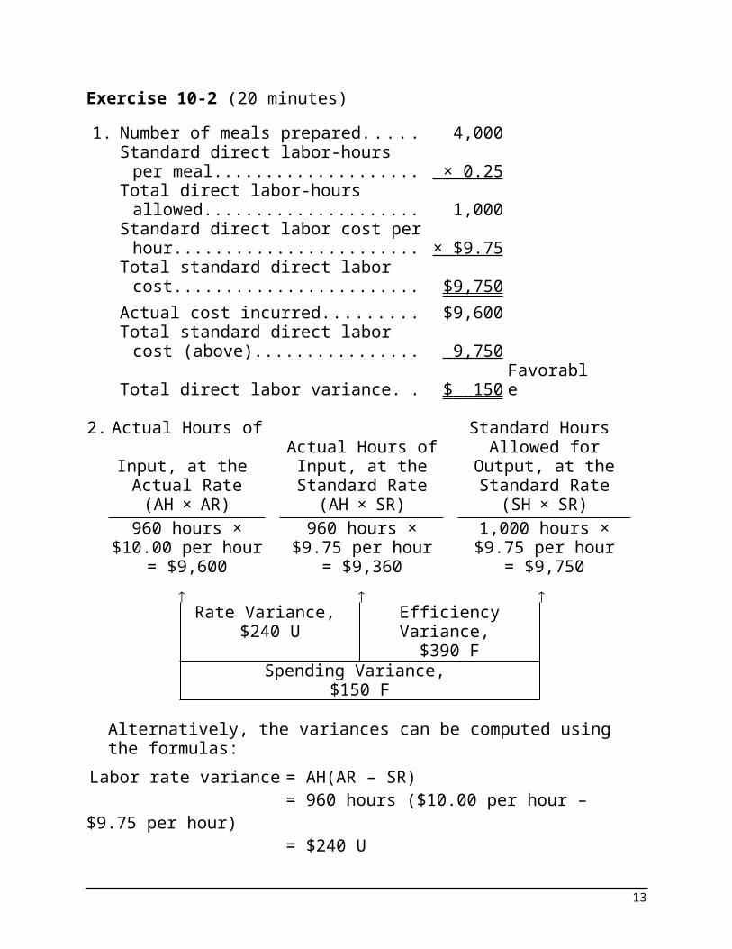
Exercise 10-2 (20 minutes)1. Number of meals prepared............. 4,000
Standard direct labor-hours per meal.............................................. × 0.25
Total direct labor-hours allowed...... 1,000Standard direct labor cost per hour × $9.75Total standard direct labor cost...... $9,750Actual cost incurred........................ $9,600Total standard direct labor cost
(above)......................................... 9,750 Total direct labor variance.............. $ 150 Favorable
2. Actual Hours of Input, at the Actual Rate
Actual Hours of Input, at the
Standard Rate
Standard Hours Allowed for Output,
at the Standard Rate
(AH×AR) (AH×SR) (SH×SR)960 hours ×
$10.00 per hour960 hours ×
$9.75 per hour1,000 hours ×$9.75 per hour
= $9,600 = $9,360 = $9,750
Rate Variance, $240 U
Efficiency Variance, $390 F
Spending Variance, $150 F
Alternatively, the variances can be computed using the formulas:Labor rate variance = AH(AR – SR)
= 960 hours ($10.00 per hour – $9.75 per hour)
= $240 ULabor efficiency variance = SR(AH – SH)
= $9.75 per hour (960 hours – 1,000 hours)
= $390 F
9
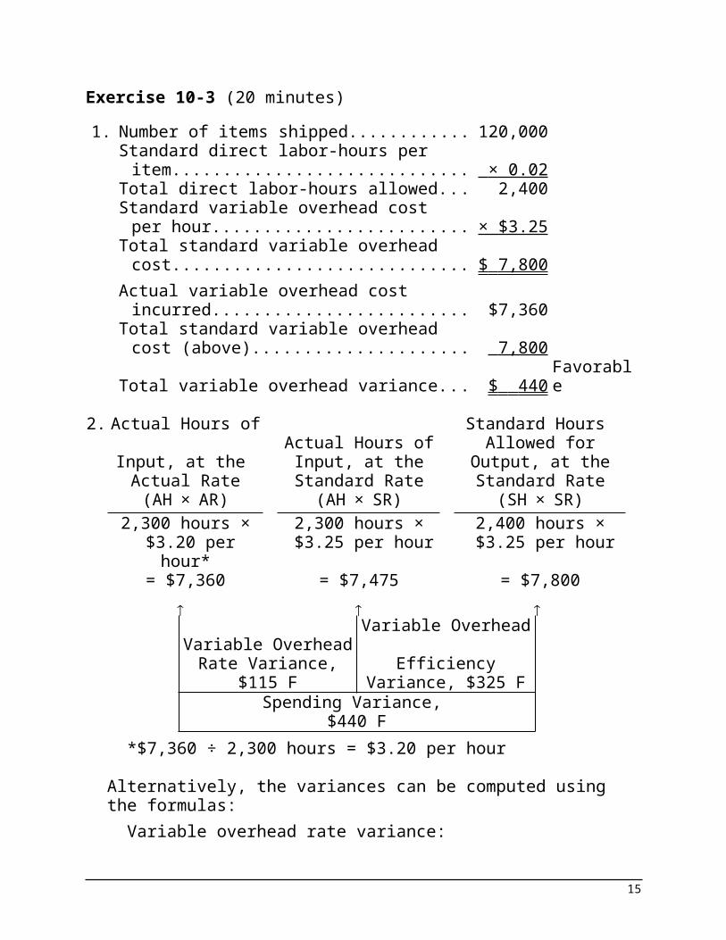
Exercise 10-3 (20 minutes)1. Number of items shipped.......................... 120,000
Standard direct labor-hours per item........ × 0.02 Total direct labor-hours allowed................ 2,400Standard variable overhead cost per
hour........................................................ × $3.25Total standard variable overhead cost...... $ 7,800 Actual variable overhead cost incurred..... $7,360Total standard variable overhead cost
(above)................................................... 7,800 Total variable overhead variance.............. $ 440 Favorable
2. Actual Hours of Input, at the Actual Rate
Actual Hours of Input, at the
Standard Rate
Standard Hours Allowed for Output,
at the Standard Rate
(AH×AR) (AH×SR) (SH×SR)2,300 hours ×
$3.20 per hour*2,300 hours × $3.25 per hour
2,400 hours × $3.25 per hour
= $7,360 = $7,475 = $7,800
Variable Overhead Rate Variance, $115
F
Variable Overhead Efficiency Variance,
$325 F
Spending Variance, $440 F
*$7,360 ÷ 2,300 hours = $3.20 per hour
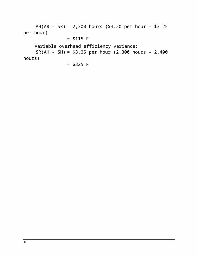
Alternatively, the variances can be computed using the formulas:
Variable overhead rate variance:AH(AR – SR) = 2,300 hours ($3.20 per hour – $3.25 per
hour)= $115 F
Variable overhead efficiency variance:SR(AH – SH) = $3.25 per hour (2,300 hours – 2,400 hours)
10
= $325 F
11
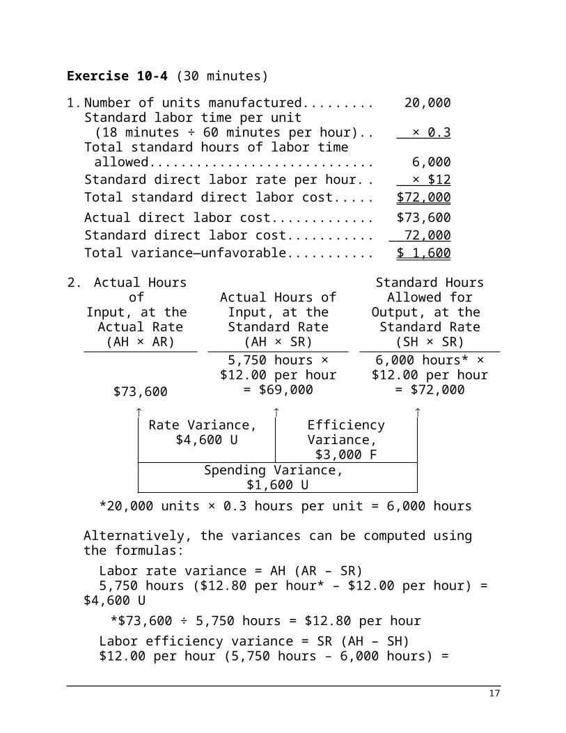
Exercise 10-4 (30 minutes)1. Number of units manufactured...................... 20,000
Standard labor time per unit (18 minutes ÷ 60 minutes per hour)........... × 0.3
Total standard hours of labor time allowed.... 6,000Standard direct labor rate per hour............... × $12 Total standard direct labor cost..................... $72,000Actual direct labor cost.................................. $73,600Standard direct labor cost............................. 72,000 Total variance—unfavorable.......................... $ 1,600
2. Actual Hours of Input, at the Actual Rate
Actual Hours of Input, at the
Standard Rate
Standard Hours Allowed for Output,
at the Standard Rate
(AH × AR) (AH × SR) (SH × SR)5,750 hours ×
$12.00 per hour6,000 hours* ×$12.00 per hour
$73,600 = $69,000 = $72,000
Rate Variance, $4,600 U
Efficiency Variance, $3,000 F
Spending Variance, $1,600 U
*20,000 units × 0.3 hours per unit = 6,000 hours
Alternatively, the variances can be computed using the formulas:
Labor rate variance = AH (AR – SR)5,750 hours ($12.80 per hour* – $12.00 per hour) = $4,600 U
*$73,600 ÷ 5,750 hours = $12.80 per hourLabor efficiency variance = SR (AH – SH) $12.00 per hour (5,750 hours – 6,000 hours) = $3,000 F
12
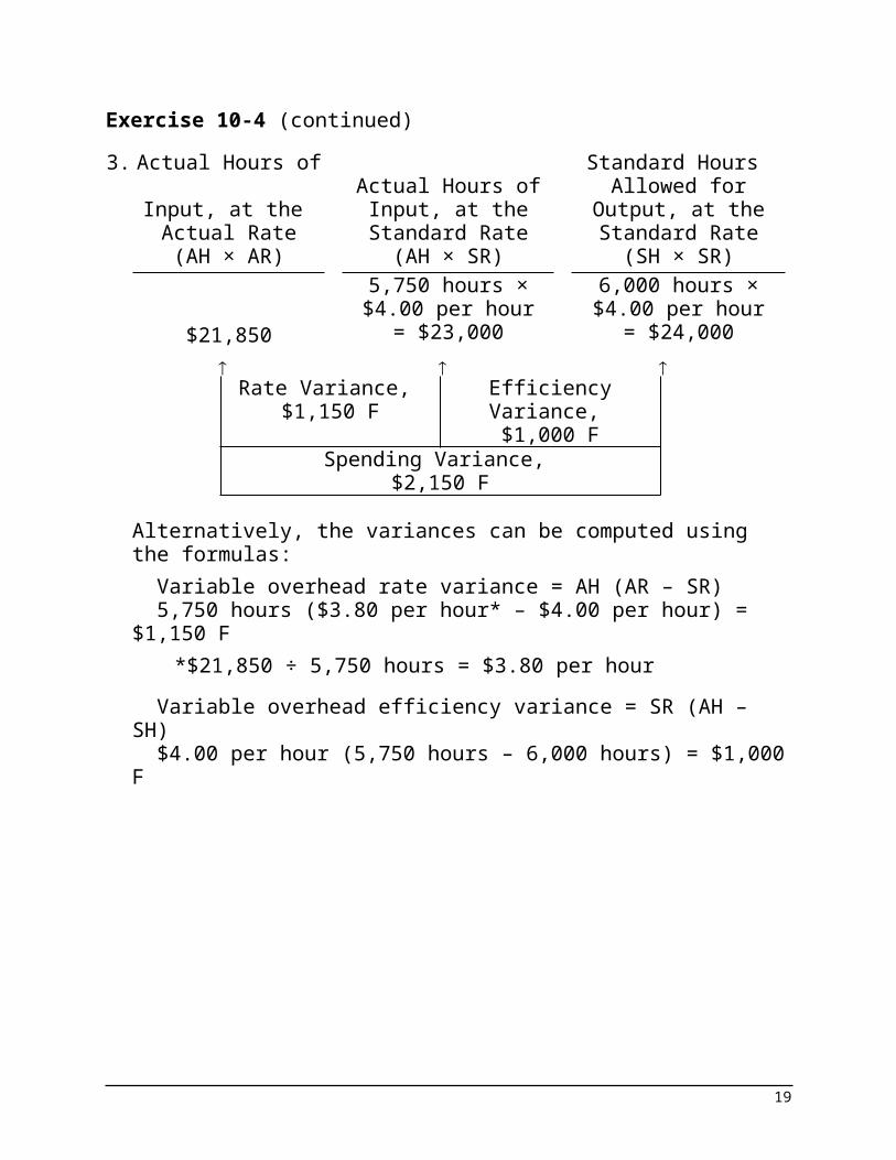
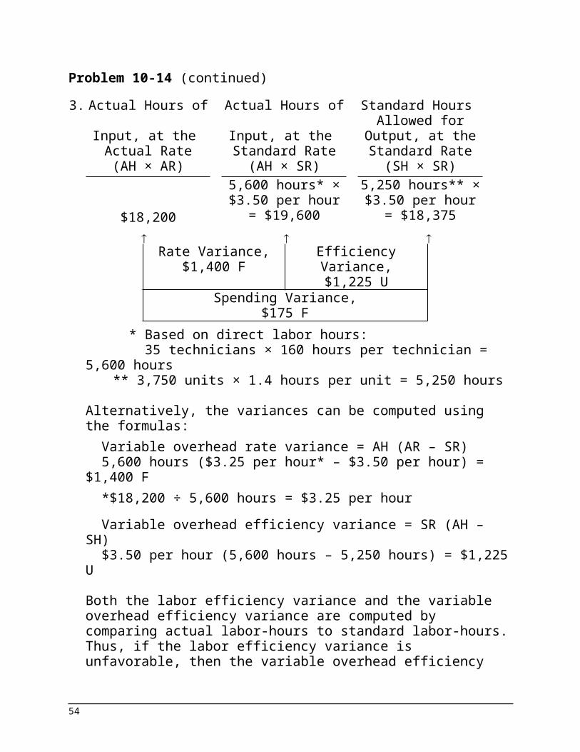
Exercise 10-4 (continued)3. Actual Hours of
Input, at the Actual Rate
Actual Hours of Input, at the
Standard Rate
Standard Hours Allowed for Output,
at the Standard Rate
(AH × AR) (AH × SR) (SH × SR)5,750 hours ×$4.00 per hour
6,000 hours ×$4.00 per hour
$21,850 = $23,000 = $24,000
Rate Variance, $1,150 F
Efficiency Variance, $1,000 F
Spending Variance, $2,150 F
Alternatively, the variances can be computed using the formulas:
Variable overhead rate variance = AH (AR – SR)5,750 hours ($3.80 per hour* – $4.00 per hour) = $1,150 F
*$21,850 ÷ 5,750 hours = $3.80 per hourVariable overhead efficiency variance = SR (AH – SH)$4.00 per hour (5,750 hours – 6,000 hours) = $1,000 F
13

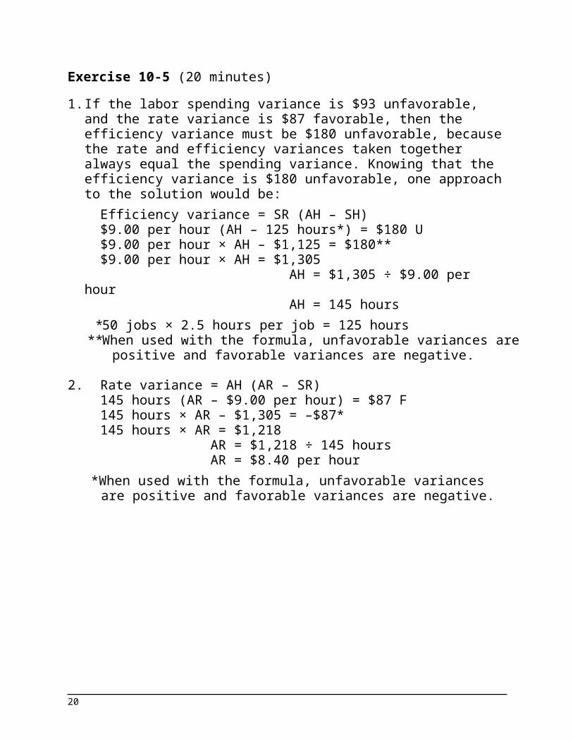
Exercise 10-5 (20 minutes)1. If the labor spending variance is $93 unfavorable, and the rate
variance is $87 favorable, then the efficiency variance must be $180 unfavorable, because the rate and efficiency variances taken together always equal the spending variance. Knowing that the efficiency variance is $180 unfavorable, one approach to the solution would be:
Efficiency variance = SR (AH – SH)$9.00 per hour (AH – 125 hours*) = $180 U$9.00 per hour × AH – $1,125 = $180**$9.00 per hour × AH = $1,305 AH = $1,305 ÷ $9.00 per hour AH = 145 hours*50 jobs × 2.5 hours per job = 125 hours
**When used with the formula, unfavorable variances are positive and favorable variances are negative.
2. Rate variance = AH (AR – SR)145 hours (AR – $9.00 per hour) = $87 F145 hours × AR – $1,305 = –$87*145 hours × AR = $1,218 AR = $1,218 ÷ 145 hours AR = $8.40 per hour
*When used with the formula, unfavorable variances are positive and favorable variances are negative.
14
Exercise 10-5 (continued)An alternative approach would be to work from known to unknown data in the columnar model for variance analysis:
Actual Hours of Input, at the Actual
Rate
Actual Hours of Input, at the
Standard Rate
Standard Hours Allowed for Output,
at the Standard Rate
(AH × AR) (AH × SR) (SH × SR)145 hours ×
$8.40 per hour145 hours ×
$9.00 per hour*125 hours§ ×
$9.00 per hour*= $1,218 = $1,305 = $1,125
Rate Variance,
$87 F*Efficiency Variance,
$180 USpending Variance,
$93 U*§50 tune-ups* × 2.5 hours per tune-up* = 125 hours*Given
15
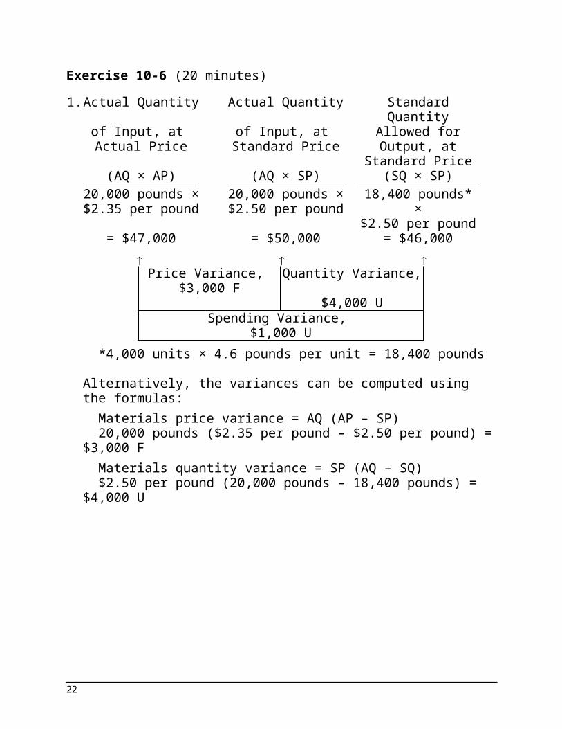
Exercise 10-6 (20 minutes)1. Actual Quantity
of Input, at Actual Price
Actual Quantity of Input, at
Standard Price
Standard Quantity Allowed
for Output, at Standard Price
(AQ × AP) (AQ × SP) (SQ × SP)20,000 pounds ×$2.35 per pound
20,000 pounds ×$2.50 per pound
18,400 pounds* ×
$2.50 per pound= $47,000 = $50,000 = $46,000
Price Variance,
$3,000 FQuantity Variance,
$4,000 USpending Variance,
$1,000 U*4,000 units × 4.6 pounds per unit = 18,400 pounds
Alternatively, the variances can be computed using the formulas:
Materials price variance = AQ (AP – SP)20,000 pounds ($2.35 per pound – $2.50 per pound) =
$3,000 FMaterials quantity variance = SP (AQ – SQ)$2.50 per pound (20,000 pounds – 18,400 pounds) = $4,000
U
16
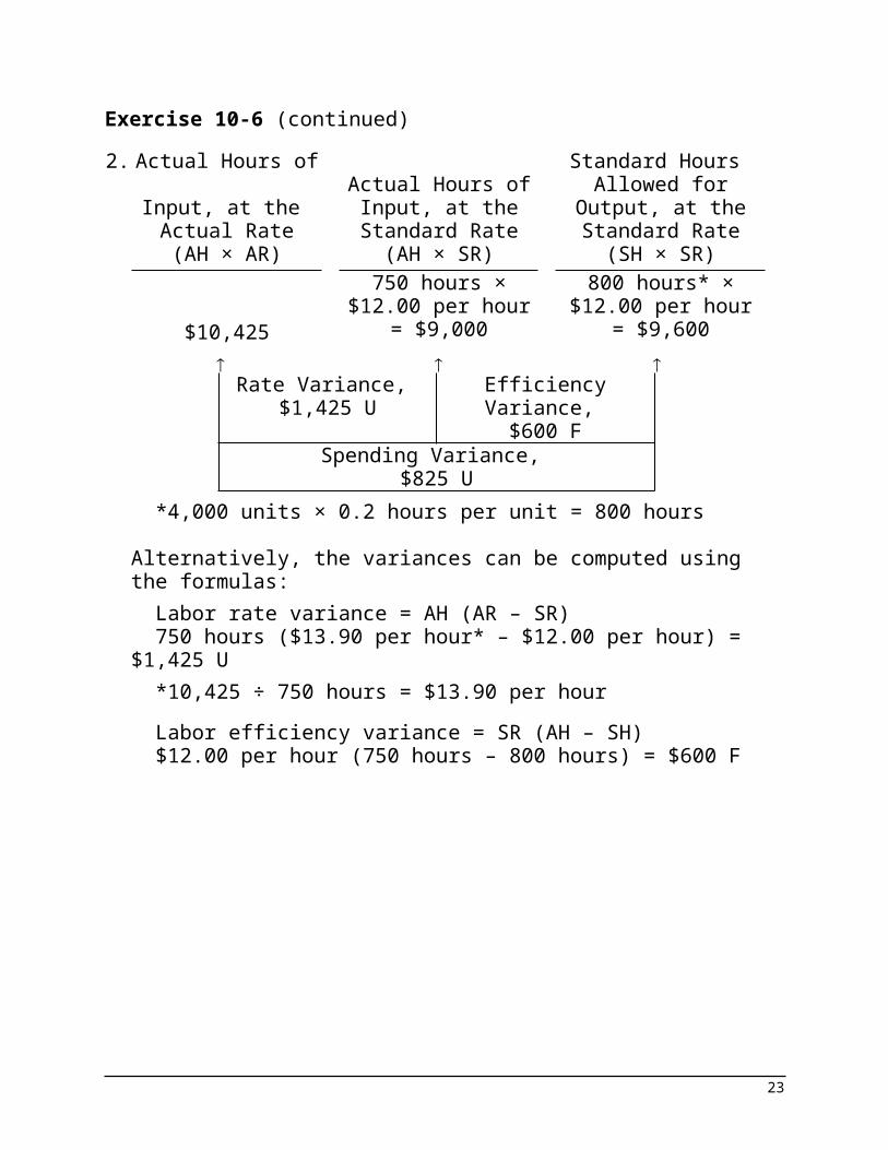
Exercise 10-6 (continued)2. Actual Hours of
Input, at the Actual Rate
Actual Hours of Input, at the
Standard Rate
Standard Hours Allowed for Output,
at the Standard Rate
(AH × AR) (AH × SR) (SH × SR)750 hours ×
$12.00 per hour800 hours* ×
$12.00 per hour$10,425 = $9,000 = $9,600
Rate Variance,
$1,425 UEfficiency Variance,
$600 FSpending Variance,
$825 U*4,000 units × 0.2 hours per unit = 800 hours
Alternatively, the variances can be computed using the formulas:
Labor rate variance = AH (AR – SR)750 hours ($13.90 per hour* – $12.00 per hour) = $1,425 U*10,425 ÷ 750 hours = $13.90 per hourLabor efficiency variance = SR (AH – SH)$12.00 per hour (750 hours – 800 hours) = $600 F
17
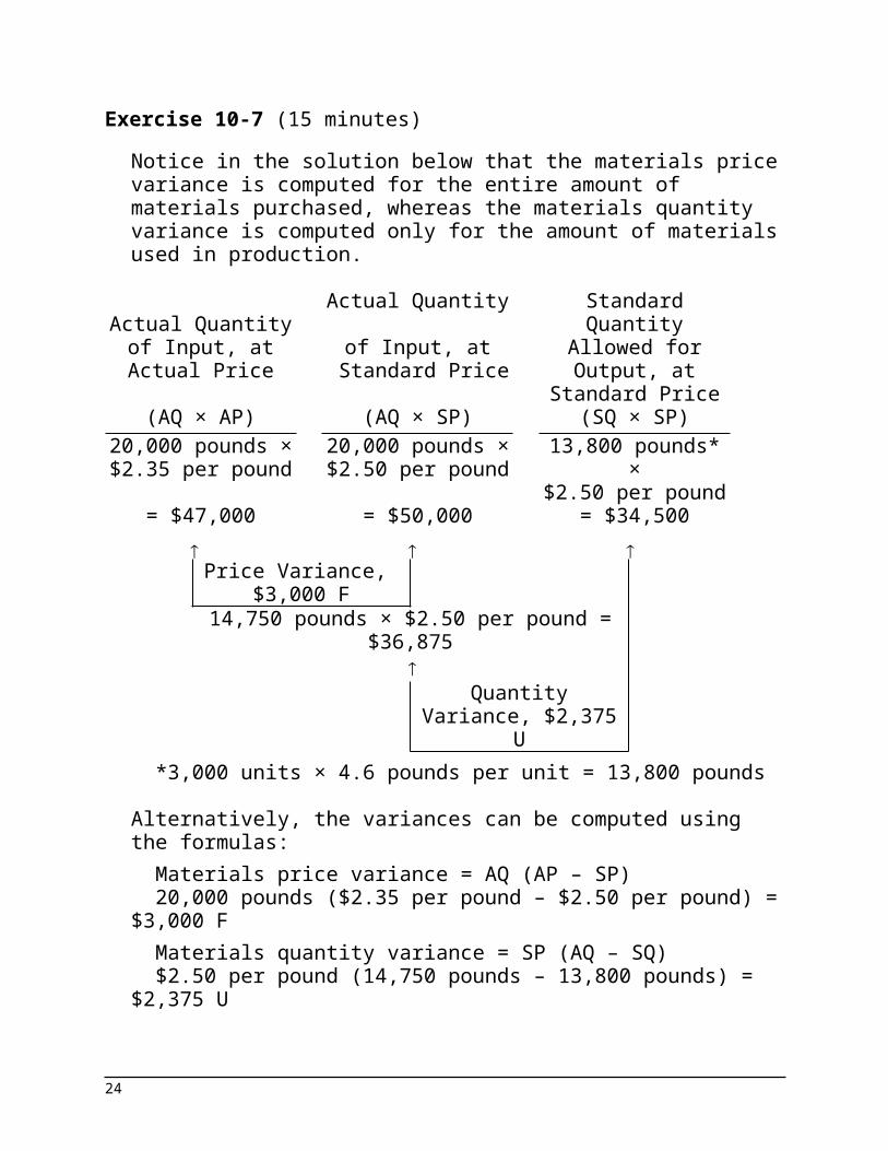
Exercise 10-7 (15 minutes)Notice in the solution below that the materials price variance is computed for the entire amount of materials purchased, whereas the materials quantity variance is computed only for the amount of materials used in production.
Actual Quantity of Input, at Actual
Price
Actual Quantity of Input, at
Standard Price
Standard Quantity Allowed for Output, at
Standard Price(AQ × AP) (AQ × SP) (SQ × SP)
20,000 pounds ×$2.35 per pound
20,000 pounds ×$2.50 per pound
13,800 pounds* ×$2.50 per pound
= $47,000 = $50,000 = $34,500
Price Variance, $3,000 F
14,750 pounds × $2.50 per pound = $36,875
Quantity Variance,
$2,375 U*3,000 units × 4.6 pounds per unit = 13,800 pounds
Alternatively, the variances can be computed using the formulas:
Materials price variance = AQ (AP – SP)20,000 pounds ($2.35 per pound – $2.50 per pound) =
$3,000 FMaterials quantity variance = SP (AQ – SQ)$2.50 per pound (14,750 pounds – 13,800 pounds) = $2,375
U
18
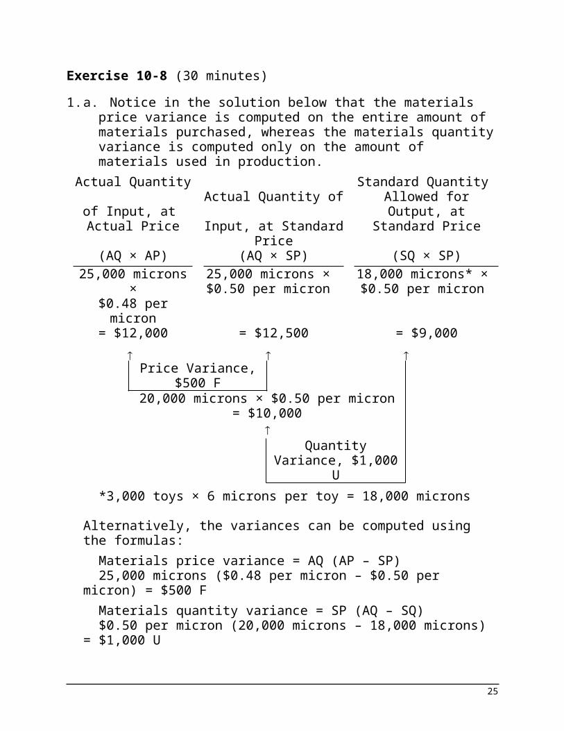
Exercise 10-8 (30 minutes)1. a. Notice in the solution below that the materials price variance
is computed on the entire amount of materials purchased, whereas the materials quantity variance is computed only on the amount of materials used in production.
Actual Quantity of Input, at Actual Price
Actual Quantity of Input, at Standard
Price
Standard Quantity Allowed for Output, at
Standard Price
(AQ × AP) (AQ × SP) (SQ × SP)25,000 microns ×$0.48 per micron
25,000 microns ×$0.50 per micron
18,000 microns* ×$0.50 per micron
= $12,000 = $12,500 = $9,000
Price Variance, $500 F
20,000 microns × $0.50 per micron= $10,000
Quantity Variance,
$1,000 U*3,000 toys × 6 microns per toy = 18,000 microns
Alternatively, the variances can be computed using the formulas:
Materials price variance = AQ (AP – SP)25,000 microns ($0.48 per micron – $0.50 per micron) =
$500 FMaterials quantity variance = SP (AQ – SQ)$0.50 per micron (20,000 microns – 18,000 microns) =
$1,000 U
19
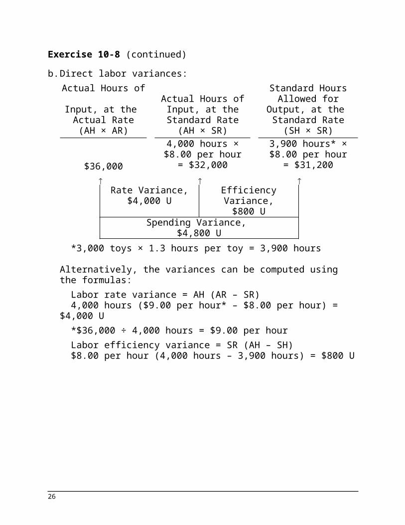
Exercise 10-8 (continued)b. Direct labor variances:
Actual Hours of Input, at the Actual Rate
Actual Hours of Input, at the
Standard Rate
Standard Hours Allowed for Output,
at the Standard Rate
(AH × AR) (AH × SR) (SH × SR)4,000 hours ×$8.00 per hour
3,900 hours* ×$8.00 per hour
$36,000 = $32,000 = $31,200
Rate Variance,$4,000 U
Efficiency Variance,$800 U
Spending Variance, $4,800 U
*3,000 toys × 1.3 hours per toy = 3,900 hours
Alternatively, the variances can be computed using the formulas:
Labor rate variance = AH (AR – SR)4,000 hours ($9.00 per hour* – $8.00 per hour) = $4,000 U*$36,000 ÷ 4,000 hours = $9.00 per hourLabor efficiency variance = SR (AH – SH)$8.00 per hour (4,000 hours – 3,900 hours) = $800 U
20

Exercise 10-8 (continued)2. A variance usually has many possible explanations. In
particular, we should always keep in mind that the standards themselves may be incorrect. Some of the other possible explanations for the variances observed at Dawson Toys appear below:Materials Price Variance Since this variance is favorable, the actual price paid per unit for the material was less than the standard price. This could occur for a variety of reasons including the purchase of a lower grade material at a discount, buying in an unusually large quantity to take advantage of quantity discounts, a change in the market price of the material, or particularly sharp bargaining by the purchasing department.Materials Quantity Variance Since this variance is unfavorable, more materials were used to produce the actual output than were called for by the standard. This could also occur for a variety of reasons. Some of the possibilities include poorly trained or supervised workers, improperly adjusted machines, and defective materials.Labor Rate Variance Since this variance is unfavorable, the actual average wage rate was higher than the standard wage rate. Some of the possible explanations include an increase in wages that has not been reflected in the standards, unanticipated overtime, and a shift toward more highly paid workers.Labor Efficiency Variance Since this variance is unfavorable, the actual number of labor hours was greater than the standard labor hours allowed for the actual output. As with the other variances, this variance could have been caused by any of a number of factors. Some of the possible explanations include poor supervision, poorly trained workers, low-quality materials requiring more labor time to process, and machine breakdowns. In addition, if the direct labor force is essentially fixed, an unfavorable labor efficiency variance could be caused by a reduction in output due to decreased demand for the company’s products.It is worth noting that all of these variances could have been
21
caused by the purchase of low quality materials at a cut-rate price.
22
Problem 10-9 (45 minutes)This problem is more difficult than it looks. Allow ample time for discussion.
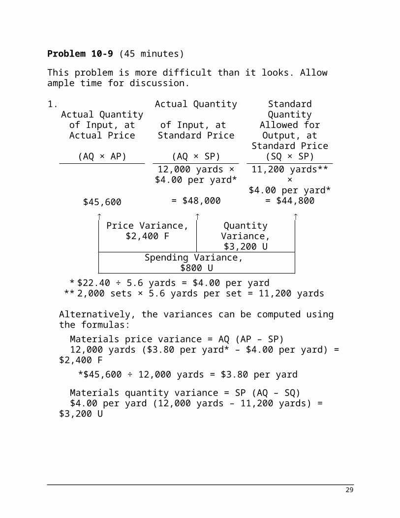
1.Actual Quantity of
Input, at Actual Price
Actual Quantity of Input, at
Standard Price
Standard Quantity Allowed for Output, at
Standard Price(AQ × AP) (AQ × SP) (SQ × SP)
12,000 yards ×$4.00 per yard*
11,200 yards** ×$4.00 per yard*
$45,600 = $48,000 = $44,800
Price Variance,$2,400 F
Quantity Variance,$3,200 U
Spending Variance, $800 U
* $22.40 ÷ 5.6 yards = $4.00 per yard** 2,000 sets × 5.6 yards per set = 11,200 yards
Alternatively, the variances can be computed using the formulas:
Materials price variance = AQ (AP – SP)12,000 yards ($3.80 per yard* – $4.00 per yard) = $2,400 F
*$45,600 ÷ 12,000 yards = $3.80 per yardMaterials quantity variance = SP (AQ – SQ)$4.00 per yard (12,000 yards – 11,200 yards) = $3,200 U
23
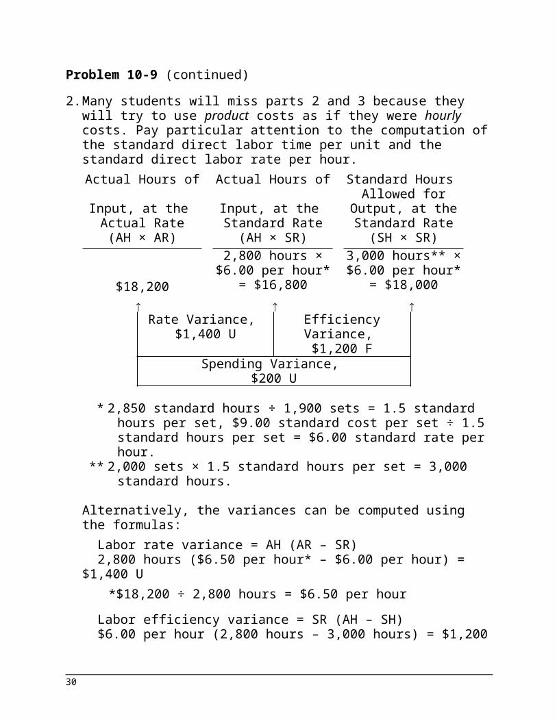
Problem 10-9 (continued)2. Many students will miss parts 2 and 3 because they will try to
use product costs as if they were hourly costs. Pay particular attention to the computation of the standard direct labor time per unit and the standard direct labor rate per hour.
Actual Hours of Input, at the Actual Rate
Actual Hours of Input, at the
Standard Rate
Standard Hours Allowed for
Output, at the Standard Rate
(AH × AR) (AH × SR) (SH × SR)2,800 hours ×
$6.00 per hour*3,000 hours** ×$6.00 per hour*
$18,200 = $16,800 = $18,000
Rate Variance, $1,400 U
Efficiency Variance, $1,200 F
Spending Variance, $200 U
* 2,850 standard hours ÷ 1,900 sets = 1.5 standard hours per set, $9.00 standard cost per set ÷ 1.5 standard hours per set = $6.00 standard rate per hour.
** 2,000 sets × 1.5 standard hours per set = 3,000 standard hours.
Alternatively, the variances can be computed using the formulas:
Labor rate variance = AH (AR – SR)2,800 hours ($6.50 per hour* – $6.00 per hour) = $1,400 U
*$18,200 ÷ 2,800 hours = $6.50 per hourLabor efficiency variance = SR (AH – SH)$6.00 per hour (2,800 hours – 3,000 hours) = $1,200 F
24
Problem 10-9 (continued)3. Actual Hours of
Input, at the Actual Rate
Actual Hours of Input, at the
Standard Rate
Standard Hours Allowed for
Output, at the Standard Rate
(AH × AR) (AH × SR) (SH × SR)2,800 hours ×
$2.40 per hour*3,000 hours ×
$2.40 per hour*$7,000 = $6,720 = $7,200
Rate Variance,
$280 UEfficiency Variance,
$480 FSpending Variance,
$200 F*$3.60 standard cost per set ÷ 1.5 standard hours per set
= $2.40 standard rate per hour
Alternatively, the variances can be computed using the formulas:
Variable overhead rate variance = AH (AR – SR)2,800 hours ($2.50 per hour* – $2.40 per hour) = $280 U
*$7,000 ÷ 2,800 hours = $2.50 per hourVariable overhead efficiency variance = SR (AH – SH)$2.40 per hour (2,800 hours – 3,000 hours) = $480 F
25
Problem 10-10 (45 minutes)
1.Standard Quantity or Hours
Standard Price or Rate
Standard Cost
Alpha6:Direct materials—X442. 1.8 kilos $3.50 per kilo $ 6.30Direct materials—Y661. 2.0 liters $1.40 per liter 2.80Direct labor—Sintering.. 0.20
hours$19.80 per
hour3.96
Direct labor—Finishing. . 0.80 hours
$19.20 per hour
15.36
Total.............................. $28.42Zeta7:Direct materials—X442. 3.0 kilos $3.50 per kilo $10.50Direct materials—Y661. 4.5 liters $1.40 per liter 6.30Direct labor—Sintering.. 0.35
hours$19.80 per
hour6.93
Direct labor—Finishing. . 0.90 hours
$19.20 per hour
17.28
Total.............................. $41.01
26
Problem 10-10 (continued)
2. The computations to follow will require the standard quantities allowed for the actual output for each material.
Standard Quantity AllowedMaterial X442:Production of Alpha6 (1.8 kilos per unit × 1,500 units)........................................................................
2,700 kilos
Production of Zeta7 (3.0 kilos per unit × 2,000 units)........................................................................
6,000 kilos
Total......................................................................... 8,700 kilosMaterial Y661:Production of Alpha6 (2.0 liters per unit × 1,500 units)........................................................................
3,000 liters
Production of Zeta7 (4.5 liters per unit × 2,000 units)........................................................................
9,000 liters
Total......................................................................... 12,000 liters
Direct Materials Variances—Material X442:Materials quantity variance = SP (AQ – SQ)
= $3.50 per kilo (8,500 kilos – 8,700 kilos)= $700 F
Materials price variance = AQ (AP – SP)= 14,500 kilos ($3.60 per kilo* – $3.50 per kilo)= $1,450 U*$52,200 ÷ 14,500 kilos = $3.60 per kilo
Direct Materials Variances—Material Y661:Materials quantity variance = SP (AQ – SQ)
= $1.40 per liter (13,000 liters – 12,000 liters)= $1,400 U
Materials price variance = AQ (AP – SP)= 15,500 liters ($1.35 per liter* – $1.40 per liter)= $775 F*$20,925 ÷ 15,500 liters = $1.35 per liter
27

Problem 10-10 (continued)
3. The computations to follow will require the standard quantities allowed for the actual output for direct labor in each department.
Standard Hours AllowedSintering:Production of Alpha6 (0.20 hours per unit × 1,500 units)........................................................................
300 hours
Production of Zeta7 (0.35 hours per unit × 2,000 units)........................................................................
700 hours
Total......................................................................... 1,000 hours
Finishing:Production of Alpha6 (0.80 hours per unit × 1,500 units)........................................................................
1,200 hours
Production of Zeta7 (0.90 hours per unit × 2,000 units)........................................................................
1,800 hours
Total......................................................................... 3,000 hours
Direct Labor Variances—Sintering:Labor efficiency variance = SR (AH – SH)
= $19.80 per hour (1,200 hours – 1,000 hours)= $3,960 U
Labor rate variance = AH (AR – SR)= 1,200 hours ($22.50 per hour* – $19.80 per hour)= $3,240 U*$27,000 ÷ 1,200 hours = $22.50 per hour
Direct Labor Variances—Finishing:Labor efficiency variance = SR (AH – SH)
= $19.20 per hour (2,850 hours – 3,000 hours)= $2,880 F
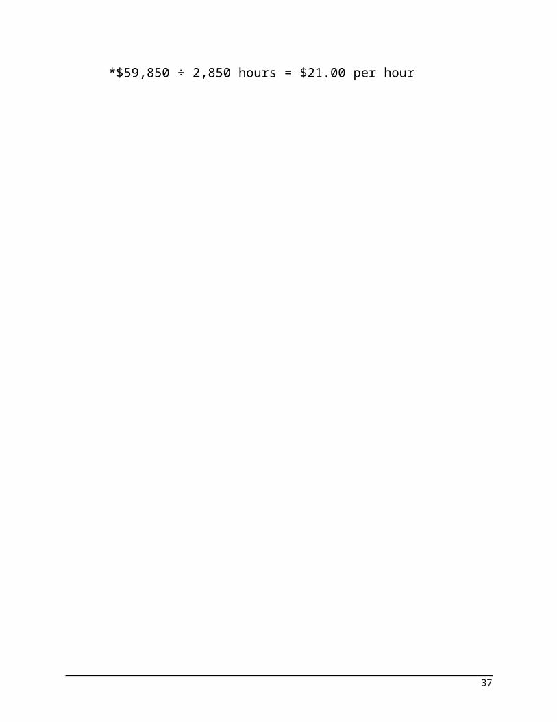
Labor rate variance = AH (AR – SR)= 2,850 hours ($21.00 per hour* – $19.20 per hour)= $5,130 U*$59,850 ÷ 2,850 hours = $21.00 per hour
28
Problem 10-11 (45 minutes)1. a. Materials quantity variance = SP (AQ – SQ)
$5.00 per foot (AQ – 9,600 feet*) = $4,500 U$5.00 per foot × AQ – $48,000 = $4,500**$5.00 per foot × AQ = $52,500AQ = 10,500 feet
* $3,200 units × 3 foot per unit** When used with the formula, unfavorable variances
are positive and favorable variances are negative.
Therefore, $55,650 ÷ 10,500 feet = $5.30 per foot
b. Materials price variance = AQ (AP – SP)10,500 feet ($5.30 per foot – $5.00 per foot) = $3,150 UThe total variance for materials is:
Materials price variance............ $3,150 UMaterials quantity variance....... 4,500 UTotal variance............................ $7,650 U
Alternative approach to parts (a) and (b):
Actual Quantity of Input, at Actual
Price
Actual Quantity of Input, at
Standard Price
Standard Quantity Allowed for Output, at Standard Price
(AQ × AP) (AQ × SP) (SQ × SP)10,500 feet ×$5.30 per foot
10,500 feet ×$5.00 per foot*
9,600 feet** ×$5.00 per foot*
= $55,650* = $52,500 = $48,000
Price Variance, $3,150 U
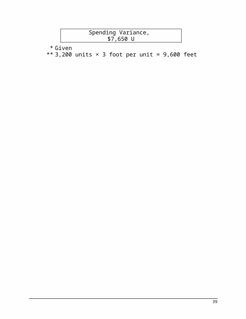
Quantity Variance, $4,500 U*
Spending Variance, $7,650 U
* Given** 3,200 units × 3 foot per unit = 9,600 feet
29
Problem 10-11 (continued)2. a. Labor rate variance = AH (AR – SR)
4,900 hours ($7.50 per hour* – SR) = $2,450 F**$36,750 – 4,900 hours × SR = –$2,450***4,900 hours × SR = $39,200SR = $8.00
* $36,750 ÷ 4,900 hours** $1,650 F + $800 U.
*** When used with the formula, unfavorable variances are positive and favorable variances are negative.
b. Labor efficiency variance = SR (AH – SH) $8 per hour (4,900 hours – SH) = $800 U$39,200 – $8 per hour × SH = $800*$8 per hour × SH = $38,400SH = 4,800 hours* When used with the formula, unfavorable variances are
positive and favorable variances are negative.
Alternative approach to parts (a) and (b):Actual Hours of
Input, at the Actual Rate
Actual Hours of Input, at the
Standard Rate
Standard Hours Allowed for Output,
at the Standard Rate
(AH × AR) (AH × SR) (SH × SR)4,900 hours* ×$8.00 per hour
4,800 hours ×$8.00 per hour
$36,750* = $39,200 = $38,400
Rate Variance,$2,450 F
Efficiency Variance,$800 U*
Spending Variance, $1,650 F*
*Given.
c. The standard hours allowed per unit of product are:
30
4,800 hours ÷ 3,200 units = 1.5 hours per unitProblem 10-12 (45 minutes)1. The standard quantity of plates allowed for tests performed
during the month would be:Blood tests............................... 1,800Smears.................................... 2,400Total......................................... 4,200Plates per test......................... × 2 Standard quantity allowed....... 8,400
The variance analysis for plates would be:
Actual Quantity of Input, at Actual
Price
Actual Quantity of Input, at
Standard Price
Standard Quantity Allowed for Output, at
Standard Price(AQ × AP) (AQ × SP) (SQ × SP)
12,000 plates ×$2.50 per plate
8,400 plates ×$2.50 per plate
$28,200 = $30,000 = $21,000
Price Variance,$1,800 F
10,500 plates × $2.50 per plate
= $26,250
Quantity Variance, $5,250 U
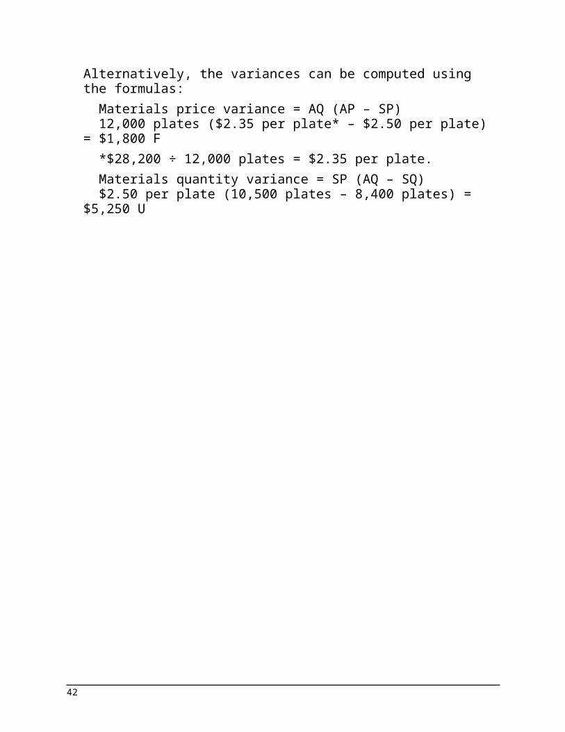
Alternatively, the variances can be computed using the formulas:
Materials price variance = AQ (AP – SP)12,000 plates ($2.35 per plate* – $2.50 per plate) = $1,800 F*$28,200 ÷ 12,000 plates = $2.35 per plate.Materials quantity variance = SP (AQ – SQ)$2.50 per plate (10,500 plates – 8,400 plates) = $5,250 U
31
Problem 10-12 (continued)2. a. The standard hours allowed for tests performed during the
month would be:Blood tests: 0.3 hour per test × 1,800 tests. . 540 hoursSmears: 0.15 hour per test × 2,400 tests...... 360 hoursTotal standard hours allowed......................... 900 hours
The variance analysis would be:Actual Hours of
Input, at the Actual Rate
Actual Hours of Input, at the
Standard Rate
Standard Hours Allowed for Output,
at the Standard Rate
(AH × AR) (AH × SR) (SH × SR)1,150 hours ×
$14.00 per hour900 hours ×
$14.00 per hour$13,800 = $16,100 = $12,600
Rate Variance,
$2,300 FEfficiency Variance,
$3,500 USpending Variance,
$1,200 U
Alternatively, the variances can be computed using the formulas:
Labor rate variance = AH (AR – SR)1,150 hours ($12.00 per hour* – $14.00 per hour) = $2,300 F*$13,800 ÷ 1,150 hours = $12.00 per hourLabor efficiency variance = SR (AH – SH) $14.00 per hour (1,150 hours – 900 hours) = $3,500 U
32

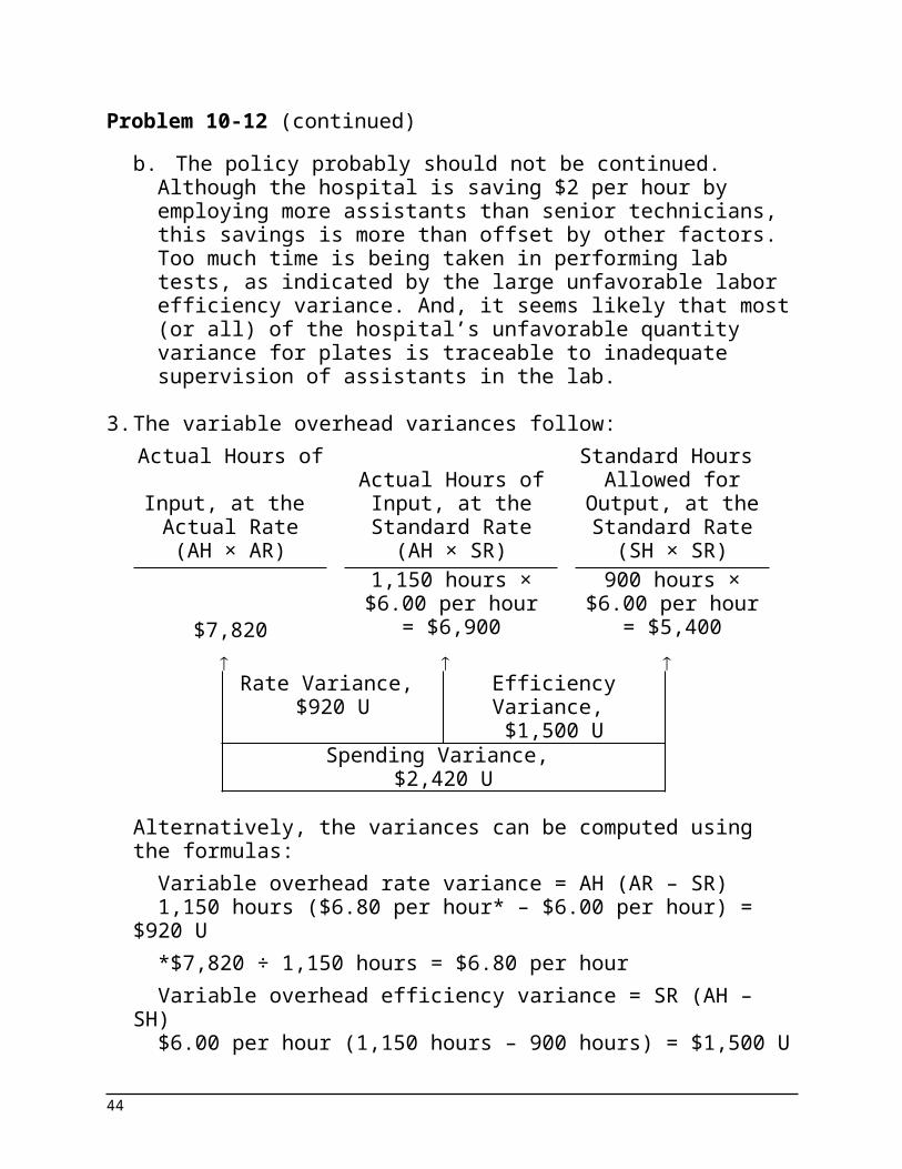
Problem 10-12 (continued)b. The policy probably should not be continued. Although the
hospital is saving $2 per hour by employing more assistants than senior technicians, this savings is more than offset by other factors. Too much time is being taken in performing lab tests, as indicated by the large unfavorable labor efficiency variance. And, it seems likely that most (or all) of the hospital’s unfavorable quantity variance for plates is traceable to inadequate supervision of assistants in the lab.
3. The variable overhead variances follow:Actual Hours of
Input, at the Actual Rate
Actual Hours of Input, at the
Standard Rate
Standard Hours Allowed for
Output, at the Standard Rate
(AH × AR) (AH × SR) (SH × SR)1,150 hours ×$6.00 per hour
900 hours ×$6.00 per hour
$7,820 = $6,900 = $5,400
Rate Variance, $920 U
Efficiency Variance, $1,500 U
Spending Variance, $2,420 U
Alternatively, the variances can be computed using the formulas:
Variable overhead rate variance = AH (AR – SR)1,150 hours ($6.80 per hour* – $6.00 per hour) = $920 U*$7,820 ÷ 1,150 hours = $6.80 per hourVariable overhead efficiency variance = SR (AH – SH)$6.00 per hour (1,150 hours – 900 hours) = $1,500 U
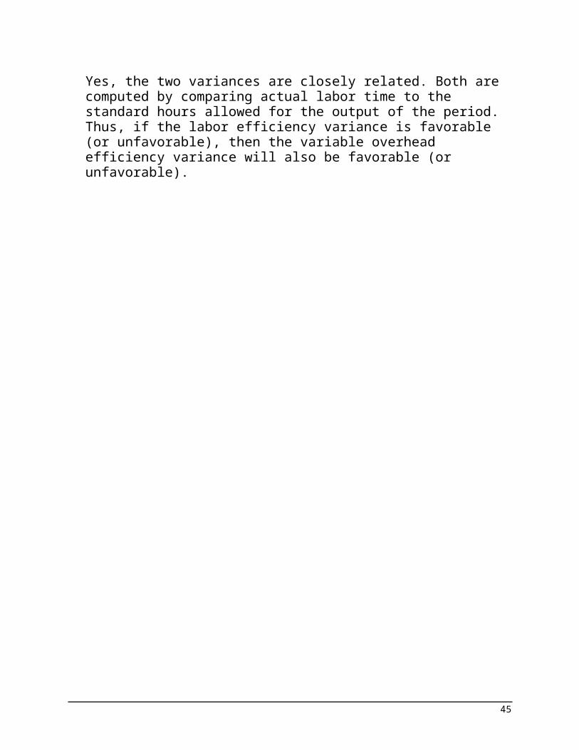
Yes, the two variances are closely related. Both are computed by comparing actual labor time to the standard hours allowed for the output of the period. Thus, if the labor efficiency variance is favorable (or unfavorable), then the variable overhead efficiency variance will also be favorable (or
33
unfavorable).
34
Problem 10-13 (45 minutes)
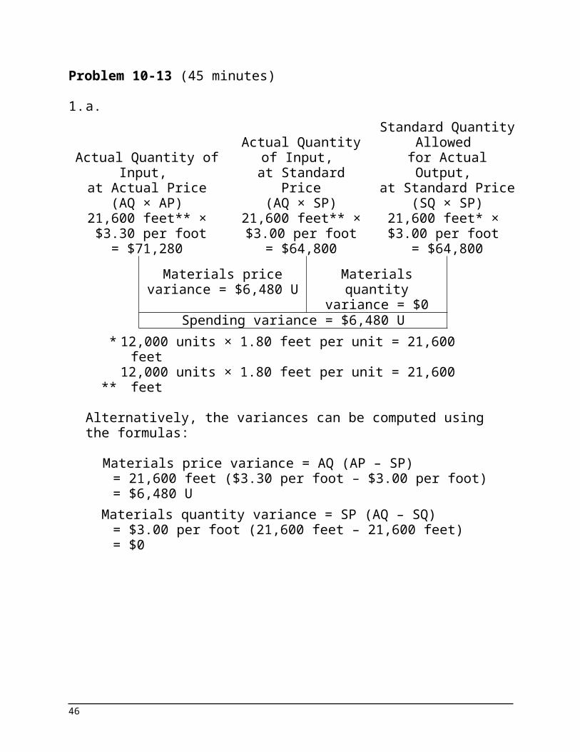
1. a.
Actual Quantity of Input,
at Actual Price(AQ × AP)
Actual Quantity of Input,
at Standard Price(AQ × SP)
Standard Quantity Allowed
for Actual Output, at Standard Price
(SQ × SP)21,600 feet** × $3.30 per foot
= $71,280
21,600 feet** ×$3.00 per foot
= $64,800
21,600 feet* × $3.00 per foot
= $64,800Materials price
variance = $6,480 UMaterials quantity
variance = $0Spending variance = $6,480 U
* 12,000 units × 1.80 feet per unit = 21,600 feet** 12,000 units × 1.80 feet per unit = 21,600 feet
Alternatively, the variances can be computed using the formulas:
Materials price variance = AQ (AP – SP)= 21,600 feet ($3.30 per foot – $3.00 per foot) = $6,480 U
Materials quantity variance = SP (AQ – SQ)= $3.00 per foot (21,600 feet – 21,600 feet)= $0
35

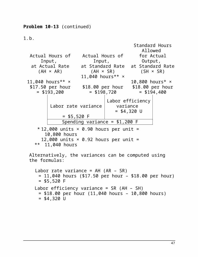
Problem 10-13 (continued)
1. b.
Actual Hours of Input, at Actual Rate
(AH × AR)
Actual Hours of Input,
at Standard Rate(AH × SR)
Standard Hours Allowed
for Actual Output, at Standard Rate
(SH × SR)11,040 hours** × $17.50 per hour
= $193,200
11,040 hours** × $18.00 per hour
= $198,720
10,800 hours* × $18.00 per hour
= $194,400
Labor rate variance = $5,520 F
Labor efficiency variance
= $4,320 USpending variance = $1,200 F
* 12,000 units × 0.90 hours per unit = 10,800 hours
**12,000 units × 0.92 hours per unit = 11,040
hours
Alternatively, the variances can be computed using the formulas:
Labor rate variance = AH (AR – SR)= 11,040 hours ($17.50 per hour – $18.00 per hour)= $5,520 F
Labor efficiency variance = SR (AH – SH)= $18.00 per hour (11,040 hours – 10,800 hours)= $4,320 U
36
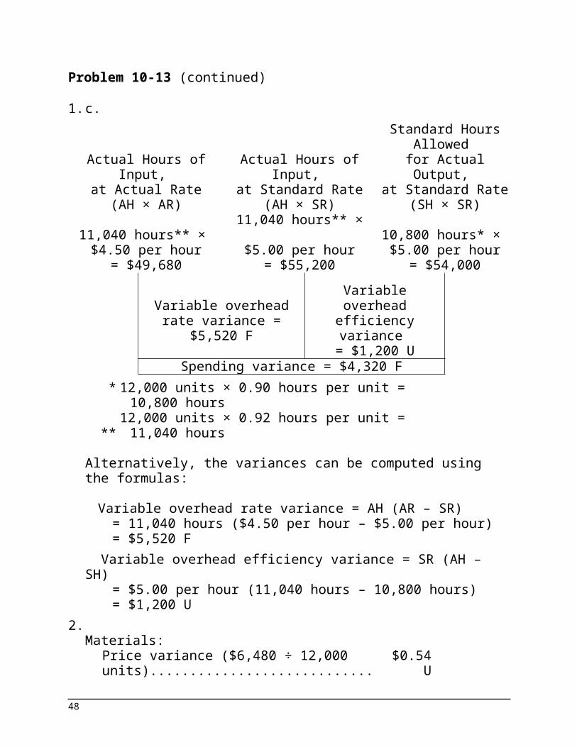
Problem 10-13 (continued)
1. c.
Actual Hours of Input, at Actual Rate
(AH × AR)
Actual Hours of Input,
at Standard Rate(AH × SR)
Standard Hours Allowed
for Actual Output, at Standard Rate
(SH × SR)11,040 hours** ×
$4.50 per hour= $49,680
11,040 hours** × $5.00 per hour
= $55,200
10,800 hours* × $5.00 per hour
= $54,000
Variable overhead rate variance = $5,520 F
Variable overhead efficiency variance
= $1,200 USpending variance = $4,320 F
* 12,000 units × 0.90 hours per unit = 10,800 hours
**12,000 units × 0.92 hours per unit = 11,040
hours
Alternatively, the variances can be computed using the formulas:
Variable overhead rate variance = AH (AR – SR)= 11,040 hours ($4.50 per hour – $5.00 per hour)= $5,520 F
Variable overhead efficiency variance = SR (AH – SH)= $5.00 per hour (11,040 hours – 10,800 hours)= $1,200 U
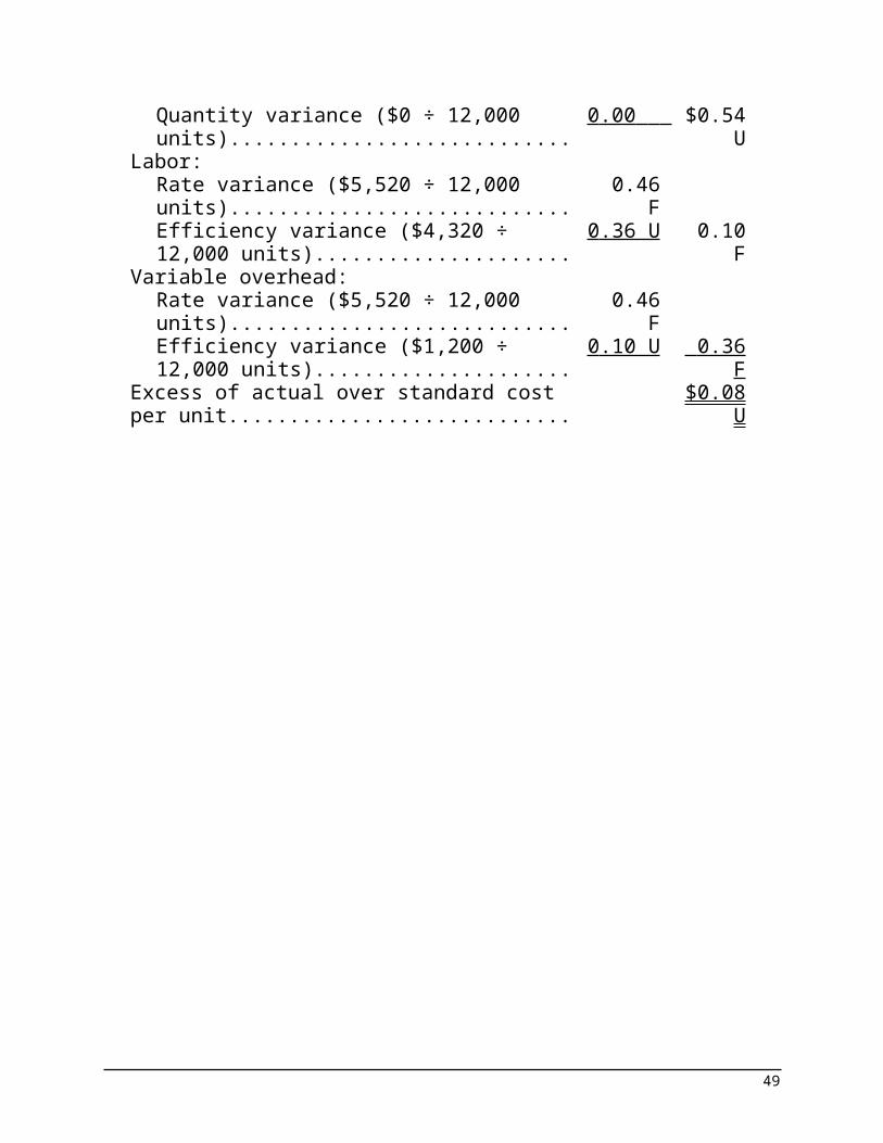
2.Materials:
Price variance ($6,480 ÷ 12,000 units)... $0.54 U
Quantity variance ($0 ÷ 12,000 units).... 0 .00 $0.54 U
Labor:Rate variance ($5,520 ÷ 12,000 units).... 0.46 FEfficiency variance ($4,320 ÷ 12,000 0 .36 U 0.10 F
37

units).......................................................Variable overhead:
Rate variance ($5,520 ÷ 12,000 units).... 0.46 FEfficiency variance ($1,200 ÷ 12,000 units).......................................................
0 .10 U 0.36 F
Excess of actual over standard cost per unit..............................................................
$0.08 U
38
Problem 10-13 (continued)
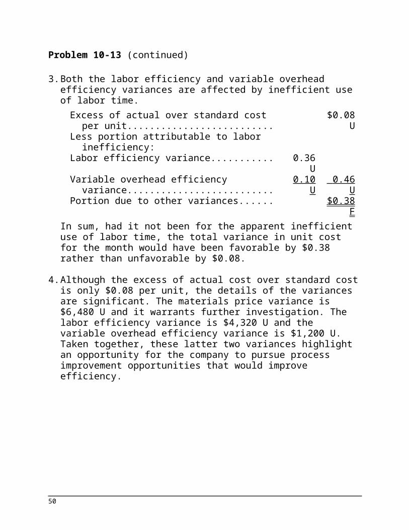
3. Both the labor efficiency and variable overhead efficiency variances are affected by inefficient use of labor time.
Excess of actual over standard cost per unit $0.08 U
Less portion attributable to labor inefficiency:
Labor efficiency variance............................. 0.36 UVariable overhead efficiency variance......... 0.10 U 0.46
UPortion due to other variances.................... $0.38
FIn sum, had it not been for the apparent inefficient use of labor time, the total variance in unit cost for the month would have been favorable by $0.38 rather than unfavorable by $0.08.
4. Although the excess of actual cost over standard cost is only $0.08 per unit, the details of the variances are significant. The materials price variance is $6,480 U and it warrants further investigation. The labor efficiency variance is $4,320 U and the variable overhead efficiency variance is $1,200 U. Taken together, these latter two variances highlight an opportunity for the company to pursue process improvement opportunities that would improve efficiency.
39

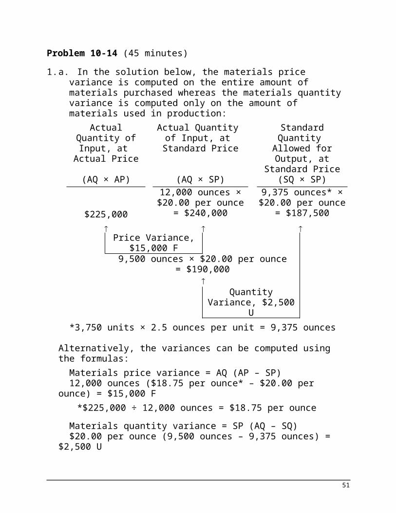
Problem 10-14 (45 minutes)1. a. In the solution below, the materials price variance is
computed on the entire amount of materials purchased whereas the materials quantity variance is computed only on the amount of materials used in production:Actual Quantity
of Input, at Actual Price
Actual Quantity of Input, at
Standard Price
Standard Quantity Allowed for Output, at Standard Price
(AQ × AP) (AQ × SP) (SQ × SP)12,000 ounces ×$20.00 per ounce
9,375 ounces* ×$20.00 per ounce
$225,000 = $240,000 = $187,500
Price Variance,$15,000 F
9,500 ounces × $20.00 per ounce= $190,000
Quantity Variance,
$2,500 U*3,750 units × 2.5 ounces per unit = 9,375 ounces
Alternatively, the variances can be computed using the formulas:
Materials price variance = AQ (AP – SP)12,000 ounces ($18.75 per ounce* – $20.00 per ounce) =
$15,000 F*$225,000 ÷ 12,000 ounces = $18.75 per ounce
Materials quantity variance = SP (AQ – SQ)$20.00 per ounce (9,500 ounces – 9,375 ounces) = $2,500 U
b. Yes, the contract probably should be signed. The new price of $18.75 per ounce is substantially lower than the old price of $20.00 per ounce, resulting in a favorable price variance of $15,000 for the month. Moreover, the material from the new supplier appears to cause little or no problem in production as shown by the small materials quantity variance for the
40

month.
41
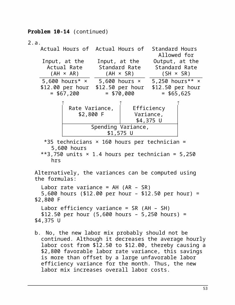
Problem 10-14 (continued)2. a.
Actual Hours of Input, at the Actual Rate
Actual Hours of Input, at the
Standard Rate
Standard Hours Allowed for Output,
at the Standard Rate
(AH × AR) (AH × SR) (SH × SR)5,600 hours* ×$12.00 per hour
5,600 hours ×$12.50 per hour
5,250 hours** ×$12.50 per hour
= $67,200 = $70,000 = $65,625
Rate Variance,$2,800 F
Efficiency Variance,$4,375 U
Spending Variance,$1,575 U
*35 technicians × 160 hours per technician = 5,600 hours
**3,750 units × 1.4 hours per technician = 5,250 hrs
Alternatively, the variances can be computed using the formulas:
Labor rate variance = AH (AR – SR)5,600 hours ($12.00 per hour – $12.50 per hour) = $2,800 FLabor efficiency variance = SR (AH – SH)$12.50 per hour (5,600 hours – 5,250 hours) = $4,375 U
b. No, the new labor mix probably should not be continued. Although it decreases the average hourly labor cost from $12.50 to $12.00, thereby causing a $2,800 favorable labor rate variance, this savings is more than offset by a large unfavorable labor efficiency variance for the month. Thus, the new labor mix increases overall labor costs.
42

Problem 10-14 (continued)3. Actual Hours of
Input, at the Actual Rate
Actual Hours of Input, at the
Standard Rate
Standard Hours Allowed for
Output, at the Standard Rate
(AH × AR) (AH × SR) (SH × SR)5,600 hours* ×$3.50 per hour
5,250 hours** ×$3.50 per hour
$18,200 = $19,600 = $18,375
Rate Variance,$1,400 F
Efficiency Variance,$1,225 U
Spending Variance,$175 F
* Based on direct labor hours: 35 technicians × 160 hours per technician = 5,600
hours** 3,750 units × 1.4 hours per unit = 5,250 hours
Alternatively, the variances can be computed using the formulas:
Variable overhead rate variance = AH (AR – SR)5,600 hours ($3.25 per hour* – $3.50 per hour) = $1,400 F*$18,200 ÷ 5,600 hours = $3.25 per hourVariable overhead efficiency variance = SR (AH – SH)$3.50 per hour (5,600 hours – 5,250 hours) = $1,225 U
Both the labor efficiency variance and the variable overhead efficiency variance are computed by comparing actual labor-hours to standard labor-hours. Thus, if the labor efficiency variance is unfavorable, then the variable overhead efficiency variance will be unfavorable as well.
43
Problem 10-15 (45 minutes)1. a.
Actual Quantity of Input, at Actual
Price
Actual Quantity of Input, at
Standard Price
Standard Quantity Allowed for Output, at
Standard Price(AQ × AP) (AQ × SP) (SQ × SP)
60,000 pounds ×$1.95 per pound
60,000 pounds ×$2.00 per pound
45,000 pounds* ×$2.00 per pound
= $117,000 = $120,000 = $90,000
Price Variance,$3,000 F
49,200 pounds × $2.00 per pound = $98,400
Quantity Variance,
$8,400 U*15,000 pools × 3.0 pounds per pool = 45,000 pounds
Alternatively, the variances can be computed using the formulas:
Materials price variance = AQ (AP – SP)60,000 pounds ($1.95 per pound – $2.00 per pound) =
$3,000 FMaterials quantity variance = SP (AQ – SQ)$2.00 per pound (49,200 pounds – 45,000 pounds) = $8,400
U
44
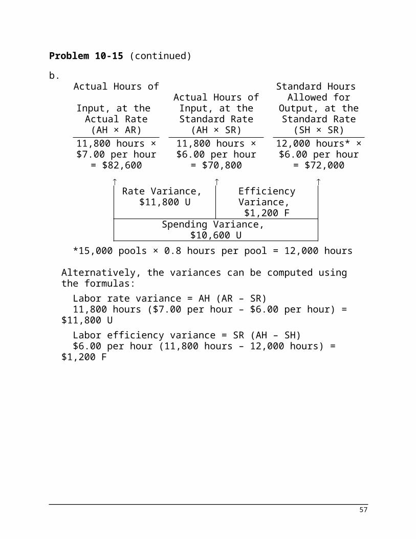
Problem 10-15 (continued)b.
Actual Hours of Input, at the Actual Rate
Actual Hours of Input, at the
Standard Rate
Standard Hours Allowed for
Output, at the Standard Rate
(AH × AR) (AH × SR) (SH × SR)11,800 hours ×$7.00 per hour
11,800 hours ×$6.00 per hour
12,000 hours* ×$6.00 per hour
= $82,600 = $70,800 = $72,000
Rate Variance, $11,800 U
Efficiency Variance, $1,200 F
Spending Variance, $10,600 U
*15,000 pools × 0.8 hours per pool = 12,000 hours
Alternatively, the variances can be computed using the formulas:
Labor rate variance = AH (AR – SR)11,800 hours ($7.00 per hour – $6.00 per hour) = $11,800 ULabor efficiency variance = SR (AH – SH)$6.00 per hour (11,800 hours – 12,000 hours) = $1,200 F
45
Problem 10-15 (continued)c.
Actual Hours of Input, at the Actual Rate
Actual Hours of Input, at the
Standard Rate
Standard Hours Allowed for
Output, at the Standard Rate
(AH × AR) (AH × SR) (SH × SR)5,900 hours ×$3.00 per hour
6,000 hours* ×$3.00 per hour
$18,290 = $17,700 = $18,000
Rate Variance,$590 U
Efficiency Variance,$300 F
Spending Variance, $290 U
*15,000 pools × 0.4 hours per pool = 6,000 hours
Alternatively, the variances can be computed using the formulas:
Variable overhead rate variance = AH (AR – SR)5,900 hours ($3.10 per hour* – $3.00 per hour) = $590 U*$18,290 ÷ 5,900 hours = $3.10 per hourVariable overhead efficiency variance = SR (AH – SH)$3.00 per hour (5,900 hours – 6,000 hours) = $300 F
46
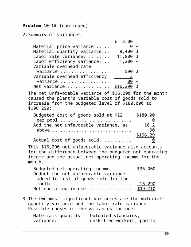
Problem 10-15 (continued)2. Summary of variances:
Material price variance.................... $ 3,000 FMaterial quantity variance............... 8,400 ULabor rate variance......................... 11,800 ULabor efficiency variance................. 1,200 FVariable overhead rate variance...... 590 UVariable overhead efficiency
variance........................................ 300 FNet variance.................................... $16,290 U
The net unfavorable variance of $16,290 for the month caused the plant’s variable cost of goods sold to increase from the budgeted level of $180,000 to $196,290:
Budgeted cost of goods sold at $12 per pool.$180,00
0Add the net unfavorable variance, as above. 16,290
Actual cost of goods sold...............................$196,29
0This $16,290 net unfavorable variance also accounts for the difference between the budgeted net operating income and the actual net operating income for the month.
Budgeted net operating income.................... $36,000Deduct the net unfavorable variance added
to cost of goods sold for the month............. 16,290 Net operating income.................................... $ 19 ,710
3. The two most significant variances are the materials quantity variance and the labor rate variance. Possible causes of the variances include:
Materials quantity variance:
Outdated standards, unskilled workers, poorly adjusted machines, carelessness, poorly trained workers, inferior quality materials.
Labor rate variance: Outdated standards, change in pay scale, overtime pay.
47
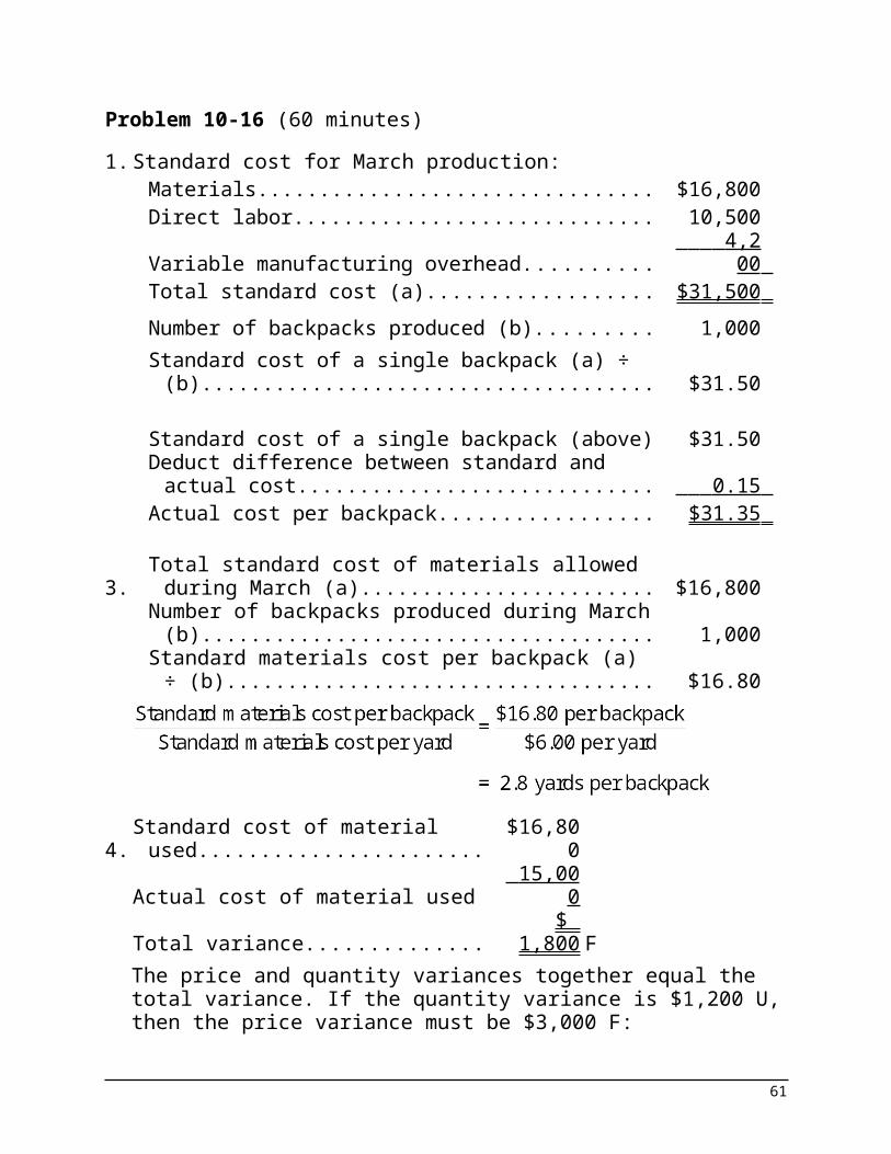
Problem 10-16 (60 minutes)1. Standard cost for March production:
Materials................................................................ $16,800Direct labor............................................................ 10,500Variable manufacturing overhead.......................... 4,200 Total standard cost (a)........................................... $31,500 Number of backpacks produced (b)....................... 1,000Standard cost of a single backpack (a) ÷ (b)......... $31.50
Standard cost of a single backpack (above)........... $31.50Deduct difference between standard and actual
cost..................................................................... 0.15 Actual cost per backpack....................................... $31.35
3.Total standard cost of materials allowed during
March (a)............................................................ $16,800Number of backpacks produced during March (b) 1,000Standard materials cost per backpack (a) ÷ (b). . . $16.80
4. Standard cost of material used.....$16,80
0Actual cost of material used.......... 15,000
Total variance................................$
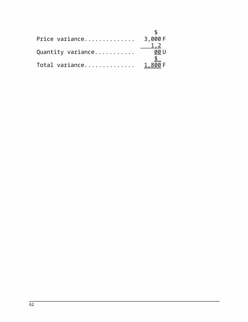
1,800 FThe price and quantity variances together equal the total variance. If the quantity variance is $1,200 U, then the price variance must be $3,000 F:
Price variance................................$
3,000 FQuantity variance.......................... 1,200 U
Total variance................................$
1,800 F
48
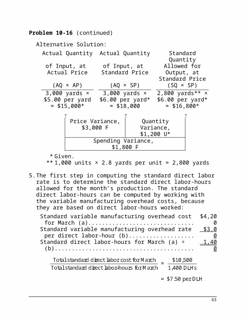
Problem 10-16 (continued)Alternative Solution:
Actual Quantity of Input, at Actual Price
Actual Quantity of Input, at
Standard Price
Standard Quantity Allowed for Output, at
Standard Price(AQ × AP) (AQ × SP) (SQ × SP)
3,000 yards ×$5.00 per yard
3,000 yards ×$6.00 per yard*
2,800 yards** ×$6.00 per yard*
= $15,000* = $18,000 = $16,800*
Price Variance,$3,000 F
Quantity Variance,$1,200 U*
Spending Variance, $1,800 F
* Given.** 1,000 units × 2.8 yards per unit = 2,800 yards
5. The first step in computing the standard direct labor rate is to determine the standard direct labor-hours allowed for the month’s production. The standard direct labor-hours can be computed by working with the variable manufacturing overhead costs, because they are based on direct labor-hours worked:
Standard variable manufacturing overhead cost for March (a).....................................................................
$4,200
Standard variable manufacturing overhead rate per direct labor-hour (b).................................................... $3.00
Standard direct labor-hours for March (a) ÷ (b)............. 1,400
49
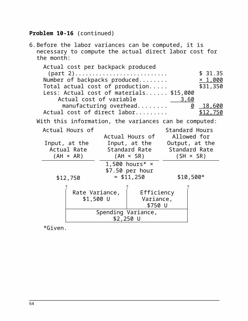
Problem 10-16 (continued)6. Before the labor variances can be computed, it is necessary to
compute the actual direct labor cost for the month:Actual cost per backpack produced (part
2)............................................................... $ 31.35Number of backpacks produced.................. × 1,000Total actual cost of production..................... $31,350Less: Actual cost of materials...................... $15,000
Actual cost of variable manufacturing overhead........................................... 3,600 18,600
Actual cost of direct labor............................ $12,750With this information, the variances can be computed:
Actual Hours of Input, at the Actual Rate
Actual Hours of Input, at the
Standard Rate
Standard Hours Allowed for Output,
at the Standard Rate
(AH × AR) (AH × SR) (SH × SR)1,500 hours* ×$7.50 per hour
$12,750 = $11,250 $10,500*
Rate Variance,$1,500 U
Efficiency Variance,$750 U
Spending Variance,$2,250 U
*Given.
50
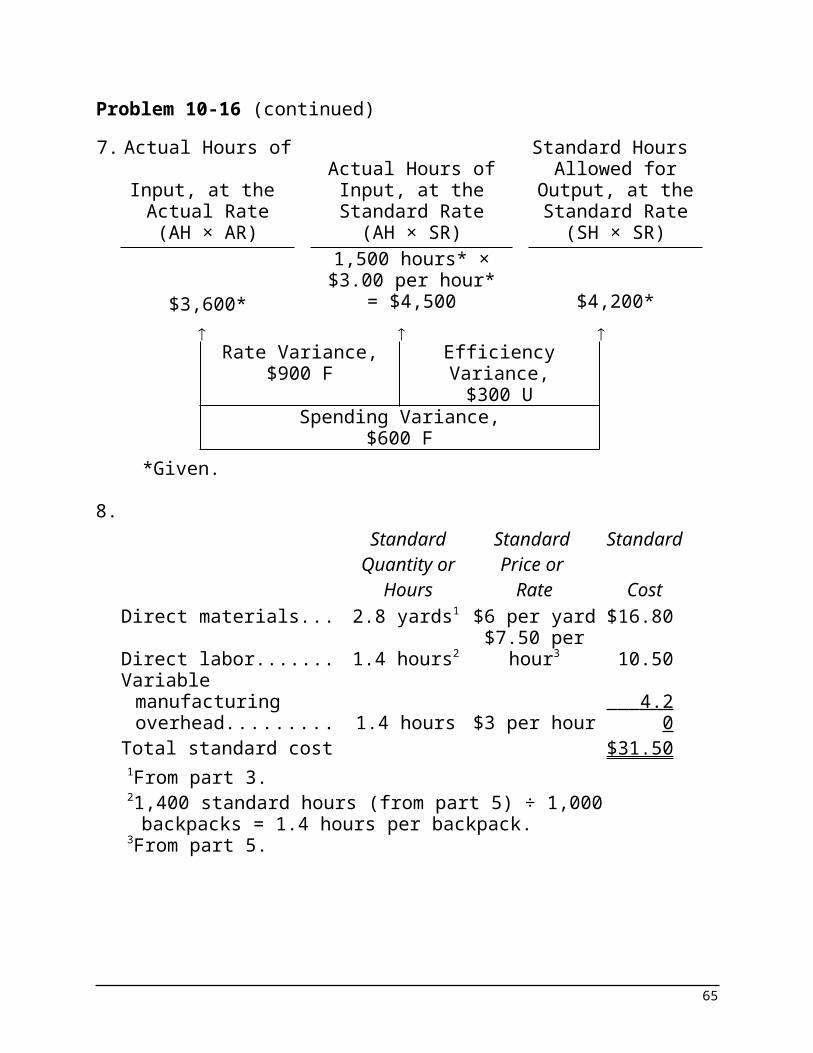
Problem 10-16 (continued)7. Actual Hours of
Input, at the Actual Rate
Actual Hours of Input, at the
Standard Rate
Standard Hours Allowed for
Output, at the Standard Rate
(AH × AR) (AH × SR) (SH × SR)1,500 hours* ×$3.00 per hour*
$3,600* = $4,500 $4,200*
Rate Variance,$900 F
Efficiency Variance,$300 U
Spending Variance,$600 F
*Given.
8.Standard
Quantity or Hours
Standard Price or
Rate
Standard
CostDirect materials.......... 2.8 yards1 $6 per yard $16.80
Direct labor................. 1.4 hours2$7.50 per
hour3 10.50Variable
manufacturing overhead.................. 1.4 hours $3 per hour 4.20
Total standard cost...... $31.501From part 3.21,400 standard hours (from part 5) ÷ 1,000 backpacks
= 1.4 hours per backpack.3From part 5.
51

Case 10-17 (60 minutes)1. The number of units produced can be computed by using the
total standard cost applied for the period for any input—direct materials, direct labor, or variable manufacturing overhead. Using the standard cost applied for direct materials, we have:
The same answer can be obtained by using direct labor or variable manufacturing overhead.
2. 138,000 pounds; see below for a detailed analysis.
3. $2.95 per pound; see below for a detailed analysis.
4. 19,400 direct labor-hours; see below for a detailed analysis.
5. $15.75 per direct labor-hour; see below for a detailed analysis.
6. Standard variable overhead cost applied.......................................... $54,000
Add: Overhead efficiency variance.. 4,200 U (see below)Deduct: Overhead rate variance..... 1,300 FActual variable overhead cost
incurred........................................ $56,900
52
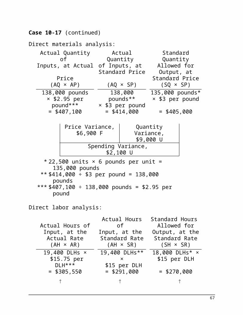
Case 10-17 (continued)Direct materials analysis:
Actual Quantity of Inputs, at Actual
Price
Actual Quantity of Inputs, at
Standard Price
Standard Quantity Allowed for Output, at
Standard Price(AQ × AP) (AQ × SP) (SQ × SP)
138,000 pounds × $2.95 per
pound***
138,000 pounds**
× $3 per pound
135,000 pounds* × $3 per pound
= $407,100 = $414,000 = $405,000
Price Variance, $6,900 F
Quantity Variance,$9,000 U
Spending Variance, $2,100 U
* 22,500 units × 6 pounds per unit = 135,000 pounds
** $414,000 ÷ $3 per pound = 138,000 pounds*** $407,100 ÷ 138,000 pounds = $2.95 per
pound
Direct labor analysis:
Actual Hours of Input, at the Actual
Rate
Actual Hours of Input, at the
Standard Rate
Standard Hours Allowed for
Output, at the Standard Rate
(AH × AR) (AH × SR) (SH × SR)19,400 DLHs ×
$15.75 per DLH***19,400 DLHs** ×
$15 per DLH18,000 DLHs* ×
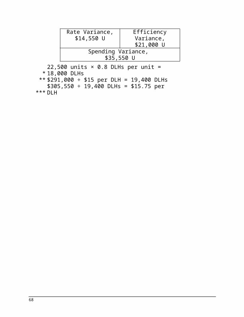
$15 per DLH= $305,550 = $291,000 = $270,000
Rate Variance,
$14,550 UEfficiency Variance,
$21,000 USpending Variance,
$35,550 U* 22,500 units × 0.8 DLHs per unit = 18,000
53
DLHs** $291,000 ÷ $15 per DLH = 19,400 DLHs
*** $305,550 ÷ 19,400 DLHs = $15.75 per DLH
54
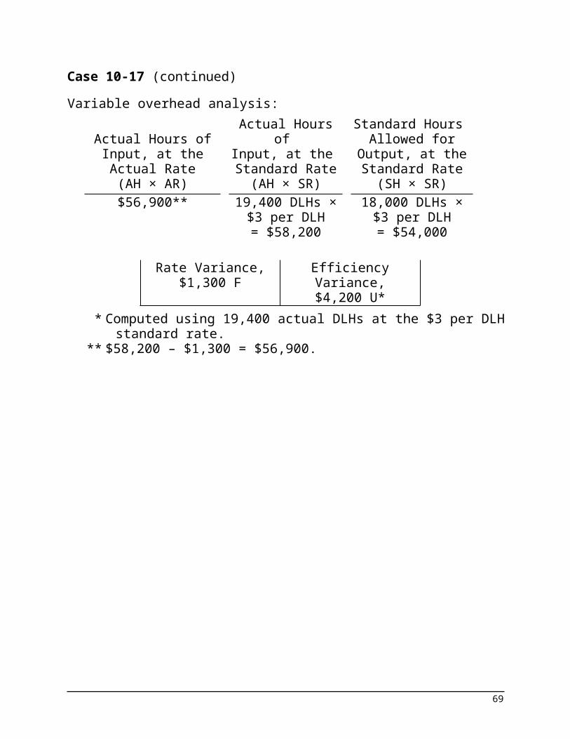
Case 10-17 (continued)Variable overhead analysis:
Actual Hours of Input, at the Actual
Rate
Actual Hours of Input, at the
Standard Rate
Standard Hours Allowed for
Output, at the Standard Rate
(AH × AR) (AH × SR) (SH × SR)$56,900** 19,400 DLHs ×
$3 per DLH18,000 DLHs ×
$3 per DLH= $58,200 = $54,000
Rate Variance,$1,300 F
Efficiency Variance,$4,200 U*
* Computed using 19,400 actual DLHs at the $3 per DLH standard rate.
** $58,200 – $1,300 = $56,900.
55

Appendix 10APredetermined Overhead Rates and Overhead Analysis in a Standard Costing System
Exercise 10A-1 (15 minutes)
1.
2.
56
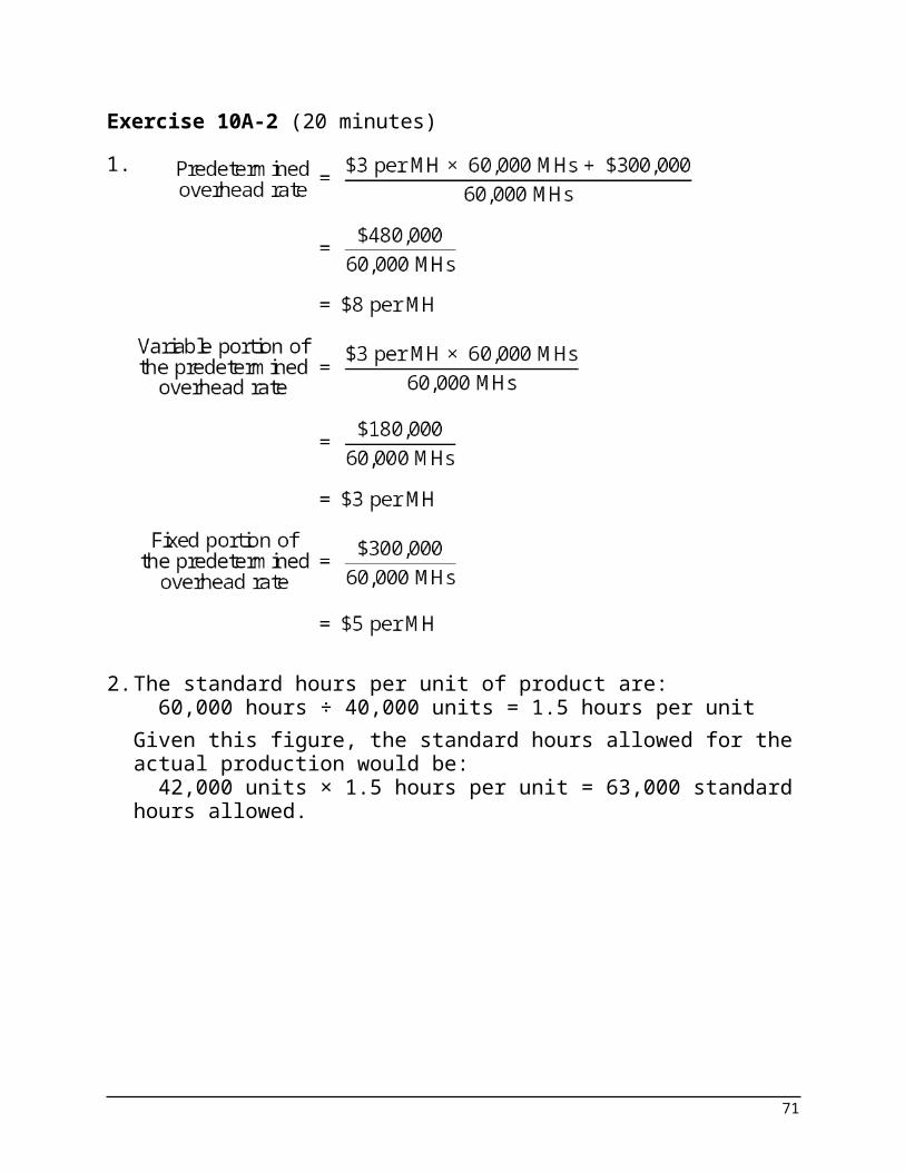
Exercise 10A-2 (20 minutes)1.
2. The standard hours per unit of product are:60,000 hours ÷ 40,000 units = 1.5 hours per unit
Given this figure, the standard hours allowed for the actual production would be:
42,000 units × 1.5 hours per unit = 63,000 standard hours allowed.
57
Exercise 10A-2 (continued)3. Variable overhead rate variance:
Variable overhead rate variance = (AH × AR) – (AH × SR)($185,600) – (64,000 hours × $3 per hour) = $6,400 F
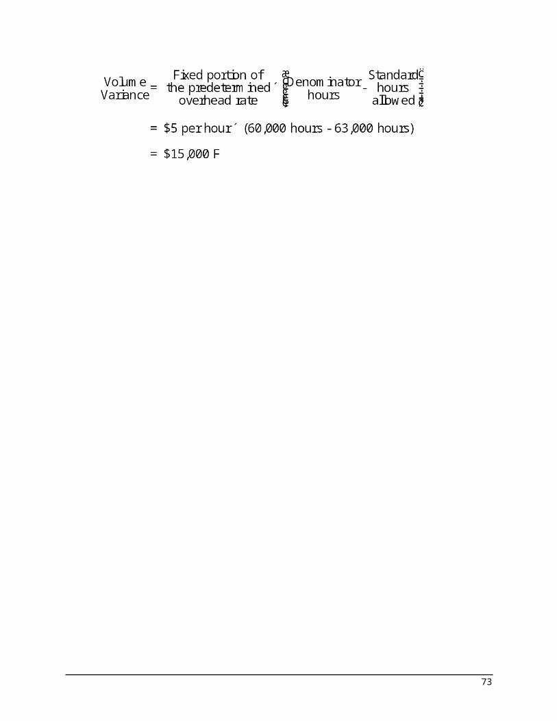
Variable overhead efficiency variance:Variable overhead efficiency variance = SR (AH – SH) $3 per hour (64,000 hours – 63,000 hours) = $3,000 U
The fixed overhead variances are as follows:Actual Fixed Overhead
Budgeted Fixed Overhead
Fixed Overhead Applied to Work in Process
$302,400 $300,000*63,000 hours × $5 per
hour= $315,000
Budget Variance,
$2,400 UVolume Variance,
$15,000 F*As originally budgeted.
Alternative approach to the budget variance:
Alternative approach to the volume variance:
58
Exercise 10A-3 (15 minutes)1. The total overhead cost at the denominator level of activity
must be determined before the predetermined overhead rate can be computed.
Total fixed overhead cost per year.........................$250,00
0Total variable overhead cost
($2 per DLH × 40,000 DLHs)................................ 80,000 Total overhead cost at the denominator level of
activity.................................................................$330,00
0
2. Standard direct labor-hours allowed for the actual output (a)................. 38,000 DLHs
Predetermined overhead rate (b)..... $8.25 per DLHOverhead applied (a) × (b).............. $313,500
59
Exercise 10A-4 (10 minutes)Company A:
This company has a favorable volume variance because the standard hours allowed for the actual production are greater than the denominator hours.
Company B:
This company has an unfavorable volume variance because the standard hours allowed for the actual production are less than the denominator hours.
Company C:
This company has no volume variance because the standard hours allowed for the actual production and the denominator hours are the same.
60
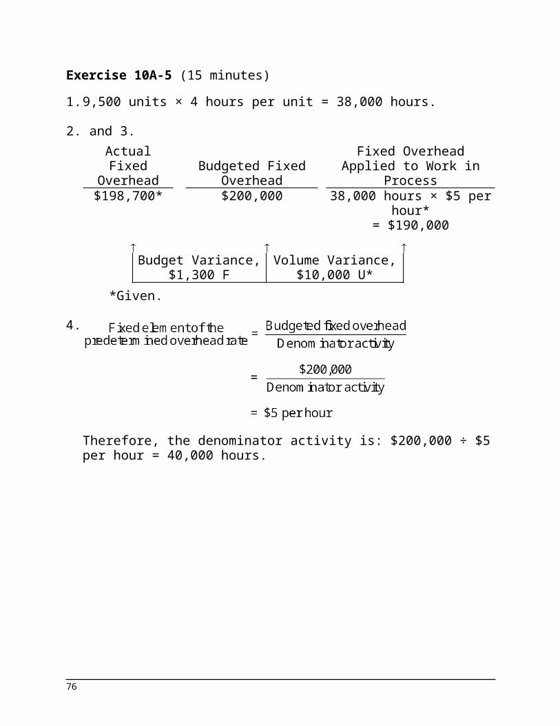
Exercise 10A-5 (15 minutes)1. 9,500 units × 4 hours per unit = 38,000 hours.
2. and 3.Actual Fixed Overhead
Budgeted Fixed Overhead
Fixed Overhead Applied to Work in Process
$198,700* $200,000 38,000 hours × $5 per hour*
= $190,000
Budget Variance,$1,300 F
Volume Variance,$10,000 U*
*Given.
4.
Therefore, the denominator activity is: $200,000 ÷ $5 per hour = 40,000 hours.
61
Exercise 10A-6 (15 minutes)1.
Variable element: ($1.90 per DLH × 30,000 DLHs) ÷ 30,000 DLHs = $57,000 ÷ 30,000 DLHs = $1.90 per DLH
Fixed element: $168,000 ÷ 30,000 DLHs = $5.60 per DLH
2. Direct materials, 2.5 yards × $8.60 per yard............ $21.50Direct labor, 3 DLHs* × $12.00 per DLH.................... 36.00Variable manufacturing overhead, 3 DLHs × $1.90
per DLH................................................................... 5.70Fixed manufacturing overhead, 3 DLHs × $5.60 per
DLH......................................................................... 16.80 Total standard cost per unit....................................... $80.00
*30,000 DLHs ÷ 10,000 units = 3 DLHs per unit.
62
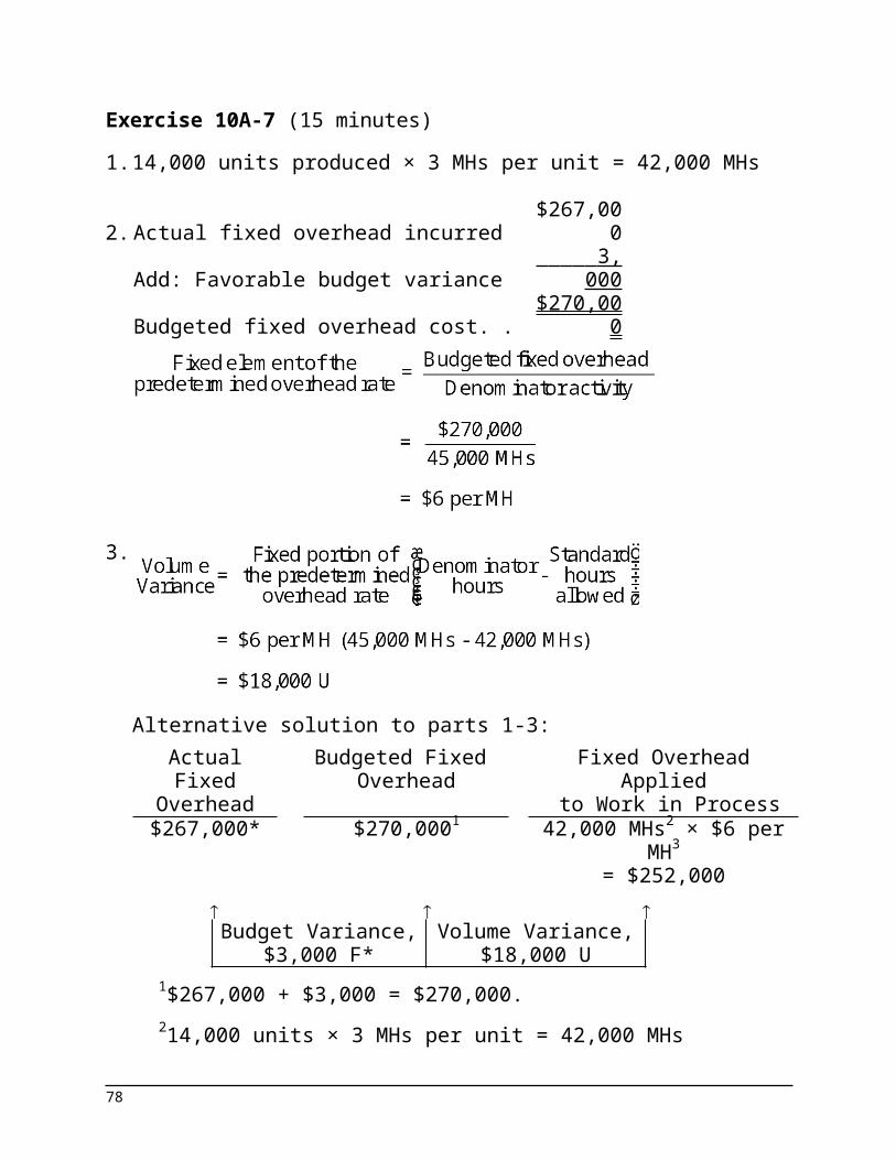
Exercise 10A-7 (15 minutes)1. 14,000 units produced × 3 MHs per unit = 42,000 MHs
2. Actual fixed overhead incurred..........$267,00
0Add: Favorable budget variance........ 3,000
Budgeted fixed overhead cost...........$270,00
0
3.
Alternative solution to parts 1-3:Actual Fixed Overhead
Budgeted Fixed Overhead
Fixed Overhead Applied to Work in Process
$267,000* $270,0001 42,000 MHs2 × $6 per MH3
= $252,000
Budget Variance, $3,000 F*
Volume Variance, $18,000 U
1$267,000 + $3,000 = $270,000.214,000 units × 3 MHs per unit = 42,000 MHs3$270,000 ÷ 45,000 denominator MHs = $6 per MH*Given.
63
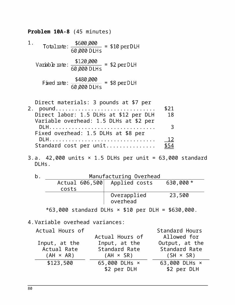
Problem 10A-8 (45 minutes)1.
2. Direct materials: 3 pounds at $7 per pound. . $21Direct labor: 1.5 DLHs at $12 per DLH.......... 18Variable overhead: 1.5 DLHs at $2 per DLH. . 3Fixed overhead: 1.5 DLHs at $8 per DLH....... 12 Standard cost per unit................................... $54
3. a. 42,000 units × 1.5 DLHs per unit = 63,000 standard DLHs.
b. Manufacturing OverheadActual costs
606,500 Applied costs 630,000 *
Overapplied overhead
23,500
*63,000 standard DLHs × $10 per DLH = $630,000.
4. Variable overhead variances:Actual Hours of
Input, at the Actual Rate
Actual Hours of Input, at the
Standard Rate
Standard Hours Allowed for Output,
at the Standard Rate
(AH × AR) (AH × SR) (SH × SR)$123,500 65,000 DLHs ×
$2 per DLH63,000 DLHs ×
$2 per DLH= $130,000 = $126,000
Rate Variance,
$6,500 FEfficiency Variance,
$4,000 U
64
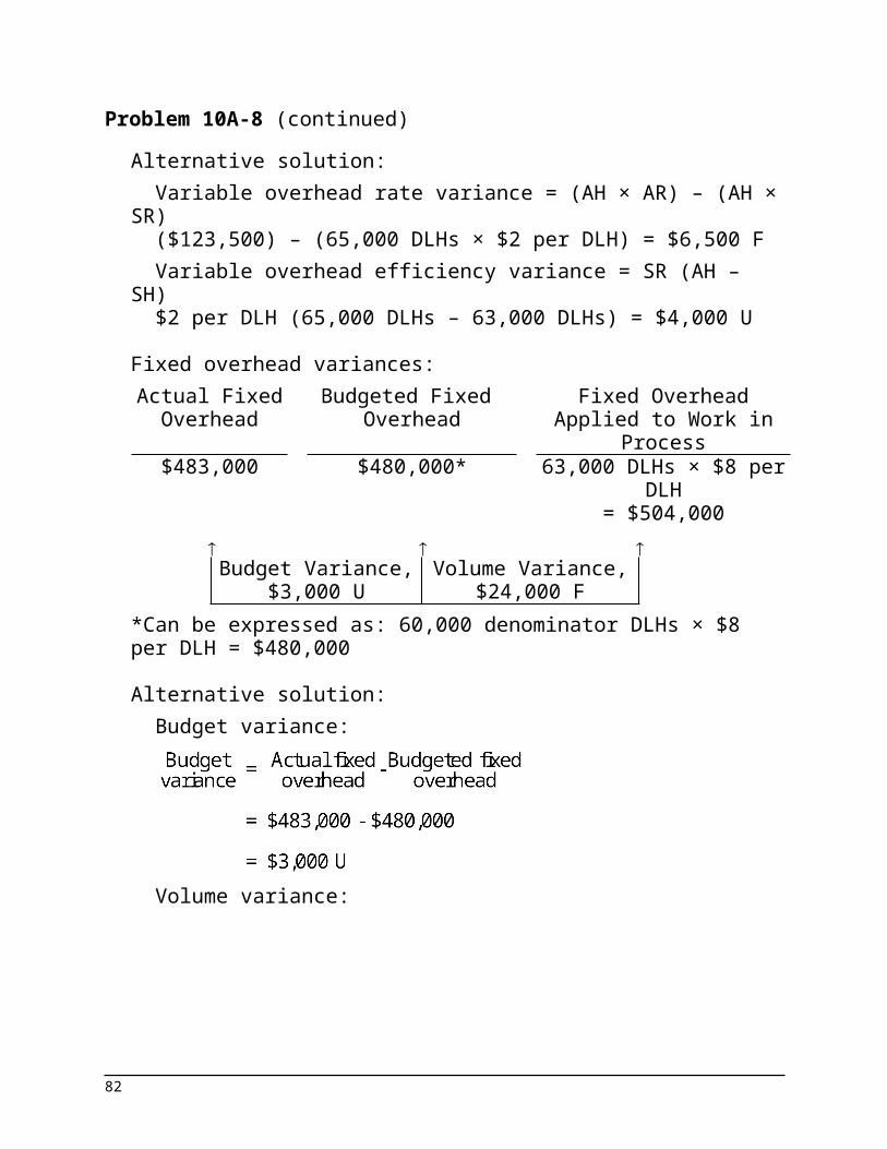
Problem 10A-8 (continued)Alternative solution:
Variable overhead rate variance = (AH × AR) – (AH × SR)($123,500) – (65,000 DLHs × $2 per DLH) = $6,500 FVariable overhead efficiency variance = SR (AH – SH) $2 per DLH (65,000 DLHs – 63,000 DLHs) = $4,000 U
Fixed overhead variances:Actual Fixed Overhead
Budgeted Fixed Overhead
Fixed OverheadApplied to Work in
Process$483,000 $480,000* 63,000 DLHs × $8 per
DLH= $504,000
Budget Variance,
$3,000 UVolume Variance,
$24,000 F*Can be expressed as: 60,000 denominator DLHs × $8 per DLH = $480,000
Alternative solution:Budget variance:
Volume variance:
65

Problem 10A-8 (continued)The company’s overhead variances can be summarized as follows:
Variable overhead:
Rate variance.............................$
6,500 FEfficiency variance..................... 4,000 U
Fixed overhead:Budget variance........................ 3,000 UVolume variance........................ 24,000 F
Overapplied overhead—see part 3
$23,500 F
5. Only the volume variance would have changed. It would have been unfavorable because the standard DLHs allowed for the year’s production (63,000 DLHs) would have been less than the denominator DLHs (65,000 DLHs).
66
Problem 10A-9 (45 minutes)1.
2. 32,000 standard hours × $8.50 per hour = $272,000.
3. Variable overhead variances:Actual Hours of
Input, at the Actual Rate
Actual Hours of Input, at the
Standard Rate
Standard Hours Allowed for Output,
at the Standard Rate
(AH × AR) (AH × SR) (SH × SR)$78,000 30,000 hours ×
$2.50 per hour32,000 hours ×$2.50 per hour
= $75,000 = $80,000
Rate Variance,$3,000 U
Efficiency Variance,$5,000 F
Alternative solution:Variable overhead rate variance = (AH × AR) – (AH × SR)($78,000) – (30,000 hours × $2.50 per hour) = $3,000 UVariable overhead efficiency variance = SR (AH – SH)$2.50 per hour (30,000 hours – 32,000 hours) = $5,000 F
67
Problem 10A-9 (continued)Fixed overhead variances:Actual Fixed Overhead
Budgeted Fixed Overhead
Fixed Overhead Applied to Work in Process
$209,400 $210,000 32,000 hours ×$6 per hour = $192,000
Budget Variance,
$600 FVolume Variance,
$18,000 U
Alternative solution:Budget variance:
Volume variance:
Verification:Variable overhead rate variance. $ 3,000 UVariable overhead efficiency
variance............................ 5,000F
Fixed overhead budget variance. 600 FFixed overhead volume variance 18,000 UUnderapplied overhead............... $15,400 U
68
Problem 10A-9 (continued)4. Variable overhead
Rate variance: This variance includes both price and quantity elements. The overhead spending variance reflects differences between actual and standard prices for variable overhead items. It also reflects differences between the amounts of variable overhead inputs that were actually used and the amounts that should have been used for the actual output of the period. Because the variable overhead spending variance is unfavorable, either too much was paid for variable overhead items or too many of them were used.Efficiency variance: The term “variable overhead efficiency variance” is a misnomer, because the variance does not measure efficiency in the use of overhead items. It measures the indirect effect on variable overhead of the efficiency or inefficiency with which the activity base is utilized. In this company, the activity base is labor-hours. If variable overhead is really proportional to labor-hours, then more effective use of labor-hours has the indirect effect of reducing variable overhead. Because 2,000 fewer labor-hours were required than indicated by the labor standards, the indirect effect was presumably to reduce variable overhead spending by about $5,000 ($2.50 per hour × 2,000 hours).
Fixed overheadBudget variance: This variance is simply the difference between the budgeted fixed cost and the actual fixed cost. In this case, the variance is favorable which indicates that actual fixed costs were lower than anticipated in the budget.Volume variance: This variance occurs as a result of actual activity being different from the denominator activity in the predetermined overhead rate. In this case, the variance is unfavorable, so actual activity was less than the denominator activity. It is difficult to place much of a meaningful economic interpretation on this variance. It tends to be large, so it often swamps the other, more meaningful variances if they are simply netted against each other.
69

Problem 10A-10 (45 minutes)1. Direct materials price and quantity variances:
Materials price variance = AQ (AP – SP)64,000 feet ($8.55 per foot – $8.45 per foot) = $6,400 UMaterials quantity variance = SP (AQ – SQ) $8.45 per foot (64,000 feet – 60,000 feet*) = $33,800 U
*30,000 units × 2 feet per unit = 60,000 feet
2. Direct labor rate and efficiency variances:Labor rate variance = AH (AR – SR)43,500 DLHs ($15.80 per DLH – $16.00 per DLH) = $8,700 FLabor efficiency variance = SR (AH – SH)$16.00 per DLH (43,500 DLHs – 42,000 DLHs*) = $24,000 U
*30,000 units × 1.4 DLHs per unit = 42,000 DLHs
3. a. Variable overhead spending and efficiency variances:Actual Hours of
Input, at the Actual Rate
Actual Hours of Input, at the
Standard Rate
Standard Hours Allowed for
Output, at the Standard Rate
(AH × AR) (AH × SR) (SH × SR)$108,000 43,500 DLHs
× $2.50 per DLH42,000 DLHs
× $2.50 per DLH= $108,750 = $105,000
Rate Variance,
$750 FEfficiency Variance,
$3,750 U
Alternative solution:Variable overhead rate variance = (AH × AR) – (AH × SR)($108,000) – (43,500 DLHs × $2.50 per DLH) = $750 FVariable overhead efficiency variance = SR (AH – SH)$2.50 per DLH (43,500 DLHs – 42,000 DLHs) = $3,750 U
70
Problem 10A-10 (continued)b. Fixed overhead budget and volume variances:Actual Fixed Overhead
Budgeted Fixed Overhead
Fixed Overhead Applied to Work in Process
$211,800 $210,000* 42,000 DLHs × $6 per DLH
= $252,000
Budget Variance,$1,800 U
Volume Variance,$42,000 F
*As originally budgeted. This figure can also be expressed as: 35,000 denominator DLHs × $6 per DLH = $210,000.
Alternative solution:Budget variance:
Volume variance:
71

Problem 10A-10 (continued)4. The total of the variances would be:
Direct materials variances:Price variance........................................ $ 6,400 UQuantity variance.................................. 33,800 U
Direct labor variances:Rate variance........................................ 8,700 FEfficiency variance................................ 24,000 U
Variable manufacturing overhead variances:Rate variance........................................ 750 FEfficiency variance................................ 3,750 U
Fixed manufacturing overhead variances:Budget variance.................................... 1,800 UVolume variance.................................... 42,000 F
Total of variances..................................... $18,300 UNote that the total of the variances agrees with the $18,300 variance mentioned by the president.It appears that not everyone should be given a bonus for good cost control. The materials quantity variance and the labor efficiency variance are 6.7% and 3.6%, respectively, of the standard cost allowed and thus would warrant investigation.The company’s large unfavorable variances (for materials quantity and labor efficiency) do not show up more clearly because they are offset by the favorable volume variance. This favorable volume variance is a result of the company operating at an activity level that is well above the denominator activity level used to set predetermined overhead rates. (The company operated at an activity level of 42,000 standard hours; the denominator activity level set at the beginning of the year was 35,000 hours.) As a result of the large favorable volume variance, the unfavorable quantity and efficiency variances have been concealed in a small “net” figure. The large favorable volume variance may have been achieved by building up inventories.
72
Problem 10A-11 (30 minutes)1. Direct materials, 3 yards × $4.40 per yard................... $13.20
Direct labor, 1 DLH × $12.00 per DLH........................... 12.00Variable manufacturing overhead, 1 DLH × $5.00 per
DLH*............................................................................ 5.00Fixed manufacturing overhead, 1 DLH × $11.80 per
DLH**.......................................................................... 11.80 Standard cost per unit................................................... $42.00
*$25,000 ÷ 5,000 DLHs = $5.00 per
DLH.
**$59,000 ÷ 5,000 DLHs = $11.80 per
DLH.
2. Materials variances:Materials price variance = AQ (AP – SP)24,000 yards ($4.80 per yard – $4.40 per yard) = $9,600 UMaterials quantity variance = SP (AQ – SQ)$4.40 per yard (18,500 yards – 18,000 yards*) = $2,200 U
*6,000 units × 3 yards per unit = 18,000 yards
Labor variances:Labor rate variance = AH (AR – SR)5,800 DLHs ($13.00 per DLH – $12.00 per DLH) = $5,800 ULabor efficiency variance = SR (AH – SH)$12.00 per DLH (5,800 DLHs – 6,000 DLHs*) = $2,400 F
*6,000 units × 1 DLH per unit = 6,000 DLHs
73

Problem 10A-11 (continued)3. Variable overhead variances:
Actual DLHs of Input, at the Actual Rate
Actual DLHs of Input, at the
Standard Rate
Standard DLHs Allowed for
Output, at the Standard Rate
(AH × AR) (AH × SR) (SH × SR)$29,580 5,800 DLHs
× $5.00 per DLH6,000 DLHs
× $5.00 per DLH= $29,000 = $30,000
Rate Variance,
$580 UEfficiency Variance,
$1,000 FSpending Variance,
$420 F
Alternative solution for the variable overhead variances:Variable overhead rate variance = (AH × AR) – (AH × SR)($29,580) – (5,800 DLHs × $5.00 per DLH) = $580 UVariable overhead efficiency variance = SR (AH – SH)$5.00 per DLH (5,800 DLHs – 6,000 DLHs) = $1,000 F
Fixed overhead variances:
Actual Fixed Overhead
Budgeted Fixed Overhead
Fixed Overhead Applied to
Work in Process$60,400 $59,000 6,000 DLHs
× $11.80 per DLH= $70,800
Budget Variance,
$1,400 UVolume Variance,
$11,800 F
74

Problem 10A-11 (continued)Alternative approach to the budget variance:
Alternative approach to the volume variance:
4. The choice of a denominator activity level affects standard unit costs in that the higher the denominator activity level chosen, the lower standard unit costs will be. The reason is that the fixed portion of overhead costs is spread over more units as the denominator activity rises.The volume variance cannot be controlled by controlling spending. The volume variance simply reflects whether actual activity was greater than or less than the denominator activity. Thus, the volume variance is controllable only through activity.
75
Problem 10A-12 (45 minutes)1. and 2. Per Direct Labor-Hour
Variable Fixed Total
Denominator of 30,000 DLHs:$135,000 ÷ 30,000 DLHs............ $4.50 $ 4.50$270,000 ÷ 30,000 DLHs............ $9.00 9.00
Total predetermined rate............... $13.50
Denominator of 40,000 DLHs:$180,000 ÷ 40,000 DLHs............ $4.50 $ 4.50$270,000 ÷ 40,000 DLHs............ $6.75 6.75
Total predetermined rate............... $11.25
3.Denominator Activity:
30,000 DLHsDenominator Activity:
40,000 DLHsDirect materials, 4 feet
× $8.75 per foot....... $35.00 Same......................... $35.00Direct labor, 2 DLHs ×
$15 per DLH.............. 30.00 Same......................... 30.00Variable overhead, 2
DLHs × $4.50 per DLH........................... 9.00 Same......................... 9.00
Fixed overhead, 2 DLHs × $9.00 per DLH........................... 18.00
Fixed overhead, 2 DLHs × $6.75 per DLH......................... 13.50
Standard cost per unit. $92.00Standard cost per
unit......................... $87.50
4. a. 18,000 units × 2 DLHs per unit = 36,000 standard DLHs.
b. Manufacturing OverheadActual costs 446,400 Applied costs 486,000 *
Overapplied overhead 39,600
*36,000 standard DLHs × $13.50 predetermined rate per DLH = $486,000.
76

Problem 10A-12 (continued)c. Variable overhead variances:
Actual DLHs of Input, at the Actual Rate
Actual DLHs of Input, at the
Standard Rate
Standard DLHs Allowed for
Output, at the Standard Rate
(AH × AR) (AH × SR) (SH × SR)$174,800 38,000 DLHs ×
$4.50 per DLH36,000 DLHs ×$4.50 per DLH
= $171,000 = $162,000
Rate Variance,$3,800 U
Efficiency Variance,$9,000 U
Alternative solution:Variable overhead rate variance = (AH × AR) – (AH × SR)($174,800) – (38,000 DLHs × $4.50 per DLH) = $3,800 UVariable overhead efficiency variance = SR (AH – SH)$4.50 per DLH (38,000 DLHs – 36,000 DLHs) = $9,000 U
Fixed overhead variances:Actual Fixed Overhead
Budgeted Fixed Overhead
Fixed Overhead Applied to Work in Process
$271,600 $270,000* 36,000 DLHs × $9 per DLH
= $324,000
Budget Variance,$1,600 U
Volume Variance,$54,000 F
*Can be expressed as: 30,000 denominator DLHs × $9 per DLH = $270,000.
77
Problem 10A-12 (continued)Alternative solution:
Budget variance:
Volume variance:
Summary of variances:Variable overhead rate variance......... $ 3,800 UVariable overhead efficiency variance 9,000 UFixed overhead budget variance......... 1,600 UFixed overhead volume variance......... 54,000 FOverapplied overhead......................... $39,600 F
78

Problem 10A-12 (continued)5. The major disadvantage of using normal activity is the large
volume variance that ordinarily results. This occurs because the denominator activity used to compute the predetermined overhead rate is different from the activity level that is anticipated for the period. In the case at hand, the company has used a long-run normal activity figure of 30,000 DLHs to compute the predetermined overhead rate, whereas activity for the period was expected to be 40,000 DLHs. This has resulted in a large favorable volume variance that may be difficult for management to interpret. In addition, the large favorable volume variance in this case has masked the fact that the company did not achieve the budgeted level of activity for the period. The company had planned to work 40,000 DLHs, but managed to work only 36,000 DLHs (at standard). This unfavorable result is concealed due to using a denominator figure that is out of step with current activity.On the other hand, using long-run normal activity as the denominator results in unit costs that are stable from year to year. Thus, management’s decisions are not clouded by unit costs that jump up and down as the activity level rises and falls.
79
Appendix 11BJournal Entries to Record Variances
Exercise 10B-1 (20 minutes)1. The general ledger entry to record the purchase of materials
for the month is:Raw Materials
(12,000 meters at $3.25 per meter)........... 39,000Materials Price Variance
(12,000 meters at $0.10 per meter F) 1,200Accounts Payable
(12,000 meters at $3.15 per meter)... 37,800
2. The general ledger entry to record the use of materials for the month is:
Work in Process (10,000 meters at $3.25 per meter)........... 32,500
Materials Quantity Variance(500 meters at $3.25 per meter U)............. 1,625
Raw Materials (10,500 meters at $3.25 per meter)... 34,125
3. The general ledger entry to record the incurrence of direct labor cost for the month is:
Work in Process (2,000 hours at $12.00 per hour)........................................................... 24,000
Labor Rate Variance (1,975 hours at $0.20 per hour U).............. 395
Labor Efficiency Variance (25 hours at $12.00 per hour F).......... 300
Wages Payable (1,975 hours at $12.20 per hour)........ 24,095
80

Exercise 10B-2 (45 minutes)1. a.
Actual Quantity of Input, at Actual Price
Actual Quantity of Input, at
Standard Price
Standard Quantity Allowed for Output,
at Standard Price(AQ × AP) (AQ × SP) (SQ × SP)
10,000 yards ×$13.80 per yard
10,000 yards ×$14.00 per yard
7,500 yards* ×$14.00 per yard
= $138,000 = $140,000 = $105,000
Price Variance,$2,000 F8,000 yards × $14.00 per yard
= $112,000
Quantity Variance, $7,000 U
*3,000 units × 2.5 yards per unit = 7,500 yards
Alternatively, the variances can be computed using the formulas:
Materials price variance = AQ (AP – SP)10,000 yards ($13.80 per yard – $14.00 per yard) = $2,000 FMaterials quantity variance = SP (AQ – SQ)$14.00 per yard (8,000 yards – 7,500 yards) = $7,000 U
81
Exercise 10B-2 (continued)b. The journal entries would be:
Raw Materials (10,000 yards × 14.00 per yard)........... 140,000
Materials Price Variance (10,000 yards × $0.20 per yard F) 2,000
Accounts Payable (10,000 yards × $13.80 per yard). 138,000
Work in Process (7,500 yards × $14.00 per yard)........... 105,000
Materials Quantity Variance (500 yards U × $14.00 per yard)........... 7,000
Raw Materials (8,000 yards × $14.00 per yard)... 112,000
2. a.Actual Hours of
Input, at the Actual Rate
Actual Hours of Input, at the
Standard Rate
Standard Hours Allowed for Output,
at the Standard Rate
(AH × AR) (AH × SR) (SH × SR)5,000 hours ×$8.00 per hour
4,800 hours* ×$8.00 per hour
$43,000 = $40,000 = $38,400
Rate Variance,$3,000 U
Efficiency Variance,$1,600 U
Spending Variance,$4,600 U
*3,000 units × 1.6 hours per unit = 4,800 hours
82

Exercise 10B-2 (continued)Alternative Solution:
Labor rate variance = AH (AR – SR)5,000 hours ($8.60 per hour* – $8.00 per hour) = $3,000 U
*$43,000 ÷ 5,000 hours = $8.60 per hourLabor efficiency variance = SR (AH – SH)$8.00 per hour (5,000 hours – 4,800 hours) = $1,600 U
b. The journal entry would be:Work in Process
(4,800 hours × $8.00 per hour)............... 38,400Labor Rate Variance
(5,000 hours × $0.60 per hour U)........... 3,000Labor Efficiency Variance
(200 hours U × $8.00 per hour).............. 1,600Wages Payable
(5,000 hours × $8.60 per hour).......43,00
0
3. The entries are: entry (a), purchase of materials; entry (b), issue of materials to production; and entry (c), incurrence of direct labor cost.
Raw Materials Work in Process(a) 140,000 (b) 112,000 (b) 105,000Bal.* 28,000 (c) 38,400
Accounts Payable Wages Payable(a) 138,000 (c) 43,000
Materials Price Variance Materials Quantity Variance(a) 2,000 (b) 7,000
Labor Rate Variance Labor Efficiency Variance(c) 3,000 (c) 1,600
*2,000 yards of material at a standard cost of $14.00 per yard
83
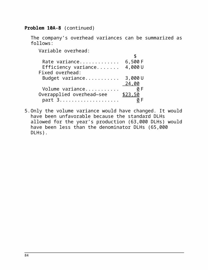
Problem 10B-3 (60 minutes)1. a.
Actual Quantity of Input, at Actual
Price
Actual Quantity of Input, at
Standard Price
Standard Quantity Allowed for Output, at Standard Price
(AQ × AP) (AQ × SP) (SQ × SP)32,000 feet ×$4.80 per foot
32,000 feet ×$5.00 per foot
29,600 feet* ×$5.00 per foot
= $153,600 = $160,000 = $148,000
Price Variance,$6,400 F
Quantity Variance,$12,000 U
Spending Variance, $5,600 U
*8,000 footballs × 3.7 ft. per football = 29,600 feet
Alternatively, the variances can be computed using the formulas:
Materials price variance = AQ (AP – SP)32,000 feet ($4.80 per foot – $5.00 per foot) = $6,400 FMaterials quantity variance = SP (AQ – SQ)$5.00 per foot (32,000 feet – 29,600 feet) = $12,000 U
b.Raw Materials (32,000 feet × $5.00 per
foot)...................................................... 160,000Materials Price Variance
(32,000 feet × $0.20 per foot F).. . 6,400Accounts Payable
(32,000 feet × $4.80 per foot)...... 153,600Work in Process
(29,600 feet × $5.00 per foot).............. 148,000Materials Quantity Variance
(2,400 feet U × $5.00 per foot)............. 12,000Raw Materials
(32,000 feet × $5.00 per foot)...... 160,000
84
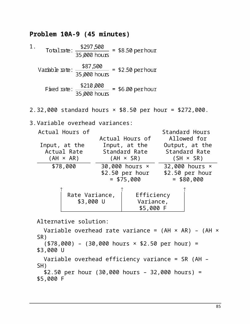
Problem 10B-3 (continued)2. a.
Actual Hours of Input, at the Actual Rate
Actual Hours of Input, at the
Standard Rate
Standard Hours Allowed for
Output, at the Standard Rate
(AH × AR) (AH × SR) (SH × SR)6,400 hours* ×$8.00 per hour
6,400 hours ×$7.50 per hour
7,200 hours** ×$7.50 per hour
= $51,200 = $48,000 = $54,000
Rate Variance,$3,200 U
Efficiency Variance,$6,000 F
Spending Variance,$2,800 F
* 8,000 footballs × 0.8 hours per football = 6,400 hours
** 8,000 footballs × 0.9 hours per football = 7,200 hours
Alternatively, the variances can be computed using the formulas:
Labor rate variance = AH (AR – SR)6,400 hours ($8.00 per hour – $7.50 per hour) = $3,200 ULabor efficiency variance = SR (AH – SH)$7.50 per hour (6,400 hours – 7,200 hours) = $6,000 F
b.Work in Process (7,200 hours × $7.50 per
hour).........................................................54,00
0Labor Rate Variance
(6,400 hours × $0.50 per hour U)............. 3,200Labor Efficiency Variance
(800 hours F × $7.50 per hour) ........ 6,000Wages Payable
(6,400 hours × $8.00 per hour)........51,20
0
85
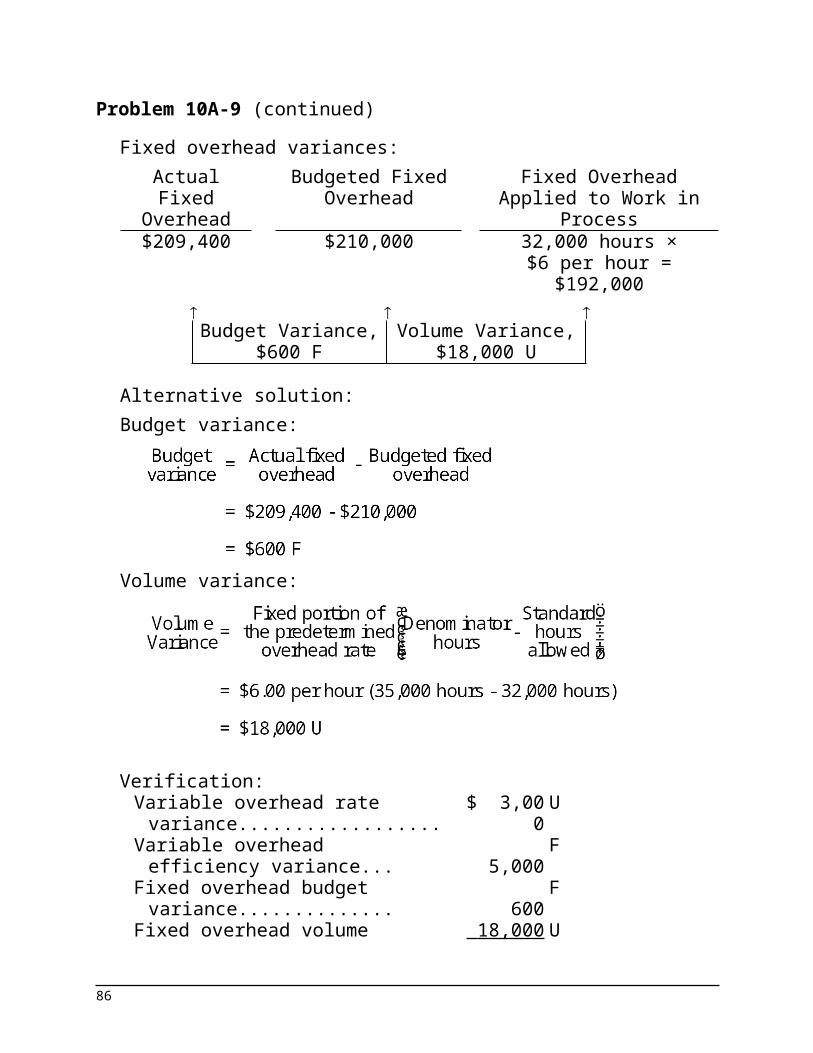
Problem 10B-3 (continued)3. Actual Hours of
Input, at the Actual Rate
Actual Hours of Input, at the
Standard Rate
Standard Hours Allowed for
Output, at the Standard Rate
(AH × AR) (AH × SR) (SH × SR)6,400 hours ×$2.75 per hour
6,400 hours ×$2.50 per hour
7,200 hours ×$2.50 per hour
= $17,600 = $16,000 = $18,000
Rate Variance,$1,600 U
Efficiency Variance,$2,000 F
Spending Variance, $400 F
Alternatively, the variances can be computed using the formulas:
Variable overhead rate variance = AH (AR – SR)6,400 hours ($2.75 per hour – $2.50 per hour) = $1,600 UVariable overhead efficiency variance = SR (AH – SH)$2.50 per hour (6,400 hours – 7,200 hours) = $2,000 F
4. No. He is not correct in his statement. The company has a large, unfavorable materials quantity variance that should be investigated. Also, the overhead rate variance equals 10% of standard, which should also be investigated.It appears that the company’s strategy to increase output by giving raises was effective. Although the raises resulted in an unfavorable rate variance, this variance was more than offset by a large, favorable efficiency variance.
86
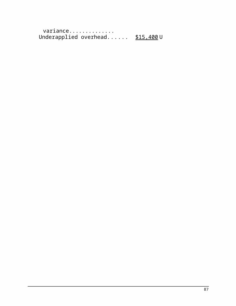
Problem 10B-3 (continued)5. The variances have many possible causes. Some of the more
likely causes include the following:
Materials variances:Favorable price variance: Good price, inferior quality materials, unusual discount due to quantity purchased, drop in market price, less costly method of freight, outdated or inaccurate standards.Unfavorable quantity variance: Carelessness, poorly adjusted machines, unskilled workers, inferior quality materials, outdated or inaccurate standards.
Labor variances:Unfavorable rate variance: Use of highly skilled workers, change in pay scale, overtime, outdated or inaccurate standards.Favorable efficiency variance: Use of highly skilled workers, high-quality materials, new equipment, outdated or inaccurate standards.
Variable overhead variances:Unfavorable rate variance: Increase in costs, waste, theft, spillage, purchases in uneconomical lots, outdated, or inaccurate standards.Favorable efficiency variance: Same as for labor efficiency variance.
87
Problem 10B-4 (75 minutes)1. a. Before the variances can be computed, we must first
compute the standard and actual quantities of material per hockey stick. The computations are:
Direct materials added to work in process (a).............................................
$115,200
Standard direct materials cost per foot (b).......................................................... $3.00
Standard quantity of direct materials (a) ÷ (b)....................................................... 38,400 feet
Standard quantity of direct materials (a). 38,400 feetNumber of sticks produced (b)................. 8,000Standard quantity per stick (a) ÷ (b)........ 4.8 feet
Actual quantity of direct materials used per stick last year:4.8 feet + 0.2 feet = 5.0 feet.
With these figures, the variances can be computed as follows:Actual Quantity
of Input, at Actual Price
Actual Quantity of Input, at Standard
Price
Standard Quantity Allowed for Output, at
Standard Price
(AQ × AP) (AQ × SP) (SQ × SP)60,000 feet ×$3.00 per foot
38,400 feet ×$3.00 per foot
$174,000 = $180,000 = $115,200
Price Variance,$6,000 F40,000 feet* × $3.00 per foot
= $120,000
Quantity Variance, $4,800 U
*8,000 units × 5.0 feet per unit = 40,000 feet
88
Problem 10B-4 (continued)Alternatively, the variances can be computed using the formulas:
Materials price variance = AQ (AP – SP)60,000 feet ($2.90 per foot* – $3.00 per foot) = $6,000 F
*$174,000 ÷ 60,000 feet = $2.90 per footMaterials quantity variance = SP (AQ – SQ)$3.00 per foot (40,000 feet – 38,400 feet) = $4,800 U
b.Raw Materials (60,000 feet × $3.00 per
foot)..........................................................180,00
0Materials Price Variance
(60,000 feet × $0.10 per foot F).......... 6,000Accounts Payable
(60,000 feet × $2.90 per foot).............174,00
0Work in Process (38,400 feet × $3.00 per
foot)..........................................................115,20
0Materials Quantity Variance
(1,600 feet U × $3.00 per foot)................. 4,800Raw Materials (40,000 feet × $3.00 per
foot).....................................................120,00
0
89

Problem 10B-4 (continued)2. a. Before the variances can be computed, we must first
determine the actual direct labor hours worked for last year. This can be done through the variable overhead efficiency variance, as follows:
Variable overhead efficiency variance = SR (AH – SH)$1.30 per hour × (AH – 16,000 hours*) = $650 U$1.30 per hour × AH – $20,800 = $650**$1.30 per hour × AH = $21,450 AH = $21,450 ÷ $1.30 per hour AH = 16,500 hours * 8,000 units × 2.0 hours per unit = 16,000 hours** When used in the formula, an unfavorable variance is
positive.
We must also compute the standard rate per direct labor hour. The computation is:Labor rate variance = (AH × AR) – (AH × SR) $79,200 – (16,500 hours × SR) = $3,300 F$79,200 – 16,500 hours × SR = –$3,300*16,500 hours × SR = $82,500 SR = $82,500 ÷ 16,500 hours SR = $5.00 per hour* When used in the formula, a favorable variance is negative.
90
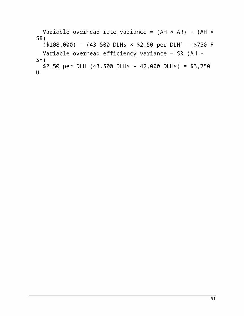
Problem 10B-4 (continued)Given these figures, the variances are:
Actual Hours of Input, at the Actual Rate
Actual Hours of Input, at the
Standard Rate
Standard Hours Allowed for Output,
at the Standard Rate
(AH × AR) (AH × SR) (SH × SR)16,500 hours ×$5.00 per hour
16,000 hours ×$5.00 per hour
$79,200 = $82,500 = $80,000
Rate Variance,$3,300 F
Efficiency Variance,$2,500 U
Spending Variance,$800 F
Alternatively, the variances can be computed using the formulas:
Labor rate variance = AH (AR – SR)16,500 hours ($4.80 per hour* – $5.00 per hour) = $3,300 F*79,200 ÷ 16,500 hours = $4.80 per hourLabor efficiency variance = SR (AH – SH)$5.00 per hour (16,500 hours – 16,000 hours) = $2,500 U
b. Work in Process (16,000 hours × $5.00 per hour).............. 80,000
Labor Efficiency Variance (500 hours U × $5.00 per hour)................ 2,500
Labor Rate Variance (16,500 hours × $0.20 per hour F)....... 3,300
Wages Payable (16,500 hours × $4.80 per hour).......... 79,200
91

Problem 10B-4 (continued)3. Actual Hours of
Input, at the Actual Rate
Actual Hours of Input, at the
Standard Rate
Standard Hours Allowed for Output,
at the Standard Rate
(AH × AR) (AH × SR) (SH × SR)16,500 hours ×$1.30 per hour
16,000 hours ×$1.30 per hour
$19,800 = $21,450 = $20,800
Rate Variance,$1,650 F
Efficiency Variance,$650 U
Spending Variance,$1,000 F
Alternatively, the variances can be computed using the formulas:
Variable overhead rate variance = AH (AR – SR)16,500 hours ($1.20 per hour* – $1.30 per hour) = $1,650 F
*$19,800 ÷ 16,500 hours = $1.20 per hourVariable overhead efficiency variance = SR (AH – SH)$1.30 per hour (16,500 hours – 16,000 hours) = $650 U
92

Problem 10B-4 (continued)4. For materials:
Favorable price variance: Decrease in outside purchase price; fortunate buy; inferior quality materials; unusual discounts due to quantity purchased; less costly method of freight; inaccurate standards.
Unfavorable quantity variance: Inferior quality materials; carelessness; poorly adjusted machines; unskilled workers; inaccurate standards.
For labor:Favorable rate variance: Unskilled workers (paid lower rates);
piecework; inaccurate standards.Unfavorable efficiency variance: Poorly trained workers; poor
quality materials; faulty equipment; work interruptions; fixed labor and insufficient demand to fill capacity; inaccurate standards.
For variable overhead:Favorable rate variance: Decrease in supplier prices; less usage
of lubricants or indirect materials than planned; inaccurate standards.
Unfavorable efficiency variance: See comments under direct labor efficiency variance above.
5.Standard
Quantity or Hours
Standard Price or Rate
Standard
CostDirect materials......... 4.8 feet $3.00 per foot $14.40Direct labor............... 2.0 hours $5.00 per hour 10.00Variable overhead..... 2.0 hours $1.30 per hour 2.60 Total standard cost.... $27.00
93
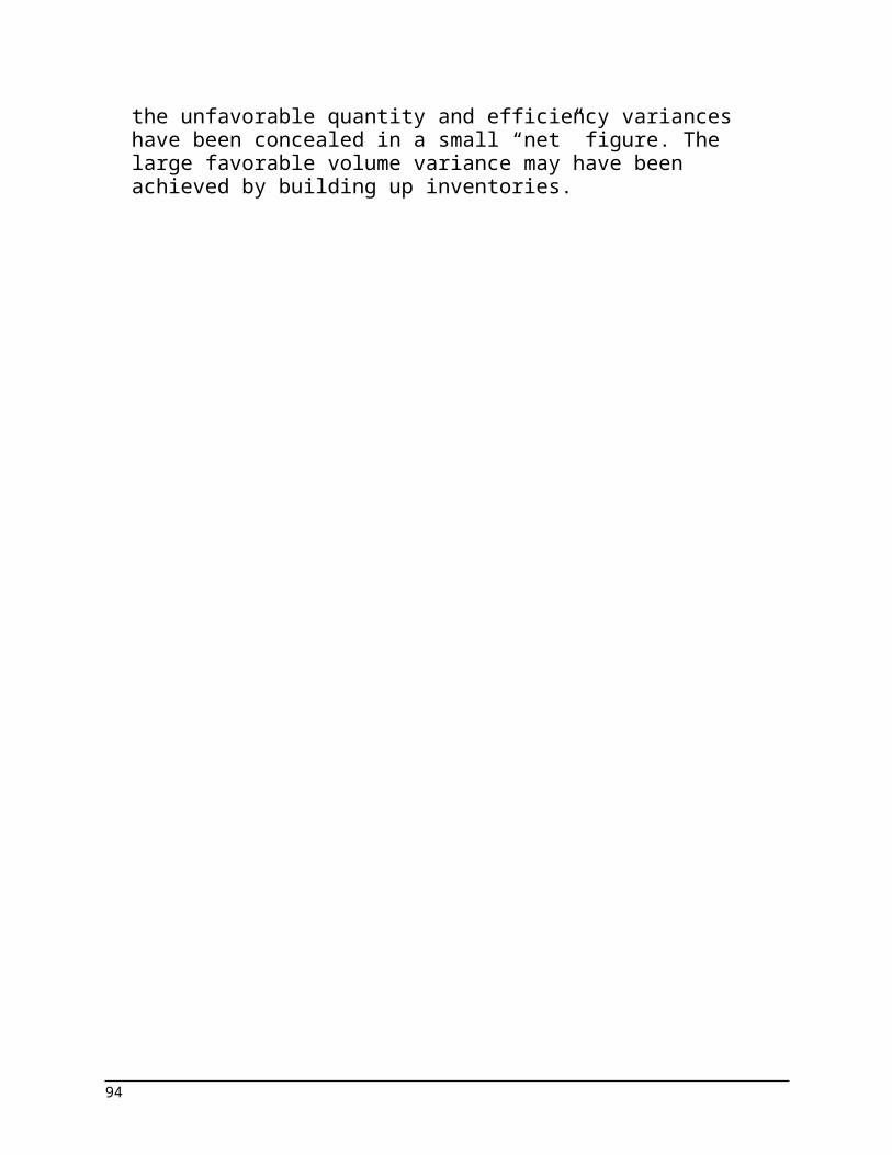
Case 10B-5 (30 minutes)This case may be difficult for some students to grasp because it requires looking at standard costs from an entirely different perspective. In this case, standard costs have been inappropriately used as a means to manipulate reported earnings rather than as a way to control costs.
1. Lansing has evidently set very loose standards in which the standard prices and standard quantities are far too high. This guarantees that favorable variances will ordinarily result from operations. If the standard costs are set artificially high, the standard cost of goods sold will be artificially high and thus the division’s net operating income will be depressed until the favorable variances are recognized. If Lansing saves the favorable variances, he can release just enough in the second and third quarters to show some improvement and then he can release all of the rest in the last quarter, creating the annual “Christmas present.”
2. Lansing should not be permitted to continue this practice for several reasons. First, it distorts the quarterly earnings for both the division and the company. The distortions of the division’s quarterly earnings are troubling because the manipulations may mask real signs of trouble. The distortions of the company’s quarterly earnings are troubling because they may mislead external users of the financial statements. Second, Lansing should not be rewarded for manipulating earnings. This sets a moral tone in the company that is likely to lead to even deeper trouble. Indeed, the permissive attitude of top management toward the manipulation of earnings may indicate the existence of other, even more serious, ethical problems in the company. Third, a clear message should be sent to division managers like Lansing that their job is to manage their operations, not their earnings. If they keep on top of operations and manage well, the earnings should take care of themselves.
94

Case 10B-5 (continued)3. Stacy Cummins does not have any easy alternatives available.
She has already taken the problem to the President, who was not interested. If she goes around the President to the Board of Directors, she will be putting herself in a politically difficult position with little likelihood that it will do much good if, in fact, the Board of Directors already knows what is going on.On the other hand, if she simply goes along, she will be violating the Credibility standard of ethical conduct for management accountants. The Home Security Division’s manipulation of quarterly earnings does distort the entire company’s quarterly reports. And the Credibility standard clearly stipulates that management accountants have a responsibility to “disclose all relevant information that could reasonably be expected to influence an intended user’s understanding of the reports, analyses, or recommendations.” Apart from the ethical issue, there is also a very practical consideration. If Merced Home Products becomes embroiled in controversy concerning questionable accounting practices, Stacy Cummins will be viewed as a responsible party by outsiders and her career is likely to suffer dramatically and she may even face legal problems.We would suggest that Ms. Cummins quietly bring the manipulation of earnings to the attention of the audit committee of the Board of Directors, carefully laying out in a non-confrontational manner the problems created by Lansing’s practice of manipulating earnings. If the President and the Board of Directors are still not interested in dealing with the problem, she may reasonably conclude that the best alternative is to start looking for another job.
95