chapter geological mapping

The Computer in Contemporary CartographyEdited by D. R. F. TaylorCo 1980 John Wiley & Sons Ltd

Chapter 8Geological Mapping by Computer

CHRISTOPHER GOLD

INTRODUCTION

Davis (1973), p. 298 states: ‘Maps are as important to earth scientists as theconventions for scales and notes are to the musician, for they are compact andefficient means of expressing relat ionships and details . Although maps are a familiarpart of every geologist’s t raining and work, surpris ingly l i t t le thought has gone intothe mechanics and philosophy of geologic map making.’ He then states that most ofthe work in this f ield is done by geographers, and gives various examples. One of thedifficult ies with this approach of merely accepting rather than developing techniquesis that many of the wide variety of map types that geologists use are uncommon inother discipl ines .

Maps are displays of i tems of information that have both and non-spatialcomponents-without both of these it is not possible to produce a true map. Datathat are not in suitable form must be transformed in order to make map productionpossible. Statistical data, for example, do not usually possess information about thelocation of each data point in space, but scatter plots or contour plots are frequentlygenerated from data of this type, by arbitrari ly considering two variables to represent‘east’ and ‘north’ and then either plotting data point locations or contouring thevalue of some other associated variable . A point to note is that , given points within ascatter diagram, it is often desirable to contour their density. This density is acontinuous variable expressing the number of points per unit area. Unfortunately,the resulting surface varies greatly with the sampling area chosen. Thistransformation from point locat ion to densi ty has been s tudied by various geologis ts ,in particular Ramsden ( 1975, and in press).

Perhaps surprisingly, one-dimensional maps are commonly used by geologists:the geological section is the basic tool of much field work. The direction is usuallyvertical and the mapped variable may be either categorical, as in stratigraphicsections showing the rock types and formations present in some locality, orcontinuous, as with electric log measurements of resistivity, etc., down a drill hole.Much geological work consists of taking these one-dimensional maps and correlat ingbetween them to produce two-dimensional cross-sections (Figure 8.1 A) which imply ,conceptually if not diagrammatically, three-dimensional models (Figure 8.1 B).

152 P R O G R E S S I N C O N T E M P O R A R Y C A R T O G R A P H Y

Alternatively, the three-dimensional model may be constructed by generatingcontour maps of each geological contact in turn.

O-

-1000

-2ooo~

-3000

-4oo0,

w

8.1 Wind River Basin, Wyoming, stratigraphic cross-section and block diagram(Harbrough and Merriam, I968 ; reproduced by permission of John Wiley & Sons, Inc.)

If only spatial information is present in a data set it may become necessary toeliminate one dimension by treating it as non-spatial for display purposes. Anexample is the case of a topographic map where east, north and verticalmeasurements are obtained for points on the atmosphere-l i thosphere contact . In thiscase the elevation information is t reated as non-spatial and displayed in various ways

G E O L O G I C A L M A P P I N G B Y C O M P U T E R 153

on the two-dimensional map sheet-perhaps by plotting spot elevations, colouringelevation zones or some other technique. I t is , of course, possible to choose a differentpair of map variables and draw a cross-section to the topographic surface, usuallywith the y-axis of the map representing the elevation.

Geologists basically study the earth, a three-dimensional object , and are frequentlyconcerned with the variation of one or many parameters within three-dimensionalspace. This differs markedly from political scientists, for example, who rarelyconsider the vertical variation in voting preferences! (Both groups, however, wouldfrequently like to be able to represent time as another spatial dimension.) Thisunderlying concern with what is happening in the third, undisplayed, spatialdimension is of great importance in some, if not all, branches of geology.Considerable use is made of mapped data containing no intr insic spat ial information ;for example, in examining how one measured chemical component in a set of rocksamples varies with changes in another component. Most maps make use of datawith only two spatial variables--examples of these are maps of the earth’s magneticfield, concentration of some economic mineral or element found in an area, or thetype of rock to be found in a particular geographic region. This last is perhaps whatmost people think of as a geological map. A classical example of this is shown inFigure 8.2, the first true geological map, drawn by William Smith and published in18 15 and showing the major rock units in England and Wales. Nevertheless, a littlethought will suggest that all of these examples are two-dimensional only because ofthe inability to collect samples far from the surface of the earth, not from limitationsin the display technique. Indeed, many maps are intended to facilitate the intuitiveestimation of variation in the third dimension, based on professional knowledge ofthe behaviour of the parameters displayed (see the discussion in Gold and Kilby,1978). This is especially true for maps displaying structure and lithology, wherestructural boundaries and plotted bedding orientat ions are designed to enhance thethree-dimensional model perceived by the compiling geologist.

Maps that are usually amenable to consideration as two-dimensional includemany maps (geomagnetic, gravitational, etc.) , geochemical maps (plot t ingthe concentration of some element measured in samples of soil, rock, or waterobtained near the earth-air or earth-water contact) and .facies maps (partitioningsome geological contact into zones with relatively homogeneous properties).Orientation and density maps wil l usual ly be two-dimensional as well . Depending onthe scale and the objectives of the study, ‘geological or, more properly, ‘ l ithological ’maps may be considered to be two-dimensional, but as previously. noted the thirddimension may be indicated ei ther by bedding orientat ion symbols or by the form ofthe geological contact, especially as i t relates to the topographic surface. Topographicmaps, structural contour maps, isopach maps, and other derivatives are of coursethree-dimensional in input, even if the vertical dimension must be treated as amapped variable for display. These map types, along with related discussions of datacapture and data base management, will be described under separate headings laterin this chapter.

P R O G R E S S I N C O N T E M P O R A R Y C A R T O G R A P H Y

8.2 Part of William Smith’s geological map of Britain, 18 15. Figure 1.7 (p. 10) in EarthHistory and flare Tectonics, 2nd Edn, by Carl K. Seifert and Leslie A. Sir-kin. Copyright 01979 by Carl K. Seifert and Leslie A. Sirkin. Reproduced by permission of Harper and Row,

Publishers, Inc

Perhaps it is worth making a comment here on the role of maps in geology. Theyare certainly a product-most geologists have produced maps. As well as outputthey are also input-all geologists have read maps ; many kinds of maps. Rather thanbeing attractive products to pass on to the end-user, most maps are an essential , andprimary, means of communication between geologists , and most are not expected to


be meaningful even to those geologists not concerned with the part icular topic underconsideration. Since relatively few maps are intended for immediate comprehensionby the general public, a high level of generalization is not usually desirable.Hopefully this explains, and even excuses, the great amount of detail found in manygeological maps.

Having mentioned the role of maps in geology, we come to the main purpose ofthis chapter-to discuss the role of the computer in producing geological maps, andin part icular how the advent of the computer has affected geological map production.The main details of these changes are described under each map type. In general, thefirst change produced by computer availability was the dramatic increase in thequantity of data points generated, with the consequent necessity to display them.This is still the driving force behind map automation. The first mapping techniquesdeveloped in response were contouring algorithms, and these are still the leadingmapping functions used. It is becoming evident, however, that some of the earlierand more inefficient approaches to contouring are beginning to show signs of wearunder the ever-increasing load of generated data.

Apart from contour mapping, the increasing volume of data has mainly generatedprograms for individual data point display (‘posting’) and statistical and other datatransformations. Of course, once it became easy to generate many maps from onedata set , many maps were requested. One offshoot of this is that i t is becoming morecommon to standardize the acquisition of field data by using coding forms, thusfacilitating data entry for computer generation of base maps that rapidly display theraw data for subsequent interpretation. It is now not unknown for the weekly mailplane to arrive at the bush camp to collect the week’s coding forms and deliver thelatest base maps.

The primary effect of computers has thus been to facil i tate the production of ever-increasing numbers of simple maps. In this way the geologist may more rapidlyreach the stage of data interpretation, where his comprehension of geologicalprocesses may help him to make meaningful decisions from the displayedinformation. Nevertheless much research is in progress in other directions, oftenwith the intention of computerizing or s tandardizing even more of the routine labourof the practising geologis t .

GEOPHYSICAL MAPS

Geophysical mapping involves the display of a wide variety of physical parameters,for example the earth’s gravitational field, the earth’s magnetic field (both strengthand orientation) and earthquake data. Also mapped, on a more local scale, areresistivity and self potential data and, even more commonly, seismic data for oilexploration. A wide variety of less common data types are also used.

Most of these measurement techniques have some features in common-largequanti t ies of data are accumulated by automatic means, usually along fl ight paths ortraverse l ines. The data processing is frequently sophist icated and beyond the scope


of this study. Nevertheless difficulties exist in the management and display of thelarge quantit ies of data of this type that are relevant here. The key point, however, isthat the display of large quantities of data necessitates the use of computer-basedmapping sys tems.

While many types of geophysical measurement are possible, examples will begiven for geomagnetic surveys (examining the earth’s magnetic field either forregional trends or local anomalies): gravity surveys (as above, but for thegravitational field); seismic ‘profiling’ to identify geological contacts by monitoringthe reflection of shock waves; and regional seismic studies to determine earthquakelocat ions .

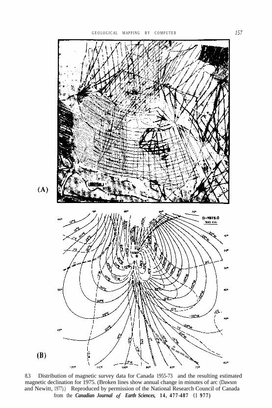
Dawson and Newitt (1977) produced a regional map of the earth’s magnetic fieldfor Canada, based on 5 1,133 data points (Figure 8.3~) for which the earth’s field hadbeen obtained in three perpendicular directions. These data were obtained from anon-going data collection process from 1900 to the present although, since all threecomponents of the earth’s f ield had to be measured at each location, the data pointsactually used were acquired between 1955 and 1974. Observations were obtainedeither from ground stations or, more recently and for the bulk of the data, from aerialsurveys.

Since this was a regional survey, concerned with field fluctuations of the order of1000 km in wavelength, it was estimated that a sixth-degree polynomial fit in eachquarter of the map area would display such features. In addition, since the earth’sfield varies with t ime, a cubic t ime component was used to adjust for data acquired atdifferent dates. The resulting charts were plotted for estimated 1975 values and acorrection applied to correct to sea-level elevation. These charts displayed D.(magnetic declination), H (horizontal intensity), Z (vertical intensity), I (magneticinclination) and F (total intensity). These parameters (which are merely differentways of displaying the orientation and intensity of the field calculated using theorthogonal x, y, and z vectors), were plotted using the regression coefficientsobtained independently for the x, y, and z components. Figure 8.3~ shows the mapfor magnetic declination.

Kearey ( 1977) described a gravity survey of the Central Labrador Trough,Northern Quebec. Average sample spacing was 5 km, with some detailed traverseshaving a spacing of 1.5 km or less. Regional and residual gravity fields wereestimated. The residual field was then related to the lithologic variation within theTrough.

Howells and Mackay ( 1977) performed a seismic reflection survey of MiramichiBay, New Brunswick. A more common type of survey uses the refraction technique,which determines the propagation velocity of seismic energy through rocks andsurficial sediments . Contrast ing l i thologies may be correlated with certain veloci t ies ,or velocity ranges, provided borehole control is available. This approach is the oneprimarily used in oil exploration. In the Miramichi study, however, the water depthand available equipment made a reflection survey more applicable.

The objective of the survey was to determine surficial sediment types and


(W

8.3 Distribution of magnetic survey data for Canada 1955-73 and the resulting estimatedmagnetic declination for 1975. (Broken lines show annual change in minutes of arc (Dawsonand Newitt, 1977).) Reproduced by permission of the National Research Council of Canada

from the Canadian Journal qf Earth Sciences, 14, 477-487 (I 977)


thicknesses in the area, and over 300 line kilometres of seismic profiling wasobtained. The equipment used consisted of a launch-mounted echo-sounder receiverwith the ‘boomer’ sound generator towed behind on a catamaran. Position fixing forthe survey was accomplished using a microwave system with three pairs of land-based slave stations. The overall position-fixing repeatability was about 10 m. Theinner part of the bay was less than 7 m deep; the outer part sloping, to 15 m.

In the presence of soft bottom muds a good reflection was received from theharder underlying material. Where the sediments were harder penetration was notachieved, but sea f loor roughness was used to dist inguish relat ively f lat sands fromthe rougher exposed bedrock. This interpretation was aided by several shallowboreholes. On the basis of these measurements various conclusions were made aboutthe geological history of the area.

Basham et al. (1977) examined the last data type we will consider under theheading of geophysics---the incidence of earthquakes. From the catalogue ofCanadian earthquakes, they extracted all those with epicentres north of 59 degrees oflatitude. Their objectives were to review what is known of the seismicity in northernCanada, and to comment on the spatial relationships between seismicity and othergeological and geophysical features. The data consisted of events monitored since1962, the first year a large enough number of seismographic stations weremaintained in the area to provide reasonably comprehensive coverage. They statethat the better-defined epicentres are probably located to within 50 km, with theworst having a location error of up to 100 km, depending on the distance to thenearest s tat ions. They then at tempted to relate the clustering of these observations tovarious other features and concluded that they may be explained by knowndeformational features, by sedimentary loading of the crust and by residualdisequilibrium due to crustal unloading at the time of the last major glacial retreat.

In evaluating the impact of the computer on the types of s tudies mentioned here, i tis clear that for the magnetic and gravity surveys the computer is a necessity tohandle the many thousands of data points acquired. Indeed, i t is probably true to saythat the abil i ty to acquire large quanti t ies of data grew from the same technology as,and because of the availability of, the ability to display the resulting information.Thus without computer-based mapping the projects in their present form would nothave been performed. In the seismic reflection and earthquake incidence studiessophist icated instrumentat ion was needed for data acquisi t ion, but the projects couldhave been completed without the use of computer cartography.

GEOCHEMICAL MAPS

Geochemistry, particularly in mineral exploration, is one of the oldest geologicalskills. Agricola, for example, in 1546, described six basic flavours of spring water,that were of use in determining mineral deposits. Indicator plants-species that grownear particular types of mineralization-have been known for a millennium. Placerexploration-panning for gold, tin, etc.-is also ancient. Geochemical exploration

G E O L O G I C A L M A P P I N G B Y C O M P U T E R

today is little different in this respect-lements are searched for in rock, soil,sediment, plant, and water samples. The main differences are in analyticinstrumentation, sampling methodology and data processing of the results. It is notcommonly realized how many geochemical analyses are, in fact, performed withmodern rapid analytic instrumentation. In the 197 l-72 year over 800,000 sampleswere analysed for at least one element in Canada, and over 300,000 in the U.S.A.Soil, rock, and stream sediment samples comprised the vast bulk of these rocksamples being more popular in the U.S.A. and soil samples in Canada, presumablydue to northern terrain types. Most of the other analyses were performed on waterand vegetat ion samples.

Sample collection has several aspects. I t is the job of the geochemist to determinethe best position in the stream bed or the best depth in the soil profile to collect asample. This should be based on his knowledge of the dispersion mechanisms of theelement or mineral for which he is searching. Another aspect concerns the spacing ofsamples--clearly, if samples are too far apart the target anomaly may well bemissed ; and if samples are too closely spaced considerable money is being wasted. Adecision must also be made as to what kind of sampling to perform-it may well bemuch cheaper to sample vegetat ion for elemental analysis than to dig a sui table holefor soil sampling. The number of elements to be analysed in each sample is anotherfactor in the economic equation, since several elements may correlate well together,or certain element combinations may indicate either a false anomaly (where theaccumulation of the target elements is merely due to the dispersion agents, such asground water) or strongly suggest a true one.

The manipulation and display of data after sample acquisi t ion and analysis is thefinal step. As might be expected from the cost of data acquisit ion, considerable effortis sometimes expended on this stage but, conversely, a surprisingly large number ofsurveys are satisfied with elementary processing techniques. This is, in part,explainable by the lack of consensus on methodology. In addit ion, survey objectivesmay be either regional geochemistry, where the objective is to observe the generalbehaviour of some component over appreciable distances, or explorationgeochemistry, where the objective is to determine anomalously high concentrationsof some mineral of economic interest. Since the concentration of the target materialfrequently varies greatly over even small distances, appreciable smoothing should beperformed prior to map production. For regional analysis, trend surface methods (seeDavis, 1973) are commonly used for computer-based estimation of smooth regionaltrends. In exploration geochemistry careful examination of the possible populationdistributions is necessary before areas possessing appreciable concentrations of thedesired material can be satisfactorily distinguished from the ‘background’ range ofexpected data values (Govett et al., 1975).

The first requirement of data examination is to determine the background andthreshold values for the region. These are defined as the average regional value andthe upper limit of regional variation exclusive of anomalous zones. This raises twopoints. First, a region has to be defined within which the background variation is


more or less homogeneous (this may be identifiable from other information, such asrock type). Second, an anomaly is defined as having values outside (usually above)the expected background variation, so the argument is circular-as indeed it is fordefining regions or domains as well. This is a major problem in cartographic work ingeology-the delineation of zones with similar properties. Determination of regionsor anomalies is not usually a major problem when mapping by hand-other aspectsof the data can be taken into account by the trained geologist. The advent ofcomputer analysis , however, rapidly demands the introduction of computer-assistedmapping, with a consequent demand to specify the cri teria more precisely. In theorythis is good, since i t forces objectivity. Nevertheless, in practice i t has merely deterredthe use of the computer on a production basis, since it appears to the untrainedindividual that much effort and statistical skill is needed merely to simulate the‘obvious’ manual interpretation.

The above remarks apply to both data posting-where anomalous values may beflagged automatically-or for contour maps. In the second case production of a maphonouring all data values is frequently undesirable, as the errors in sampling andanalysis may generate surface fluctuations that obscure the subregional behaviour.In stat is t ical terms, the correlat ion between neighbouring points is not very high. Formost purposes, it is necessary to filter or smooth the data.

Data smoothing occurs every time the mathematical surface generated from thedata fails to honour, or pass through, all the input points. This is a naturalconsequence of the gridding stage in most computer programmes, since therequirement that the surface passes through the interpolated values at the nodes ofwhat is usual ly a relat ively course intermediate grid precludes the possibi l i ty of theirpassing through the data points, especially if several occur in one cell . I t is necessaryin most cases to be able to control the extent of smoothing, and this may be achievedusing various approaches. For regularly spaced data on a grid, Robinson andCharlesworth (1975) used a Fourier filter to eliminate both excessively high and lowfrequencies. Their information was concerned with subsurface stratigraphy inwestern Canada, and for oil exploration purposes they wished to examine features afew kilometres in length that could possibly be buried reefs. Unfortunately controlledsmoothing of this type is not readily obtainable for irregularly spaced data.

Contouring is usually performed using an arbitrary grid over the map area andestimating elevations at each node. Clearly enlarging the grid spacing increases thesmoothing of the data . This necessi tates some interpolat ion method to est imate gridnode values from nearby data points. A typical method is the moving average, wherethe value at any location is a weighted average of the nearby points, closer pointsbeing weighted more heavily than more distant points. Two sources of deviation ofthe surface from the data values should be noted. First, if the weighting function issuch that at any data location any other data points contribute to the surface beinggenerated, then the surface will not pass precisely through the original data. Thisdepends on the weighting function itself. A weighting of 1 /d2, where d is thedistance between data location and grid node, will not produce any smoothing. A

GEOLOGICAL MAPPING BY COMPUTER 161

weighting of exp ( - d), on the other hand, will do so. If d = 0, the first case yields aninfinite weighting, while the second gives unity. Secondly, the very existence of anintermediate gr id smooths the data uncontrol lably, s ince data points not lying at gr idnodes will rarely be honoured.

To meet the need for smoothed maps two competing techniques have been used ingeology: trend surfaces and kriging. Trend surface analysis consists of fitting apolynomial of fixed order in x and y to the data, using conventional regressiontechniques. This has the advantage that t radit ional s tat is t ical techniques may be used,although it is assumed in the method that local fluctuations (the ‘error’ component)are uncorrelated. This is reasonable for errors in measurement of a geochemicalvariable, but is not correct for real small-scale or local variations. In addition, there isno foolproof way to determine how high an order polynomial to use. Figure 8.4Ashows a third-order trend surface map of nickel distribution in soil samples in SierraLeone, and Figure 8.4B shows the same data contoured using moving averagetechniques.

FIT 132 I\ \ FIT 19x

LEGENDo OTHER ROCKS

BASEMENT GRANITEK KAMBUI S C H I S T

0 C O N T R A S T > 5 0

0 C O N T R A S T < 0 2

0. 2 0 4 0 M I L E S

8.4 Regional dis t r ibut ion of nickel content in soi l samples over the basement complex,Sierra Leone: (A) cubic trend surface; (B) moving average surface (Nichol et. al., 1969;

reproduced by permission of Economic Geology Publishing Co.)


The usual alternative to trend surface mapping is universal kriging, which is aform of moving average that is, the value at a grid node is a weighted average ofsome neighbouring points. Several preliminary stages are necessary in order togenerate these weights. The first step is intended to handle precisely the point thattrend surfaces cannot-that points close to each other in space are likely to correlatestrongly with each other. For a given set of data (and, by implication, a singledomain) the variation of this correlation is examined with increasing distancebetween samples. Clearly this correlat ion is large between close samples, and almostzero for widely separated ones. This effect-xpressed on a diagram called asemivariogram-is the primary step in kriging. Obtaining a good sernivariogramrequires appreciable experience, since it is necessary to fit a suitable mathematicalexpression to the correlat ions observed in the data. If this correlat ion is unity at zeroseparation distance then no error component is associated with data measurement. Ifthe value is less than unity then some error in measurement occurs that is, twosamples at the same location would not be entirely correlated with each other-the‘nugget effect’) and the surface would be smoothed. An introduction to map krigingis given in Davis ( 1973). Journel ( 1975) describes some approaches used in otherapplications. Govett et al. ( 1975) provide an excellent description of samplingstrategy, relevant frequency distributions and anomaly detection for geochemicaldata.

In conclusion it could be said that the advent of computers has been a mixedblessing. While technological development has dramatically increased the number ofanalyses performed, i t has not produced a satisfactory ‘hands-off display techniquefor the f ield geologist who is not comfortable with s tat is t ical principles in general andhotly debated ones in particular. Underlying all the statistical approaches is thequest ion of dis t inguishing between local and regional var iat ion. This is in essence aspatial (and perceptive) problem--a point that must not be forgotten in any stat is t icalanalys is .

FACIES MAPS

The object of many geological studies is to classify an area into several facies (zones,domains) each with relatively homogeneous properties. The initial informationconsists of a set of point samples analysed for various consti tuents. A facies is definedas a laterally continuous unit, a unit being expressed as any identifiably similarcombination of properties. Thus we have two problems: how to classify a set ofobservations into several facies or categories, and how to display the end product. Inmany cases, facies are somewhat arbitrary subdivisions of a continuum, althoughoccasionally sharp boundaries between units may exist. An overview of a widevariety of manually produced facies maps may be found in Forgotson (1960).

One may wonder why continuous variables should be broken into distinctcategories, rather than being contoured as a continuous surface. The answer is thatwe may normally contour only one variable per map, and a sea-floor environment,


for example, consists of many interrelated variables. Statist ical classification schemessuch as cluster analysis may be used to help define several dist inct groups of samplessuch that the within-group similarity is greater than between-group similarity. Analternative scheme is to use factor or principal components analysis in an at tempt togenerate one or more composite variables (consisting of varying proportions of theanalysed variables), that express most of the overall variation. Each compositevariable or factor may then be considered as continuous over the map area andcontoured by conventional techniques.

These numerical techniques are all relatively recent, whereas facies maps havebeen constructed for many years. More subjective categories were used before thewidespread availability of computers permitted extensive mathematicalcomputat ions, Indeed, much of geology consists of this classif icat ion of continuouslyvarying material into ar t i f ic ial but meaningful categories . I t is s t i l l useful to describe arock as a granite even if there are cases where the differences between it and otherrock types are artificial or even vague. Thus some traditional ‘geology maps’ (or,more correctly, lithology maps) may have boundaries drawn between continuouslygradational rock types. Often, however, the boundaries between the geographicaloccurrence of various rock types may be defined fairly precisely. The techniquesdescribed below are fairly widely used computer methods that have replaced, insome part, the intuitive drawing of facies boundaries from the tabulated or plottedanalyses.

In the numerical processing of facies information the data are initially edited forerrors. They are then usually standardized so that each variable has a mean of zeroand a standard deviation of one. This step is used to prevent one variable fromdominating subsequent operations merely because of large measured values.

The next stage, data reduction, is performed to reduce the number of variablesused in further processing. In many situations some of the parameters that aremeasured may well correlate strongly with each other, as they are merelyexpressions of a few underlying forces. As an example, in a shore environment theaspect of the shore to the prevailing wind and waves may affect particle grain size aswell as fauna1 species and abundance. Thus many of the measured variables may beredundant in that, individually, they add little to the description of the totalvariabil i ty of the environment. The main methods used for grouping variables are R-mode principal components analysis and factor analysis. Both of these methods,which are very similar in application, are used to generate a set of components orfactors that are linear combinations of the initial variables. These are frequentlyobtained so that the first of these composite variables explains as much of the totalvariation as possible, the second as such of the residual variation as it can, etc.Consequently only a ‘few’ are required to explain ‘most’ of the original variation inthe measured variables. Deciding how few, however, is not always easy.

The input to ei ther of these processes is a matrix expressing the similari ty of everyvariable to every other variable. This is often the classical product-momentcorrelation coefficient, but it need not be. The difference between principal


component and factor analysis lies in the underlying model. In the principalcomponents approach it is assumed that the components being extracted can bedescribed entirely by the measured variables with no need to consider otherproperties that could have been measured but were not. In true factor analysis,allowance is made for the incomplete description of the factors by the actualvariables measured. This depends on a variety of assumptions about the data, and thevarious methods of attempting this feat will not be described further here.

In many cases the number of properties describing the data variation can bedrastically reduced by the techniques described above, and it is frequentlyadvantageous (al though not obligatory) to perform an operat ion of this type to aid incomprehension of the data.

Most techniques for grouping samples (Q-mode analysis), rather than variables,require as input a matrix containing similari ty measurements between these samples.Various possibilities exist for this similarity measure those like theproduct-moment correlation coefficient that increase (from - 1 to + 1) withincreasing similarity, and those like Euclidean distance that decrease to zero withincreasing similarity. Preliminary reduction in the number of variables can providean appreciable saving at this step, as most grouping methods increase in costapproximately with the square of the number of samples.

Given a similarity matrix, there are commonly three approaches used to group thedata. The first is Q-mode principal-components or factor analysis. This is simlar tothe R-mode methods just discussed, except that the factors or components extractedare expected to be associated with clusters of similar rather than variables .Alternatively, depending on the methodology used for rotat ing the factors, they maybe considered to be theoretical end-members of the suite of samples. While Q-modecomponent or factor analysis is fairly common, it tends to increase in cost veryrapidly with the number of samples.

A second technique is discr iminant analysis , a l though this method is intended forsomewhat different initial conditions. A set of samples is defined as falling into twoor more groups and a set of ‘discr iminant funct ions’ is obtained to dis t inguish as wellas possible between them. Subsequent samples may then be classified into groupsusing these derived functions. In many mapping applications, however, initialcategories and classified samples are not available, necessitating the generation ofsample groups from the measured variables alone.

The third common technique is cluster analysis. This term encompasses a widerange of usually non-statistical grouping techniques. Given the similarity matrixdescribed above the next step is to arrange the samples, usually into a hierarchy, sothat samples with the highest similarity are placed together. These groups are thenassociated with the groups that they most closely resemble and so on, unt i l a l l of theobjects have been placed in the classif ication.

Just as there are many ways of generating a similarity matrix, so also there aremany ways of clustering the groups. Most of the common methods of both aredescribed in Wishart (1975).


Jaquet et al. ( 1975) collected seventy-six samples from the sediments on the floorof Lake Geneva (Figure 8.5~) and analysed them for twenty-nine chemicalcomponents. The data were standardized and a product-moment correlation matrixwas obtained for each variable against each other variable. Data reduction was

S A M P L I N G P O I N T S

PUL Ln ( LOLC Geneva 1-

G E O C H E M I C A L F A C I E S M A P

0 -.“aa -. ..* YI- - - r-

(C)

1--1i-7

1

8.5 Petit kc (Lake Geneva) sediment samples : (A) sampling locations ; (B) dendographshowing sample clusters ; (c) geochemical facies map (Jaquet et al., I 975 ; reproduced by

permission of Plenum Publishing Corp.)

166 PROGRESS IN CONTEMPORARY CARTOGRAPHY

performed using both principal-components and factor analysis techniques toproduce four composite variables. These four variables were then used to generate asample-similarity matrix using Euclidean distance as the measure. Clustering wasperformed using the ‘unweighted pair-group’ method, and displayed using thedendrograph approach of McCammon ( 1968). An example of this is given in Figure8.5~, which was derived from four standardized principal components. The result ingfacies map is given in Figure 8.5~.

Having evaluated various combinations of procedures they suggest thatstandardizing variables, followed by principal-components analysis for reduction inthe number of variables, gave the best resul ts with the fewest s tat is t ical assumptions.The effects of varying the clustering approach were not examined. In the end,however, it is the interpretability of the resulting map that is of greatest importance,and most of the techniques used produced plausible maps.

Facies mapping by computer suffers from advantages and drawbacks similar tothose of computer-assisted geochemical mapping, with the additional problem thatcosts increase dramatically with large numbers of samples. Again, spatial closeness israrely taken into account in the grouping of samples. For a small number of sampleswith many measured variables automated sample grouping is commonly used, butthis is done less frequently when a few parameters are measured on many samples. Itis primarily a matter of convenience whether computer mapping techniques are usedfor data display-partly because little work has been done on techniques forgenerating boundaries between groups of similar samples.

ORIENTATION DATA AND DENSITY MAPS

Orientation data, a fair ly common type of geological information, includes propertiessuch as water runoff direction, flow direction based on current ripple marks,direct ion of ancient glaciat ion based on exist ing abrasion marks, pebble orientat ions,and rock fractures. The orientation may involve a compass direction only, or it mayinvolve a dip component. It may possess merely an orientation, as with pebble longaxes, or i t may also possess a direction, as with water runoff. Appreciable difficultiesmay be encountered in manipulating this kind of data-calculating a conventionalaverage is not tr ivial when 360 degrees is the same as zero ! Much of the research intothis kind of data has been performed by geologists (for example Ramsden, 1975 ;Ramsden and Cruden, in press).

Problems arise in the field work or collection of orientation data because it istypically highly variable, and several local observations of pebble orientation, etc.,must be made in order to derive a reasonable average direction. The local results arefrequently displayed on the map as rose diagrams, these being circular histogramsdisplaying the number of occurrences of an orientation within each of severalsectors. Nevertheless, appreciable difficulties arise if it is desired to display flowdirections, for example, as a continuous property over the map area. The


mathematical difficulties are described in Agterbeg (1974), and the cartographicproblems are not yet fully resolved.

When the orientation information can be considered to be internal to a body ofrock it is referred to as a fabric; fabric being defined as the internal geometricproperties of the body. These properties are the cumulation of individual structureshaving geometric orientation-for example planar joints ; bedding or cleavage ; andlinear features such as the long axes of sedimentary particles or the orientation ofripple marks. Each structure type with a distinct geometric configuration is called afabric element, and the overall fabric is the sum of all these fabric elements.

One object of fabric analysis is to describe the fabric of the geological body understudy, and a major aspect of any such study is the need to subdivide the rock bodyinto a series of spatially distinct portions or domains within which the fabric may beregarded as homogeneous. The selection of fabric domains depends on the size of thesmallest portion of the body that may be considered a distinct unit-that is, itdepends on the scale of the study. The normal procedure for fabric analysis is tocollect data as uniformly as possible over the study area; divide the area intodomains visual ly ; plot orientat ion diagrams for each domain ; and then combine anydomains that appear similar. I t is a lso possible to contour angular dip measurements ,and regions of homogeneous fabric are identif ied as regions of low contour density.

Ramsden (1975) described a computer-based procedure in which the area isdivided into sampling units by the geologist , and the data are t reated throughout asthree-dimensional, eliminating the need to examine horizontal and verticalcomponents separately. Statistical tests are used to indicate domains with largescatter of orientations, and fabric diagrams are automatically produced. These itemsare primarily aids in separating the study area into meaningful domains, withinwhich the fabric is basically similar, and between which the fabrics vary. Maps maybe produced which indicate the orientation of individual readings by a line whoseown orientation indicates the orientation of the sample, and whose length indicatesthe vertical component (Figure 8.6A). Once domains are defined, the vector meanmay be displayed for each (Figure 8.6B). Alternatively, the deviation of each domainmean from the regional mean may be displayed (Figure 8.6C).

In the process of identifying domains i t is frequently desirable to display the scat terof all the samples as an aid in interpreting fabrics and in locating relativelyhomogeneous regions. This is usual ly handled by considering al l the samples withinsome region to be located at a point, and the measured directions or vectors to beprojected onto a hemisphere or sphere. The next step is to contour this surface inunits of point density and examine the result for various clusterings of orientations,using statistical techniques if possible. The standard approach is to define somecounting area and move this over the map, determining how many observations fallwithin it at each location. Unfortunately, the resulting map varies drastically withchanges in the counting area-from a very smooth map if the areas are large to adelta function (zero where there is no sample, unity where there is) as the countingarea gets infinitely small.


:, i. --I,

94000 N” I r

:z - : , ’ I -

, e=-

. I”

8.6 Normals to observed bedding orientation : (A) raw data ; (B) grouped data ; (c) residualsfrom overall mean (Ramsden, 1975 ; reproduced by permission of J. Ramsden)


Ramsden (1 975) shows that the common methods of densi ty es t imat ion can begeneralized to the form

where is the number of samples, i is the distance of the sample point from thecounting location, and w is a weighting function. For the constant-area method(where a point is counted if it falls within a circle of radius cl, w (8i) = 1 /a (the areaof the counting circle) if 8i 5 c, or zero otherwise.

An alternative weighting scheme is to apply, instead of a constant weight 1 /a, aweight decreasing regularly with increasing Bi. If the Fisher distribution is used,w (8) = (k/2 sinh (k) > exp (k cos 8 1, where k is a suitably-chosen concentrationparameter. A third method is to adjust the area of the counting circle until acoefficient of variation reaches a prescribed level, and the constant-area equations arethen used.

Ramsden examined these methods in detai l with respect to the select ion of sui tableparameters. He concludes that there is no basis for selecting any set of parameters(that affect the degree of smoothing of the surface) if the model (that is , the expectednumber of clusters, or density peaks) is not known. Given an expected number ofpeaks, however, some selection of suitable parameters may be made. This is inaccord with work done on conventional contour mapping, where it has not beenfound possible (on the basis of the data alone) to dist inguish between data points thatare poorly correlated because they only occur at each peak and pit in the topography(that is, at or close to the Nyquist frequency, or sampling limit) ; poorly correlateddata due to the (accurate) measurement of a surface having features of frequencieshigher than the Nyquist frequency; or data having large errors in the x, y, or zmeasurements.

While much of the work on orientation data has been inspired by the availabilityof the digital computer, there is no overwhelming need to use the computer for mapproduction. Nevertheless, as a matter of convenience most data display will probablybe automated, since engineering geology problems can generate reasonablequantities of data, and domain definition tends to be an iterative (and hencerepeti t ive) process.

GEOLOGICAL AND LITHOLOGICAL MAPS

The classical ‘geological’ map displays the rock types present in a region, the level oftectonic activity, or some similar attribute. It is concerned with variation in threedimensions, but with sampling limited to two in most cases. They may be of twotypes: area coverage maps showing which rock types are to be found in anyparticular area and ‘posting’ maps indicating the values of particular parameters atobserved locations. These values may be the rock type observed at each outcrop ; theorientation of any faulting; or any of a wide variety of possible parameters. The


G E O M A P M A P U N I T D A T E .

GEOLOGIST OUTCROP NO SERIAL N C

18 ” ”OBJECTS

n , , (::.I;. , ;3 ,1VPE I I

127 I C I 29 30 31 32 331 SPECIMEN 12 SPECIMENS 23 CnLWlCAL ANALYSIS 3

L SPEC .CHEM ANALYSIS L5 M I C R O S C O P I C ANALYSIS 58 SPEC..YICR ANALYSIS 6

N-CO-OR E-CO-OR ALTITUDE

A l 9 5 3

A 1 9 5 4 IuIni6 7 8 9 IO 11 12 13 14L 15 lb 17

1

TYPE OF OUTCROP

c l

124OUTCROP < 5 m2 AOUTCROP S- 100 m2

OUARRY GB MINE PROSPECT n

OUTCROP 100-2000 m2 C BORE -HOLE KCONTINUOUS OUTCROP 0 KEY-OUTCROP LROAD CUT <10m E UNCERTAIN OUTCROP MROAD CUT lo-50 m F BOULDE R N

REFERENCE1VPE I

c l

126P H O T OSKETCHPHOTO. SKETCHDESCRIPTONPHOTO* DESCRIPTAREA DESCRIPTt-31 H E R 7

cl23

TECTONlCS A S PRECED OBSERVATION 1PETR AN0 TECT AS PRECEDOUTCROP 2PETROGRAPHV AS PRECED OUTCROP 3TECTONlC AS PRECED OUTCROP L

PETR AN0 TECT AS SECOND LAST OUTCR 5PETROGRAPHY AS SECONO LAST OUTCR 6

-TEXTUREP E T R O G R A P H V LAYER THICKNESS COLOUR GRAIN SIZE

clmm

141t o . 0 5 1 15-3.0 5

0.05-0.3 2 3 - 5 603-10 3 5 - 3 0 11 O - l . 5 c > 3 0 e

34 11s 36 137 138 39 140<2mm 2-20m 5STRUCTURE I-20mm : > 2 0 m 6

Z-2Ocm 3 VARIABLE 7 S E E CHAR?

SEE CHAR1 2 -2Odrn L

cl EOUIGRANULAR 1INEOUIGRANULAR 2PORPHVRlllC 3

1 4 2 OPHlllCPORPHVROBLAS~IC :GRAPHIC 6CLASTICOTHER

MOBlLlSATEMEGAGRAIN HABIT S I Z E m m OUANlllY O / oTVPE

c l

PEGM WHIIE-GREV 1PEGW WHITE-REO 2INEOUIGR WHITE-GREY 3

lL8 INEOUIGR WHllE - R E D CGRANlllC WHITE -GREV 5GRANIIIC WHllE- R E D 6GRAN~~I~RI~~C 7DlORlllC 0OTHER 9

c l

OUANlllY O / a

I61 IA.5 1471

OTHER OBSERVATIONS

7 1 172

MINERALANGULAR ELONGAIEOANGULAR. EOUIDIYEN

[ LE~I,-ULAR

1- 5.1.x Y

ANGULAR, ROUNDED

LJ ILL

SEE CHART

ROUNDEDVARIABLEOTHER

MINERALOGY

~E*,~i cj”;~ in BE ;‘i-i

L9 150 151 I2 153 154 5s Ise 157 se 159 160

SlRAlIGRAPHV MINERAL. ALIERATION QUANTITY *lo

ROCK

62 63 1% 65 66 167 ee 16* 170

IT E C T O N I C S E T C .

PLANAR STRUCTURES lvpE

SS- SURFACE 1S-SURFACE 2 c l

JOINT FREQUENCY STRATIGRAPHICAL SEQUENCE

c l

NORMAL 1INVERTED 2

232

DIP

a

STRIKE

I I I

cTI3

cl230

c l239

c l2L7

cl NUMBER OF JOINTS/SmI STRIKE

26 29

crl37 36

ul

P L A N A R STRUClURES 3AXIAL PLANE LJOINT 5S E 1 OF JOINTS 6FAULT 7SHEAR ZONE eOTHER *

224

c l233

c l

cl 11 L 7 -20 - - 10 6 L 2 3

2 1 -240 30 5c l >30 6

OIYENSION SVMME TRV0 0 1 - 0 0 s I SVMMETRIC 1005-01 201 -025 3

025-050 LO S - 1 0 5

6Asvu4 2 > 10/l 5

1 O- 25 S < 2/l 62s- s o 7 s 2/l-L/1 75 O-10 ‘0 I s L/l-IO/l e

B 10 8 5 > 10/l 9

240

FOLDS

LS L6

LINEAR STRUCTURES

CLASS IACLASS !BfPARALLCLASS 1CCLASS 2 ISIMILAC L A S S 3CHEVRONPTVGWATICINTRAFOLIALFLOWOTHER

WAVELENGTN AMPLITUDE SVMME TRVF O L D A X l S , C J B S E R V E D 1 IVPEFOLD AXIS,CONSTRUC~EO 2M I N E R A L IINEATION 3S-INTERSECTIONS 4LINEATION UNSPEC 5 c lLlNEAllON.FOLDAXIS 6 t 4 9

LINEAR STRUCTURES 7

SLICKENSIOES eOTHER 0 c l

PLUNGE P H A S E

ccl c l53 S L 265

cn c l84 65 266

AL IYUTH

I I I

lTrl

61 62 S 3

DVKES ETC DIP PHASE

ul c l75 76 277

FILLING THICKNESS

cl

(2 cm2 -10 cm1-2drn2-1Odv-n1 2m,;m

T V P E

c l271

STRIKE

I

I 1

n 73 7L

cl276

O R E KCARBONAlE LSKARN MOTHER N

oRANIlE GNEISSMASSIVE GRANITEPEGHAlITEAPLITEAMPt4lOOLlTEDOLERITEQUART2OUARTt.ORE

A

9DVKISILL

C0E

FILLED JOINTIGNEOUS CONTACTSEGREGATION

F

Gn

GCACIAL SlRIAlIONOTHER

8.7 Geological field data sheet (Berner et. al., I 97 5 ; reproduced by permission of Geological. Survey of Canada from Paper 74-63)


normal procedure is for field forms (such as that of Figure 8.7) to be. processed, andpost ings made of interest ing parameters . On this basis the geologist wil l construct hisarea coverage map. I t should be noted that his boundaries usually indicate more thanmerely some mean distance between samples of different types-the form of theboundaries frequently indicates the structure, such as fault ing or folding interpretedby the geologist to explain the observed information. For this reason it is, and willprobably remain, difficult to produce good final geology maps without considerablemanual intervention.

Geological rock types may well be sampled in three dimensions i f i t is of economicinterest to do so. Oil company well logs are a prime example. In this case the three-dimensional contacts must be defined, then displayed in two dimensions. Contourmaps and cross-sections are frequently used; the one to display the overall behaviourof a single contact, the other to display the behaviour in a limited direction of all ofthe geological surfaces of interest. The two-dimensional limitations of a map sheetare a great inconvenience in this type of work, and three-dimensional wood or foammodels are sometimes used. Many challenging problems remain in displaying thistype of data.

Even within the realm of the most traditional of map types--the lithology map-much development work is possible. Two recent examples are the work by Bouille(1976, 1977) and Burns (1975). Both are concerned with the systematic description ofthe relat ionships between delineated zones on a map sheet . These relat ionships maythen be manipulated by computer.

The work of Burns concerns the fact that geological events occur in a timesequence, and any historical understanding of the geological processes requires thederivat ion of this sequence. Unfortunately i t is usually only possible to determine theage relations of rock types where pairs of them meet. Figure 8.8A shows a schematicgeological map of an imaginary area, possessing lithology types A to L. Arrowsindicate contacts between lithology pairs at which relative age determinations maybe made on the basis of superimposition, intersection, etc. The arrows point fromolder to younger rocks. Figure 8.8B indicates the processing of this information. Theupper left diagram records the younger member of each l i thology pair in the relevantcell. The upper right diagram shows the same matrix reorganized by switching rowsand columns unti l older events are to the left of or above younger events. The lowerleft diagram shows the result when all other relationships deducible from theprevious set are f i l led in ( that is , al l columns above any part icular entry are f i l led withthe entry value). Finally, the lower right diagram indicates the deduced sequence ofevents, starting with LDFH and finishing with JCBG. Due to the incompleteness ofthe final matrix the relations of K and AE to each other are unknown. Referenceback to Figure 8~ indicates a discontinuity or fault in the top centre. This clearlyoccurred after deposition of units K, H, F, and D which are dislocated, and before theoccurrence of J and A, which are not. This information is sufficient to date K as priorto A, and hence the correct sequence of events has been deduced from the geologicalmap.

172 PROGRESS IN CONTEMPORARY CARTOGRAPHY

\,F AE J 1\HAE J .

8.8 Sequence of geological events : (A) rock types with older/younger relationships acrossboundaries; (B) derivation of event sequence (Burns, 1975 ; reproduced by permission of

Plenum Publishing Corp.)


This procedure of Burns is a somewhat more elaborate version of what, incomputing science, is cal led a topological sort , for which a s imple algori thm is givenin Knuth ( 1968). This approach assumes that any legit imate sequence is sat isfactory,as is the situation of the top right of Figure 8~, where sequence K and AE couldlegitimately be interchanged. The concept of a topological sort is an extremelyvaluable one in many spheres of computer-assisted cartography. A good example iswhenever a series of objects or polygons need to be ordered ‘front to back’ forperspective block diagrams or other applications, and only the relative positionsbetween adjacent objects are known. A development of possible interest is the workof Gold and Maydell ( 1978) in which a region is defined as a set of t r iangles, possiblywith nodes representing the locations of objects , or else with polygons defined by oneor more triangles. A simple algorithm is given to achieve a front-to-back orderingfrom any direction for any triangulation, merely by starting at the foremost triangleand processing neighbouring triangles in turn. The method also works for a radialexpansion out from any specified point.

The work by Bouille on geological maps is also concerned with adjacencyrelationships, but is based heavily on the availability of SIMULA 67, a very high-level programming language which permits extremely flexible data structures. Hehas developed an extension to this, HBDS (Hypergraph Based Data Structure), toexpress the graph-theoretic relationships between geological entities that arefrequently displayed as geological maps.

One example of this involves a very similar problem to that of Burns in that astratigraphic sumrnary is derived from the map, but in this instance the initialproblem was to digitize a lithology map so as to facilitate subsequent computeroperations. First of all, the nodes (junctions of three or more lines) are digitized andnumbered, and then the arcs are digitized between nodes. Associated with the arcsmust be the two node numbers and the left and right stratigraphic units. From this agraph (in the mathematical sense) is constructed. A dual of the graph is alsoconstructed. If the graph is thought of as a set of countries with irregular (digitized)borders, the dual of a graph may be visualized as a road network connecting thecapitals of each country (located anywhere within i ts borders) to the capitals of eachadjacent country.

This dual graph expresses all the neighbourhood relationships between thedifferent stratigraphic units (or, more correctly, the many possible separate areas ofeach stratigraphic unit or rock type). From this a stratigraphic summary graph(Figure 8.9A) may be derived, retaining one linkage between each pair ofstratigraphic units which were linked on the dual graph. From the summary graphvarious properties may be observed:

an arc between a vertex i and a vertex i - 1 shows a normal stratigraphicsi tua t ion ;

an arc between i and ,j (i # i + 1 or i - 1) implies an unconformity ;on the contrary, a lack of an arc between i and i - 1 does not imply an

174 PROGRESSINCONTEMPORARYCARTOGRAPHY

unconformity, but shows that connection between i and i - 1 is nowhereobservable on the map; and

lack of arc between a vertex i and any other tops indicates that in the presentsituation, the layer ‘i’ is known only from drilling, (Bouille 1976, p. 380).

Other work by Bouille is more generalized, his HBDS (Hypergraph Based DataStructure) language being based on set theory and the hypergraph.

It deals with four basic abstract data types which are named CLASS,OBJECT, ATTRIBUTE and LINK. They respectively represent: set, element,property, and relation. But, these fundamental concepts of the set theoryare always available and we then may define and manipulate sets ofclasses, sets of relations, relations between sets of classes, etc. (Bouille,1978, p. 2).

This system has been used for a wide variety of problems, primarily of a cartographicnature, since the early work on geological maps described above. Examples includehydrography and hydrographic networks, stream systems, road networks,administrative divisions, and urban development. Two examples only will be givenbriefly here. Figure 8.9B shows a possible data structure for a simple topographicsurface. Various classes have been defined: map, contour level, curve, summit, andreference point. The diagram shows the relations between elements as curved lines.Of special interest are the heavy lines. These form a skeleton to the whole datastructure, even in the absence of any data, as they show the relations betweenclasses. With a data structure of this type a wide variety of otherwise difficultquestions may clearly be asked.

A final example of the flexibility of the concept is the draughting of a perspectivedrawing of a map composed of contour lines and a road network:

The method consists of: starting from the highest level and consideringthe set of its corresponding isolines, drawing them, drawing the parts ofthe segments which are included in these curves; then we consider alower level, which is drawn taking the windowing into account; thenthe parts of the segments intersecting these curves or included betweenthem and their possible upper curves, are also drawn in the samemanner; we thus do likewise with the lower level until the last one . . .(Bouille, 1978, p. 21).

Perhaps the most amazing aspect of this example is that a link between two classesneed not be a pointer, but may be an algorithm-an intersection test in this case!With this approach the handling of cartographic problems may not always beeff ic ient , but is a lmost l imit less . While the handl ing of l i thology maps by computer is


(B) S O M M E T cy-I

r e f e r e n c e p o i

mapCARTE

level

NIVEAU

c u r v e

COURBE

8.9 (A) Stratigraphic summary graph of relationships between layer types I-I 0 (BouillC,I 976 ; reproduced by permission of Plenum Publishing Corp.); (B) data structure representingsome topographic features (BouillC, 1977; reproduced by permission of President and

Fellows of Harvard University)

P R O G R E S S I N C O N T E M P O R A R Y C A R T O G R A P H Y

still in its infancy,ground rules .

valuable work has already b e e n done in defining some of the

TOPOGRAPHIC MAPS

Contour maps are widely used to represent surficial topography. Geologists oftenneed to proceed beyond this and map buried topographic surfaces. These may wellhave once represented the earth-air contact (or, more commonly, the earth-watercontact) but they have been buried and frequently deformed by folding or faulting.Very large sums of money are spent each year by oil companies in collecting andprocessing this type of data. Consequently computer contouring techniques havebeen developed by many individuals, and many maps of this type have been and arebeing produced with varying degrees of success. It should be noted that certaindifferences exist between subsurface and surface geological mapping because of thedifferences in the properties of the data used. The properties of a data set fortopographic modelling can be described (Gold, 1977) under the heading of samplecontent, sampling adequacy and sample isotropy. Under sample content would beconsidered the sample’s x-y location information as well as any elevation or slopeinformation associated with that location, and error est imates associated with each ofthese. Photogrammetric methods will not generally produce slope information,whereas some borehole techniques will do so. The x, y , and elevation values of aborehole data point will usually also be relatively precise.

The biggest differences between these two data types are noticed when consideringsampling adequacy. Photogrammetric methods generally produce from tens tohundreds of thousands of data points per s tereo model , whereas, due to the costs , afew tens of sample points must suffice to define a buried surface delineated bydrilling. Sample point density must be adequate to resolve features that are ofsufficient size to be considered important. Current topographic surfaces often pose noproblem, but frequently in subsurface work the sample frequency is less thandesired.

The third data property, sample isotropy, has rarely been considered, but is animportant technical consideration in many practical mapping problems. It concernsdata point distribution over the map sheet. Davis (1973) classifies data pointdistr ibutions into regular , random, and clustered. He describes various tests used toexamine data point distributions, primarily using techniques either of sub-areaanalysis or nearest-neighbour analysis. The results of some techniques, for exampletrend surface analysis, are heavily dependent on the uniformity of the datadis t r ibu t ion .

Data point isotropy, however, is more concerned with the variation of data pointdensi ty in differ ing direct ions. For most randomly collected data sets the anisotropyis not marked and can be ignored. What is often forgotten by theoreticians is that avery large quantity of data, particularly that acquired by automated means, iscollected in str ings or traverses, where the sample spacing along the traverse is much

G E O L O G I C A L M A P P I N G B Y C O M P U T E R 1 7 7

smaller than the distance between traverses. Many very important data types fal l intothis category, including seismic profi l ing, ships’ soundings, and airborne surveys ofmany types (magnetic, gravimetric, radiometric, etc). An interesting data type at theresearch level consists of the input of contour lines digitized from topographic orother maps. A topographic map may only be considered a general topographic modelif its data structure (contour strings) may be converted to some other form (forexample, regular grids of elevations) for further study. In addition, many non-automated geological data collection techniques consist of field traverses-alongroads, streams, ridges, or valleys.

Three aspects of this discussion are worthy of further note: the concepts of atopographic model ; of data collection along relevant features ; and any specialprocessing requirements of traverse data.

The Topographic Model

In computer terms at least, a topographic model should be distinguished from atopographic map. As with a balsa-wood or Styrofoam model, it should be viewablein many ways-from any orientation, by slicing it, etc. A topographic contour mapis merely one way of displaying the topographic model. The primary requirement forany display of the model-ontour map, cross-section, block diagram, etc.-is thatthe model may be interrogated to obtain the elevation at any x-y location, and thatthis value should be obtained in some reasonably efficient manner. Since there willnot usually be a data point precisely at each desired location, a topographic modelshould be defined as a set of data points plus the required algorithms to obtain anyrequested elevation. Most modelling or contouring algorithms assume that the datapoint locat ion has no intr insic meaning. Thi s i s &en not the case. Where the surfaceis visible in advance (for example, current topography, but definitely not buriedtopography), some data points at least would be selected to occur at peaks, pits,ridges, or valleys. In many cases, samples would be selected along a ‘traverse’ of aridge or valley. Peucker (1972) calls these items ‘surface-specific lines or points’.While manual mapping methods may take breaks in slope into account at theselocations, this is difficult with automated techniques.

Because of the widely discrepant distances between data points for traverses(which need not be perpendicular to the x or y axes) some modelling methods maybreak down. This is typically true of interpolation techniques that perform someform of weighted average on the ‘nearest’ few data points they can find in order toevaluate the elevation at some unknown point. Obviously, having to search thewhole data set to find the nearest few points to each location on a grid, for example,may be time-consuming. In addition, the nearest few points will often be obtainedfrom one traverse exclusively, giving no weighting to values from adjacent traversesthat would provide information on the behaviour in the second dimension. Manyprograms acquire ‘neighbouring’ data points until values are obtained in at least sixof eight sectors of a circle around the unknown point. This is an attempt to

1 7 8 P R O G R E S S I N C O N T E M P O R A R Y C A R T O G R A P H Y

compensate for the anisotropic distribution of sample locations around the point ofinterest , but for traverse data this requires much computational effort and frequentlylittle improvement is observed.

The problem arises because a simple metric distance is a poor measure ofneighbourliness, especially in anisotropic cases. A non-metric definition is needed.This may be achieved by triangulation techniques (Gold, 1977 ; Gold et al., 1977 ;Males, 1977) whereby some ‘best’ set of triangles is defined to cover the map area,with all vertices at data points. Neighbours may thus be found in a fashionindependent of the relative data point spacings and without the necessity ofperforming a search for neighbours at every grid point.

Topographic mapping is used by many discipl ines; what is different in the case ofgeology? Our use of conventional topographic survey maps is much the same asanyone’s, except perhaps for a greater need to extract specific elevation values fromthe map when determining sample locations. Isopach, or thickness, maps arecommon; these may be considered as topographic maps of the top of the geologicalunit, the base of the unit being taken as zero.

A wide variety of contouring programmes have doubtless been used by geologiststo construct isopach maps. Most of these programmes require the generation, fromthe irregularly spaced data, of a regular grid of estimated values. The most commonprocedure would be to extract the thickness information directly from each samplingor drill hole location by subtracting the elevation of the bottom contact of thegeological unit from the elevation of the top contact. The thickness values at eachdata point are then contoured by estimating the values at each node on a grid, andinterpolating contour lines within each grid square.

While this approach produces a reasonable map where the geological unit iscontinuous, shortcomings become apparent when the stratum is absent in places. Inpart icular , the zero thickness contour l ine is frequently implausible. This is the resultof contouring a computer-generated grid with zero values in regions where the unitis absent, and posit ive values elsewhere. The interpolated zero contour will thereforefollow the grid square edges.

It is clear that the thickness ‘model’ is inadequate and that zero thickness is notnecessarily an adequate description of the absence of a geological unit in a particularlocation, specially if the absence is due to the erosion of pre-existing material. It istherefore more correct to consider an isopach map as a map of the dz%rence inelevation between two complete topographic models, one of the upper contact and theother of the lower contact of the geological unit . With this approach, negative valuesare legitimate and problems with the zero isopach line disappear.

An interesting example of this type of mapping concerns a coal resourceevaluation project in the Foothills of the Canadian Rockies (Gold and Kilby, 1978).

Goal resource evaluation clearly requires information on the mineable tonnages,as well as the-grade, of the coal strata. In open-pit mining the volume of coaleconomically extracted from a seam is directly related to the amount of overburdenthat must be removed in order to expose the coal. This may very conveniently be

G E O L O G I C A L M A P P I N G B Y C O M P U T E R

expressed as an ‘overburden ratio’ map, being a contour map of the ratio of theoverburden thickness divided by the coal seam thickness at the same location. Whilethe cutoff value for economic recovery varies due to many factors, it is relativelyuncommon for coal with a ratio of greater than 10 to be economically mineable. Theoverburden ratio map may thus be of value in coal reserve estimation.

The construction of an overburden ratio map requires three components: atopographic model, a model of the top of the coal seam, and a model of its base. Inthis study the coal seam was fairly consistent in its thickness (of about 30 fi) andtherefore no model of the base of the coal seam was used for thickness estimation.

Once the topographic surface has been modelled, the same must be done for thetop contact of the coal seam. This poses part icular diff icul t ies in that most of the datais obtained from outcrops and drill holes along one line--the intersection of the coalseam with the topographic surface. It is therefore necessary to estimate the geologicalstructure (that is, folding) of the originally flat-lying sedimentary rocks, so as topermit projection of the seam perpendicular to the ‘trace’ of the coal. As in thetopographic model, suitable mapping software and computer resources must beavailable. In addition, geological expertise is necessary to evaluate the geologicalstructures, on the basis of the work of Charlesworth et al. (1976) and Langeberg etal. (19771, who discussed the criteria necessary in order to assume the presence ofcylindrical folding within a domain-that is, under certain mathematical conditions,a particular portion of the coal seam may be satisfactorily described by a type offolding similar to a sheet of corrugated iron, linear in one direction and undulatingperpendicular to this. If the orientation of the desired geological contact has beenobserved at several locations in the field, this linear direction, called the fold axis,may be determined by the mathematical techniques described in the previouslymentioned references. A cross-section may then be constructed normal to this foldaxis and all data points projected on to this ‘profi le’ . The irregular folding of the coalseam in a portion of the study area is shown in the profile of Figure 8.10~.

In the absence of satisfactory orientation data it is possible to estimate a suitablefold axis in a trial-and-error fashion by examining the profiles generated for eachestimate.

If a suitable profile can be generated for each domain, i t is a suitable description ofthe geological contact. However, it is described at a different orientation in spacefrom the original map, being perpendicular to the estimated fold axis. Dummy datapoints may then be generated on the map and rotated into the coordinate system ofthe profi le. Their elevations may then be est imated from the profi le, and the result ingpoints transformed back into the map coordinate system. These values may then becontoured by the methods previously described for the topographic surface (Figure8.10~).

The final step in the procedure consists of generating the overburden ratio mapfrom the two distinct surface models. The procedure is straightforward: theelevations of the two surfaces must be evaluated at a series of map locations (perhapson a grid): the elevation of the top of the coal seam subtracted from the topographic

180 PROGRESS IN CONTEMPORARY CARTOGRAPHk

Fold axis oriented 140 deg., dip 15

9000.

6000 .

300

deg.

4(4

2.60 1

2 . 2 0 .

:.o-‘-

1.60.

I .401

3.6 1.0 I .r 1.4 1.6 1.6 2.0 2.2 2.4 2.6 2.6 6.0

1.20-

8.10 (A) Profile looking down fold axis ; (B) Intersection of geological contact withtopographic surface (existing contact indicated by shading); (c) Overburden ratio map (heavy

line indicates faulting ; shading indicates mineable coal seam (Gold and Kilby, 1978) )

G E O L O G I C A L M A P P I N G B Y C O M P U T E R 1 8 1

surface ; the resulting difference divided by the seam thickness ; and a contour mapproduced of the result (Figure 8.10 c). These results may legitimately be negativewhere the coal has been eroded out, although normally only positive values wouldbe contoured. On the basis of the local cutoff point for the overburden ratio, tonnagesmay readily be determined, either manually from the map or by further computerprocessing.

Two important conclusions may be derived from this example, and in the opinionof this writer they hold true for all map types-whether topographic or thematic.The f irst is that a model consists of an at tempt to generate a space-covering map of asingle parameter only. It should conform as closely as possible to the original dataand avoid synthetic devices such as grids. The second point is that grids or rastersshould be display devices only, to be used as needed to compare and display models.Ideally they should not be preserved or used again to make subsequent comparisons.The large effort expended to create good polygon-overlay procedures and to handlethe resulting multitude of small residual polygons may, in some applications, havebeen better spent on generating good techniques of simultaneously scanning severalseparate polygon overlays and generating a f inal raster-type display.

The use of similar techniques for topographic modelling as well as for lithologymaps introduces the f inal example in this section. I t concerns a topic very close to theheart of many petroleum geologists-how well can a computer, as compared with aseasoned geologist , estimate the structure of a surface (a buried geological contact)?Dahlberg (197 5) constructed an imaginary coral reef with several pinnacles, tookrandom samples of from 20 to 100 elevations from the model and submitted them totwo geologists and one computer (using a t r iangulat ion-based contouring algori thm).He showed that the computer-based model was always more precise, especially sowith the fewest control points; so much for professional judgement! However,when additional geological information was available--such as general regionaltrends or deposi t ional environment- t h e geologist’s interpretat ion of many data setsimproved dramatically.

COMPUTER-BASED DATA HANDLING

Data Capture

The fol lowing l is t gives the col lect ion technique and est imated cost ( in U.S.$) of eachdata point collected from a variety of surveys of interest to geologists:

Airborne magnetic ($2), ground gravity ($15-$201, marine seismic ($35), landseismic ($250), magneto-telluric ($80+$1000), shallow well ($SO,OOO-$1 OO,OOO),medium well ($250,000-$500,000), deep well ($1 ,OOO,OOO-$5,000,000). Clearly thequantity of information acquired for each technique varies dramatically.Nevertheless there are st i l l a lot of deep dril l holes in existence, since they are clearlyof great commercial value. It is perhaps more useful to speak of the density of


observations obtained as a function of the of the smallest.feature qf interest. Inmost petroleum geology work the relative density of seismic results is much greaterthan that for drill holes. Each drill hole, on the other hand, provides a large numberof different items of information. Data storage and retrieval techniques willconsequently differ.

The aspect of data collection that has received the greatest published attention isthe automation of geological observat ion in the f ield. This has t radi t ional ly involvedthe devising of suitable coding forms. The great problem with this is that, to date,computer systems are not nearly as flexible as field geologists whose training is tonote any remarkable feature contributing to the overall aim of the study. Byrestricting him to any standard set of features to be described or identified, one isrunning directly counter to his training and philosophy-always a bad thing insystems design- as well as drastically reducing his real value in terms of relevantobservation. Conversely, a check list is a useful memory aid, especially forsubordinate-level field staff, although, like fire, it is a bad master even if a usefulservant. The discipline of true observation, the persistence to truly look for clues tothe problem in hand for outcrop after outcrop under frequent conditions ofdiscomfort, is a hard thing to acquire with the best of incentives. It is nearlyimpossible when the view is dominated by a multiple choice questionnaire, thecompletion of which requires method but little imagination and whose final lineirresist ibly suggests that al l needed information has been acquired. I t should also benoted that a f ield survey is always problem-specific, and since a geologist would viewthe same piece of terrain very differently depending on the objective, a general-purpose coding form would probably be horrendously elaborate or hopelesslyinadequate.

Nevertheless, much work has successfully been done using this approach. Thegreatest success has probably been achieved where a project has continued forseveral years with the same, or continually improving, coding forms and objectives(typically merely extending the area of coveragetiand where heavy dependence isput on seasonal or partly trained field staff . Other suitable applications are where thepossible field observations are in any case limited-for example in drill-hole work,whether in shallow urban engineering-geology applications or deep, complex oilexploration. In conjunction with the availability of more sophisticated data basemanagement systems, input of free text for each observation station has becomemore common, but some basic problems still remain in the editing and identificationof relevant key words and phrases. Hutchison and Roddick (1975) conclude thatsuch an approach requires less t ime on outcrop, loses less information due to i l legiblehandwriting, and improves the consistency of recording information. The maindisadvantages are the time lost in editing input data and in file and data basemanagement. Garrett (1974) gives a good description of field coding forms forgeochemical surveys, as used by the Geological Survey of Canada. These forms varydepending on the type of sample (soil, water, etc.) being collected. Clearly therequirements of such a survey type are simpler than those for general field surveys,


but even here the bulk of the coding form is left available for comments orparameters defined by the project leader.

Another excellent example of the effort required to develop a comprehensive fielddata system, even for specific objectives, is found in the LEDA system (David andLebuis, 1976) for Quaternary geology. Six computer-based forms are defined, eachconvertible to one 80-column punch card (Figure 8.11 A). One additional form isreserved for sketches and photographs. Form 1 describes the sampling location,neighbourhood, and other relevant material. Form 2 describes a single stratigraphicunit at that location, including thickness, s tructure, texture, etc. Form 3 describes thecomposition of any stratigraphic unit or other geological entity, and measuredparameters that may include fossi l types, rock types, mineral types, etc. Form 4 (withthe same layout) describes any orientation information, and Form 5 is designed toaccept comments. Form 6 is used to record detailed measurements of the thickness ofsubunits occurring within a composite stratigraphic unit. These forms may be usedin various legitimate combinations to describe any geological section, using acarefully selected and open-ended series of codes for each position on the form.Figure 8.11 B shows, without need for further description, how the predefined formtypes may be used to describe an extremely complex geological section.

Data Base Management

Computer-based storage and retrieval of geological information has a long history(the earliest paper is by Margaret Parker, in 1946, on the use of punched cards intabulating drilling data). Bibliographies up to 1972 include 447 references (Hruskaand Burk, 197 1 ; Burk, 1973). Some of the major geological topics covered includegeochemistry (5 8), geological f ield mapping (47), geophysics (24), hydrogeology ( 19),hydrology ( 15), geophysical logs ( 19), mineral and fuel deposits (62), mineralogy ( 13),oceanography ( 13), palaeontology (47), petrology and lithology (46), stratigraphy(27), and petroleum and gas wells (6 1). The computer topics discussed includebibliographic files (9 1, bibliographies (1 O), data codes and coding (12 I), computersystems ( 11 O), curating (2 l), data display ( 117), data files (286), data recording ( 160),digitizing (151, indexes and indexing (69), information centres (36), national andinternational systems (53), data standards (48), surveys and questionnaires (14),theoretical topics (95), and thesauri (36). While much other work has been done,clearly a major effort has been made in the handling of computer files of geologicaldata acquired in the field and intended for some form of geographical display.

The phrases ‘data base’ and ‘data base management’ are applicable to thehandling, however primitive, of any collection of data, however small. However, inthe computer business they imply the relatively sophisticated manipulation ofrelatively large data sets. Nevertheless, the types of manipulation can be describedunder the headings of collection, storage, updating, rearrangement, retrieval, display,and analysis. The first of these has already been described ; the next three itemsconcern the construction of the data base, and the last three concern i ts examination.


L O C A T I O N - O U T C R O P ( 1 )

(dT� 49 l OS 50 A~TITUOL lffl 5pREC

SST�� 5 6 RLClEf 5gCOW 60 SLOPE 62 IWTE*ToMC cl un cl m In)( m @‘a’@ ROLL UO 70 STATION 73

( C A R 0 3 s u a

m m UN IT DESCRlPTiON (2)5 ecocm2(’ MAYEm

7 R E C STATIONc , , , , , l21 Yi , Ills-i*” ]

22 -m 2 3 TMlCKMfSS 29 f/C/Y

’ CAR0 3 sum

LTjI] COMPOSlllON(3) / OR IENTAT ION (4)5 ClOL 7 MG STATION, , , , , , , , , 1 2 , Y; 1 14, ‘iIT , “i- i”’ ,

u COYIOSITIO~ OUT OlW

32

A2lUUTK DIP TVC74

25 COYCOSITIOU O U T OIAY

3 9

53

ET

YI)NO

C O M M E N T A R Y (5)

I5 uw/us

2 3

31

3 9

47

5 5

6 3

II

CONTINUITY

VCS: I

*0*0

A

8.1 1 LEDA stratigraphic coding system : (A) field data forms ; (B) application to a complex


CARDS FORDE SCRIPTION

Of U N I T

CARDS FOR

COMPOSITIONCARDS FOR CARDS FOR

0Rtf NTATION STRATIGRAPHICM E A S U R E M E N T

UNITS-_--_ I SLOPE 1

0 1

11U N I T 0 2 10 I

02

- - -10 A3 - - Q -

- - -_- -

I !COVERED

---- ‘- I-- / --

--Z

29

\ LUNIT 03 31--04 _- - -.-_ - - ---

Ld- -----<

- - - - - A -

B

geological section (David and Lebuis, 1976; reproduced by permission of Pergamon Press Ltd)


Display and analysis are clearly subsequent to and dependent on retrieval of therelevant subset of the whole data set (although the form of the retrieval may beaffected by the intended use), and some of the analysis or display capabilities mayalready be part of the data base management system. We are thus left with problemsof storage and problems of retrieval. De Heer and Bie (1975) describe some of theirrequirements for a suitable data system. It should accept input in the form‘attribute = value’ since the skills required to convert ordinary field information intofixed length codes is rarely available. It should allow hierarchical relationshipsbetween data elements. It should allow retrieval by Boolean expressions (forexample, if clay is less than 10 per cent). Finally, the data base i tself should recognizefour main types of data sets (points, lines, areas, and descriptional data setsindependent of geographical coordinates) and any relationships between them. Manyindustrial systems cannot handle these requirements. Many, geared to textual data,are unable to retrieve all data elements whose values of a particular attribute fallwithin a numeric range. Even more commonly, the relationships between points,lines, and areas on a map are not readily definable using only the hierarchicalrelationships available with most commercial systems, since these particularrelat ionships are best expressed as r ing structures.

Other required operations are more readily available with many systems. Theseinclude the storage, updating, and rearrangement (editing, sorting, merging, subfilecreation, etc.) categories mentioned earlier. Although special difficult ies may arise inparticular applications, these more properly belong in the domain of computingscience and will not be described further here. It is this writer’s opinion, however,that unti l spatial coordinates and relationships are recognized as separate and dist inctfrom other data types, and are stored and treated according to their own rules, trulymeaningful and conceptually elegant geological data base management systems wil lnot be achieved. It is not, for example, easily possible to extract all water samplescollected within a particular drainage basin unless such a relationship wasspecifically defined when the water sample data were entered. Nevertheless, such anoperat ion is easi ly done by humans using a map, and quest ions of this form are basicto geological thinking. Hutchison (1975, p. 5) states that:

statistical and other analyses . . . can be fed back, as part of an iteration, toallow evaluation of domain boundaries. In this way data [points] may begiven geological significance and as domain boundaries are changed,then so must the geological context of all contained data. Manygeologists do this every day and i t is essential that any computer systemfor field geology must have the same capacity.

The previously mentioned work on tr iangulat ions of a plane is a tentat ive s tep in thisdirect ion.

Considering the relationship between points, lines, and areas, Hutchison again


comments that geological field data are frequentlybeen acquired by a blind machine. He continues

so much for the spatial aspect of the data set . Sutterl in and May contend that thes low acceptance of data base management systems by geologists is because:

considered a s po in t s , as if they had

The geologist does not stop at one point A, look down at his feet andrecord all significant data within a radius of three metres of his feet , thenclose his eyes and walk blindly onwards for a hundred metres or onekilometre and then stop, look down, open his eyes at point B and recordall data within a radius of three metres. Instead he is more concerned inthe first instance in establishing the relat ionship between data set A anddata set B, and recognizing (using his own inboard computer) whether ornot there is a difference, and if so, what its nature might be. Each hourand each day in the field is spent working essentially interactively withthe rock patterns to build up a picture of the field setting. . . . I wouldcontend . . . that there has been a general failure to recognize thatgeological contacts are prime data located on geological field maps . . .whose nature results from observations between data set A and data setB. On this basis, ‘spot’ data within units are therefore of lower rank thanthe data for contacts between units (Hutchison, 1975, p. 3).

They are accustomed to dealing with naturally occurring objects andphenomena which are quite complex and only partially understood. Asa result, the data about these objects and phenomena are varied andcomplexly interrelate&that is, complexly structure&and the earliertechniques and concepts designed for more predictable and less highlystructured data of the commercial environment were less thancompletely successful when applied to the management of geologicaldata (Sutterlin and May, 1978, p. 30).

They comment that modern computing advances have largely eliminated the needfor data coding, although it is often used in the field to obtain a measure ofuniformity and completeness at the data collection stage. While much work has beendone on geological data structures, little of it is directly relevant to mappingtechnology exclusively. Further information may be found in Sutterlin et al. (1974)and Dickie and Williams ( 1975).

CONCLUSIONS

We have discussed some of the major types of geological map and how variousworkers are attempting to automate different procedures. We can summarize bysaying that contour type map production by computer is alive, well, and hopefully


moving towards second-generation techniques. These will probably involve takingthe topology or neighbourhood relationships of data points into account. Datatransformation (often statistical) prior to display is fairly widely used, but againspatial relationships are not normally considered. In lithology mapping, topology isbeing seriously examined by a few workers, but automation is rare beyond selectivedata point posting. This last, along with the necessary field data acquisition andmanagement, is progressing steadily.

Where contouring is not involved, the use or non-use of computers for mapproduction seems mainly to depend on whether automated statistical or other datatransformations have already been performed. If so, or if field coding forms wereused, automated posting of data values will probably be used. In geology, computer-generated point, line, and area symbolism has not been extensively examined,although some consideration has been given to the problems of the computer-assisted drawing of boundaries between groups of similar data points. A part icularlybright spot is the recent concern over the topological relationships betweenneighbouring geological entities (such as rock units) on a map. Nevertheless, withthis exception (and that of contouring) computer usage in geological map productionis primarily in data transformation rather than display.

REFERENCES

Agterberg, F. P. (I 974). Geomathematics. Elsevier, Amsterdam.Basham, P. W., Forsyth, D. A., and Wetmiller, R. J. (1977). ‘The siesmicity of northern

Canada’, Can. J. Earth Sci., 14, 1646-I 667.Berner, H., Ekstrom, T.., Lilljequist, R., Stephansson, O., and Wikstrom, A. (I 975).

‘GEOMAP’. In W. W. Hutchison ted.), Computer-bused Systems for Geological Field Data.Geol. Surv. Can. Paper 74-63.

Bouillé, F. (I 976). ‘Graph theory and digitization of geological maps’, Math. Geol., 8,375-393.

Bouillé, F. ( I 977). ‘Structuring cartographic data and spatial processes with the Hypergraph-Based Data Structure. In G. Dutton ted.), First International Advanced Study Symposiumon Topological Data Structures ,for Geopraphic Information Systems, vol. 5. HarvardLaboratory for Computer Graphics and Spatial Analysis.

Bouillé, F. (I 978). ‘Survey of the HBDS applications to cartography and mapping’. Presentedpaper at Harvard Computer Graphics Week, Cambridge, Mass.

Burk, C. F., Jr. (1973). ‘Computer-based storage and retrieval of geoscience information:bibl iography 1970-72’, Geol. Surv. Can. Paper 73-14.

Burns, K. L. (I 975). ‘Analysis of geological events’, Math. Geol., 7, 295-32 1.Charlesworth, H. A. K., Langeberg, C. W., and Ramsden, J. (I 976). Determining axes, axial

planes and sections of macroscopic folds using computer-based methods. Can. J. EarthSci., 13, 54-65.

Dahlberg, E. C. (1975). ‘Relative effectiveness of geologists and computers in mappingpotential hydrocarbon and exploration targets’, Math. Geol., 7, 373-394.

David, P. P., and Lebuis, J. (1976). ‘LEDA : a flexible codification system for computer basedfiles of geological field data’, Computers and Geosciences, 1, 265-278.

Davis, J. C. (1973). Statistics and Data Analysis in Geology. John Wiley & Sons, New York.


Dawson, E., and Newitt, L. R. (I 977). ‘An analytic representation of the geomagnetic field inCanada for 1975. Part I: The main field’, Can. J. Earth Sci., 14, 477-487.

de Heer, T., and Bie, S. W. (I 975). Particular requirements for the Dutch WIA earth scienceinformation system. In W. W. Hutchison ted.), Computer-bused Systems ,for GeologicalField Data. Geol. Surv. Can. Paper 74-63, pp. 78-81.

Dickie, G. J., and Williams, G. D. (1975). ‘Development of a computer-based file on oil andgas pools’, Geol. Surv. Can. Paper 75-22.

Forgotson, J. M., Jr. (I 9601. ‘Review and classification of quantitative mapping techniques’,Bull. Amer. Assoc. Petrol. Geol., 44, 83-100.

Garrett, R. G. (I 974). ‘Field data acquisition methods for applied geochemical surveys at thegeological survey of Canada’, Geol. Surv. Can. Paper 74-52.

Gold, C. M. (1977). ‘The practical generations and use of geographic triangular element datastructures’. In G. Dutton ted.), First International Advanced Study Symposium onTopological Data Structures .for Geographic information Systems, vol. 5. HarvardLaboratory for Computer Graphics and Spatial Analysis.

Gold, C. M., and Kilby, W. E. (1978). ‘A case study of coal resource evaluation in theCanadian Rockies using digital terrain models’. Presented paper at Harvard ComputerGraphics Week, Cambridge, Mass.

Gold, C. M., and Maydell, U. M. (1978). ‘Triangulation and spatial ordering in computercartography’. Presented paper, Can. Cartog. Assoc. Third Annual Meeting, Vancouver.

Gold, C. M., Ramsden, J., and Charters, T. D. (I 977). ‘Automated contour mapping usingtriangular element data structures and an interpolant over each irregular triangulardomain’, Computer Graphics, 11, 170-l 75.

Govett, G. J. S., Goodfellow, W. D., Chapman, R. P., and Chork, C. Y. (1975). Explorationgeochemistry-distribution of elements and recognition of anomalies. Math. Geol., 7,415-446.

Harbaugh, J. W., and Merriam, D. E. (1968). Computer Applications in StratigruphicAnalysis. John Wiley & Sons, New York.

Howells, K., and McKay, A. G. (I 977). ‘Seismic profiling in Miramichi Bay, NewBrunswick’, Can. J. Earth Sci., 14, 2909-2977.

Hriiska, J., and Burk, C. F., Jr. (I 97 I). ‘Computer based storage and retrieval of geoscienceinformation: bibliography I946-69’, Geol. Surv. Can. Paper 7 l-40.

Hutchison, W. W. (1975). ‘Introduction to geological field data systems and generalizedgeological data management systems’. In W. W. Hutchison ted.), Computer-bused Systems,for Geological Field Data. Geol. Surv. Can. Paper 74-63, pp. l-6.

Hutchison, W. W., and Roddick, J. A. (1975). ‘Sub-area retrieval system (SARS) used on theCoast Mountains project of the Geological Survey of Canada’. In W. W. Hutchison ted.),Computer-bused Systems ,for Geological Field Data. Geol. Surv. Can. Paper 74-63,pp. 32-38.

Jaquet, J. M., Froidevaux, R., and Vernet, J. P. (I 975). ‘Comparison of automaticclassification methods applied to lake geochemical samples’, Math. Geol., 7, 237-266.

Journel, A. (I 975). ‘Geological reconnaissance exploitation-a decade of applied statistics’,Can. Inst. Mines Bull., 68(758), 75-84.

Kearey, P. (I 977). ‘A gravity survey of the central Labrador Trough, northern Quebec’, Can.J . E a r t h S c i . , 14, 45-55.

Knuth, D. E. (1968). The Art qf Computer Programming, vol. I. Addison-Wesley, Reading,Mass.

Langeberg, C. W., Rondell, H. E., and Charlesworth, H. A. K. (1977). ‘A structural study ofthe Belgian Ardennes with sections constructed using computer-based methods’, Geol. enMjnbouw, 56, 145-I 54.

Males, R. M. (I 9771. ‘ ADAFT-A spatial data structure for use with planning and design


models’. In G. Dutton ted.), First International Advanced Study Symposium on TopologicalData Structures .for Geographic tqformation Systems, vol. 3. Harvard Laboratory forComputer Graphics and Spatial Analysis.

McCammon, R. B. (1968). ‘The dendrograph: a new tool for correlation’, Geol. Soc. Amer.Bull., 79, 1663-l 670.

Nichol, I., Garrett, R. G., and Webb, J. S. (I 969). ‘The role of some statistical andmathematical methods in the interpretation of regional geochemical data’, Econ. Geol., 64,204-220.

Parker, M. A. (I 946). ‘Use of International Business Machine technique in tabulating drillingdata’, Illinois State Acad. Sci. Trans., 39, 92-93.

Peucker, T. K. (1972). ‘Computer cartography’, Commission on College CartographyResource Paper no. 17. Assoc. Amer. Geographers, Washington, D.C.

Ramsden, J. (1975). ‘Numerical methods in fabric analysis’, Ph.D. Thesis, University ofAlberta, Edmonton, Canada.

Ramsden, J., and Cruden, D. M. (in press). ‘Estimating densities in contoured orientationdiagrams’, Geol. Sot. Amer. Bull.

Robinson, J. E., and Charlesworth, H. A. K. (1975). ‘Relation of topography and structure insouth-central Alberta’, Math. Geol., 7, 81-87.

Smith, W. (I 8 I 5). A Delineation gf the Strata qf England and Wales with Part qf Scotland. S.Gosnell, London.

Sutterlin, D. G., Aaltonen, R. A., and Cooper, M. A. (1974). Some considerations inmanagement of computer-processable files of geological data’, Math. Geol., 6, 29 1-3 I 0.

Sutterlin, P. G., and May, R. W. (1978). ‘Geology: data and information management’. In J.Belzer, A. G. Holzman, and A. Kent (eds.), Encyclopedia qf Computer Science andTechnology, 9, 27-56. Marcel Dekker Inc., New York.

Wishart, D. (1975). CLUSTAN lC User Manual. University College, London.

chapter geological mapping

Documents