chapter 9dorpjr/emse269/lecture... · chapter 9 ... dorpjr
TRANSCRIPT

Making Hard DecisionsR. T. Clemen, T. Reilly
Chapter 9 – Theoretical Probability ModelsLecture Notes by: J.R. van Dorp and T.A. Mazzuchi
http://www.seas.gwu.edu/~dorpjr/
Slide 1 of 47COPYRIGHT © 2006by GWU
Dra
ft: V
ersi
on 1
Theoretical Probability ModelsChapter 9
Making Hard DecisionsR. T. Clemen, T. Reilly
Making Hard DecisionsR. T. Clemen, T. Reilly
Chapter 9 – Theoretical Probability ModelsLecture Notes by: J.R. van Dorp and T.A. Mazzuchi
http://www.seas.gwu.edu/~dorpjr/
Slide 2 of 47COPYRIGHT © 2006by GWU
Dra
ft: V
ersi
on 1
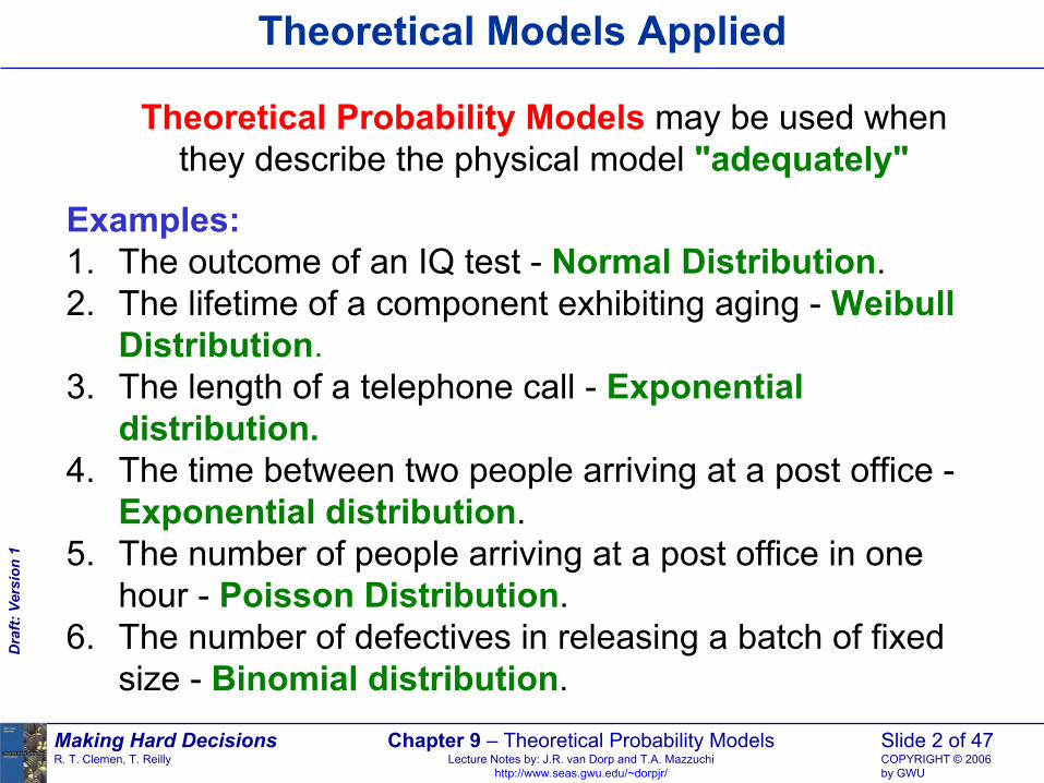
Theoretical Models Applied
Theoretical Probability Models may be used when they describe the physical model "adequately"
Examples:1. The outcome of an IQ test - Normal Distribution.2. The lifetime of a component exhibiting aging - Weibull
Distribution.3. The length of a telephone call - Exponential
distribution.4. The time between two people arriving at a post office -
Exponential distribution.5. The number of people arriving at a post office in one
hour - Poisson Distribution.6. The number of defectives in releasing a batch of fixed
size - Binomial distribution.

Making Hard DecisionsR. T. Clemen, T. Reilly
Chapter 9 – Theoretical Probability ModelsLecture Notes by: J.R. van Dorp and T.A. Mazzuchi
http://www.seas.gwu.edu/~dorpjr/
Slide 3 of 47COPYRIGHT © 2006by GWU
Dra
ft: V
ersi
on 1
The Binomial Distribution
Assumptions:1. A fixed number of trials, say N.2. Each trial results in a “Success” or “Failure”3. Each Trial has the same probability of success p.4. Different Trials are independent.
Define:X = “# Successes in a sequence of N trials”,
( , )X B N p ⇔∼
( , ) Pr( | , ) (1 ) ,x N xNX B N p X x N p p p
x−
⇔ = = ⋅ −
∼
0,1, ,x N=

Making Hard DecisionsR. T. Clemen, T. Reilly
Chapter 9 – Theoretical Probability ModelsLecture Notes by: J.R. van Dorp and T.A. Mazzuchi
http://www.seas.gwu.edu/~dorpjr/
Slide 4 of 47COPYRIGHT © 2006by GWU
Dra
ft: V
ersi
on 1
The Binomial Distribution
)!(!!xNx
NxN
−⋅=
! ( 1) ( 2) ( 3) 4 3 2 1N N N N N= ⋅ − ⋅ − ⋅ − ⋅ ⋅ ⋅
:Nx
• # of ways you can choose x from a group of N
• E[X] = N*p
• Var(X) = N*p*(1-p)

Making Hard DecisionsR. T. Clemen, T. Reilly
Chapter 9 – Theoretical Probability ModelsLecture Notes by: J.R. van Dorp and T.A. Mazzuchi
http://www.seas.gwu.edu/~dorpjr/
Slide 5 of 47COPYRIGHT © 2006by GWU
Dra
ft: V
ersi
on 1
The Binomial Distribution
DUAL RANDOM VARIABLE OF X:
X = “# Successes in a sequence of N trials”,
Y = “# Failures in a sequence of N trials”,
Y = N-X
Pr( | ,1 ) Pr( | , ) Pr( | , )Y y N p N X y N p X N y N p= − = − = = = −
yNyyNNyN ppyN
ppyN
N −−−− ⋅−
=−⋅
−
= )1()1( )(

Making Hard DecisionsR. T. Clemen, T. Reilly
Chapter 9 – Theoretical Probability ModelsLecture Notes by: J.R. van Dorp and T.A. Mazzuchi
http://www.seas.gwu.edu/~dorpjr/
Slide 6 of 47COPYRIGHT © 2006by GWU
Dra
ft: V
ersi
on 1
The Binomial Distribution
Conclusion:X ~ B(N,p) ⇔ Y ~ B(N,1-p)
Pretzel Example:You are planning to sell a new pretzel and you want to know whether it will be a success or not. Initially, you are 50% certain that it will be a “Hit”. Thus,
Pr(“Hit”) = Pr(“Flop”) = 0.5
If your pretzel is a “HIT” you expect to gain 30% of the market. Let X be the number of people out of a group of N that buy your pretzel.
Making Hard DecisionsR. T. Clemen, T. Reilly
Chapter 9 – Theoretical Probability ModelsLecture Notes by: J.R. van Dorp and T.A. Mazzuchi
http://www.seas.gwu.edu/~dorpjr/
Slide 7 of 47COPYRIGHT © 2006by GWU
Dra
ft: V
ersi
on 1
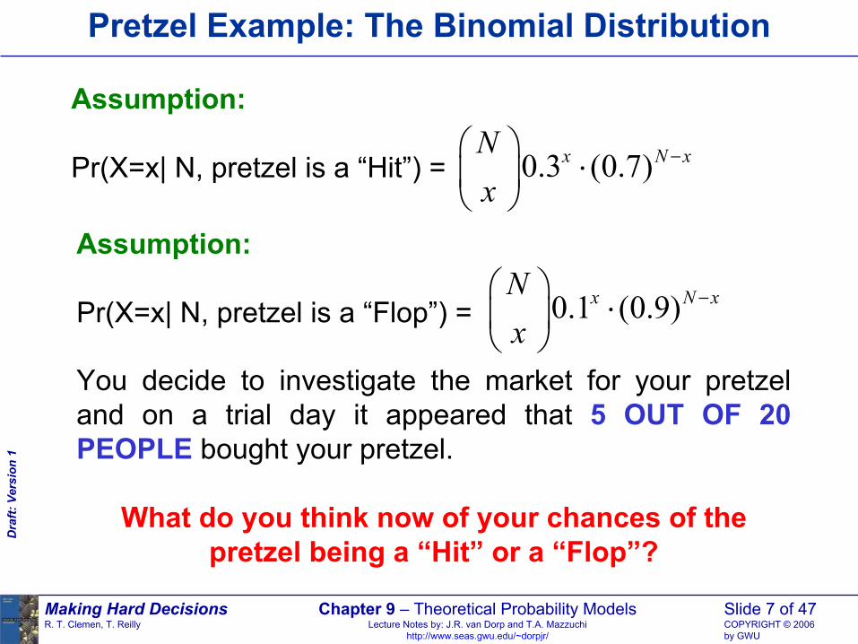
Pretzel Example: The Binomial Distribution
Assumption:
Pr(X=x| N, pretzel is a “Hit”) = 0.3 (0.7)x N xNx
− ⋅
Assumption:
Pr(X=x| N, pretzel is a “Flop”) = 0.1 (0.9)x N xNx
− ⋅
You decide to investigate the market for your pretzel and on a trial day it appeared that 5 OUT OF 20 PEOPLE bought your pretzel.
What do you think now of your chances of the pretzel being a “Hit” or a “Flop”?

Making Hard DecisionsR. T. Clemen, T. Reilly
Chapter 9 – Theoretical Probability ModelsLecture Notes by: J.R. van Dorp and T.A. Mazzuchi
http://www.seas.gwu.edu/~dorpjr/
Slide 8 of 47COPYRIGHT © 2006by GWU
Dra
ft: V
ersi
on 1
Pretzel Example: The Binomial Distribution
Notation: Data = (20,5)
Calculation:Pr(" " | )Hit Data =
Pr( | " ") Pr(" ")Pr( | " ") Pr(" ") Pr( | " ") Pr(" ")
Data Hit HitData Hit Hit Data Flop Flop+
179.0)7.0(3.0520
)"|"Pr( 155 =⋅
=HitData
(Table - Page 686)

Making Hard DecisionsR. T. Clemen, T. Reilly
Chapter 9 – Theoretical Probability ModelsLecture Notes by: J.R. van Dorp and T.A. Mazzuchi
http://www.seas.gwu.edu/~dorpjr/
Slide 9 of 47COPYRIGHT © 2006by GWU
Dra
ft: V
ersi
on 1
Pretzel Example: The Binomial Distribution
Conclusion:
848.05.0032.05.0179.0
5.0179.0)|"Pr(" =⋅+⋅
⋅=DataHit
Further Development of selling Pretzel may be warranted!
032.0)9.0(1.0520
)"|"Pr( 155 =⋅
=FlopData
(Table - Page 686)

Making Hard DecisionsR. T. Clemen, T. Reilly
Chapter 9 – Theoretical Probability ModelsLecture Notes by: J.R. van Dorp and T.A. Mazzuchi
http://www.seas.gwu.edu/~dorpjr/
Slide 10 of 47COPYRIGHT © 2006by GWU
Dra
ft: V
ersi
on 1
The Poisson Process and Distribution
Consider a particular event e.g. a customer arriving at a bank.
Assumptions:
1. The events can occur at any point in time.
2. The arrival rate per hour is constant, e.g. customers per hour.
3. The number of customers arriving in disjoint time intervals are independent of each other, e.g. the number of customers in the first hour day and the number of customers in the second hour of the day.
X(t) = ”# of such events in the time interval [0,t]”Define:

Making Hard DecisionsR. T. Clemen, T. Reilly
Chapter 9 – Theoretical Probability ModelsLecture Notes by: J.R. van Dorp and T.A. Mazzuchi
http://www.seas.gwu.edu/~dorpjr/
Slide 11 of 47COPYRIGHT © 2006by GWU
Dra
ft: V
ersi
on 1
The Poisson Process and Distribution
tmk
ektmtmkX ⋅−⋅==!)()),0[,|Pr(
Pr( | )!
knnY k n e
k−= = ⋅
•X(t) ~ Poisson(m*t):
• is called the Poisson distribution
• E[Y] = n
• Var[Y] = n
• E[X] =m*t
• Var[X]= m*t
Making Hard DecisionsR. T. Clemen, T. Reilly
Chapter 9 – Theoretical Probability ModelsLecture Notes by: J.R. van Dorp and T.A. Mazzuchi
http://www.seas.gwu.edu/~dorpjr/
Slide 12 of 47COPYRIGHT © 2006by GWU
Dra
ft: V
ersi
on 1
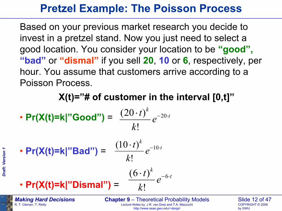
• Pr(X(t)=k|”Good”) =
• Pr(X(t)=k|”Bad”) =
• Pr(X(t)=k|”Dismal”) =
Pretzel Example: The Poisson ProcessBased on your previous market research you decide to invest in a pretzel stand. Now you just need to select a good location. You consider your location to be “good”,“bad” or “dismal” if you sell 20, 10 or 6, respectively, per hour. You assume that customers arrive according to a Poisson Process.
tk
ekt ⋅−⋅ 20
!)20(
tk
ekt ⋅−⋅ 10
!)10(
tk
ekt ⋅−⋅ 6
!)6(
X(t)=”# of customer in the interval [0,t]”

Making Hard DecisionsR. T. Clemen, T. Reilly
Chapter 9 – Theoretical Probability ModelsLecture Notes by: J.R. van Dorp and T.A. Mazzuchi
http://www.seas.gwu.edu/~dorpjr/
Slide 13 of 47COPYRIGHT © 2006by GWU
Dra
ft: V
ersi
on 1
Pretzel Example: The Poisson Process
Pr(“GOOD”) = 0.70, Pr(“BAD”) = 0.20, Pr(“DISMAL”) = 0.10
You give yourself one week for people to get to know you at this location. The second week, you open your stand in the morning and in the first half hour, 7 people bought your pretzel. Hmmm, You want to reevaluate your location.
SHOULD YOU RELOCATE?
Notation: Data = (7, [0,0.5))
We want to know:
?)|"Pr(" =DataGood

Making Hard DecisionsR. T. Clemen, T. Reilly
Chapter 9 – Theoretical Probability ModelsLecture Notes by: J.R. van Dorp and T.A. Mazzuchi
http://www.seas.gwu.edu/~dorpjr/
Slide 14 of 47COPYRIGHT © 2006by GWU
Dra
ft: V
ersi
on 1
• Pr(Data|”Good”)=Pr(X(0.5)=7|”Good”) =
= 0.09, Table – Page 700.• Pr(Data|”Bad”)=Pr(X(0.5)=7|”Bad”) =
= 0.104, Table – Page 698.• Pr(Data|”Dismal”)=Pr(X(0.5)=7|”Dismal”) =
= 0.022, Table – Page 698.
Pretzel Example: The Poisson Process
Calculation: =)|"Pr(" DataGoodPr( | " ") Pr(" ")
Pr( | " ") Pr(" ") Pr( | " ") Pr(" ") Pr( | " ") Pr(" ")Data Good Good
Data Good Good Data Bad Bad Data Dismal Dismal+ +
720 0.5(20 0.5)
7!e− ⋅⋅
710 0.5(10 0.5)
7!e− ⋅⋅
76 0.5(6 0.5)
7!e− ⋅⋅

Making Hard DecisionsR. T. Clemen, T. Reilly
Chapter 9 – Theoretical Probability ModelsLecture Notes by: J.R. van Dorp and T.A. Mazzuchi
http://www.seas.gwu.edu/~dorpjr/
Slide 15 of 47COPYRIGHT © 2006by GWU
Dra
ft: V
ersi
on 1
Pretzel Example: The Poisson Process
• Pr(“Good”) = 0.70, Pr(“Bad”) = 0.20, Pr(“Dismal”) = 0.10
733.010.0022.020.0104.070.009.0
70.009.0)|"Pr(" =⋅+⋅+⋅
⋅=DataGood
• Simlarly: Pr(‘Bad”|Data) = 0.242, Pr(“Dismal|Data) = 0.025
Conclusion:In light of the new data, you decide that the chances of this being a “Dismal” location for the pretzel stand is remote and your chance for this being a “Good” location has slightly improved. You decide to stay.

Making Hard DecisionsR. T. Clemen, T. Reilly
Chapter 9 – Theoretical Probability ModelsLecture Notes by: J.R. van Dorp and T.A. Mazzuchi
http://www.seas.gwu.edu/~dorpjr/
Slide 16 of 47COPYRIGHT © 2006by GWU
Dra
ft: V
ersi
on 1
The Exponential Distribution
Consider a particular event e.g. a customer arriving at a bank. Now consider, the length of time between two consecutive events e.g. the time between two customers arriving.
Alternative assumptions for Poisson process:1. The arrival rate per hour is constant, e.g. m customers
per hour.2. Inter-arrival Times are exponentially distributed with
parameter m.3. Customers arrive independently from each other.
Define:
T = “Time between two consecutive customers arriving”

Making Hard DecisionsR. T. Clemen, T. Reilly
Chapter 9 – Theoretical Probability ModelsLecture Notes by: J.R. van Dorp and T.A. Mazzuchi
http://www.seas.gwu.edu/~dorpjr/
Slide 17 of 47COPYRIGHT © 2006by GWU
Dra
ft: V
ersi
on 1
The Exponential Distribution
• T ~ Exponential(m):tm
T emtTmtF ⋅−−=≤= 1)|Pr()|(
• Cumulative Distribution Function of T (CDF):)|( mtFT
• The density function follows from
tmTT em
dtmtdFmtf ⋅−⋅== )|()|(

Making Hard DecisionsR. T. Clemen, T. Reilly
Chapter 9 – Theoretical Probability ModelsLecture Notes by: J.R. van Dorp and T.A. Mazzuchi
http://www.seas.gwu.edu/~dorpjr/
Slide 18 of 47COPYRIGHT © 2006by GWU
Dra
ft: V
ersi
on 1
The Exponential Distribution
Probability Density Function - Exp(2)
0
0.5
1
1.5
2
2.5
0.00 0.50 1.00 1.50 2.00 2.50 3.00 3.50 4.00
t
)2|(tfT
a

Making Hard DecisionsR. T. Clemen, T. Reilly
Chapter 9 – Theoretical Probability ModelsLecture Notes by: J.R. van Dorp and T.A. Mazzuchi
http://www.seas.gwu.edu/~dorpjr/
Slide 19 of 47COPYRIGHT © 2006by GWU
Dra
ft: V
ersi
on 1
The Exponential Distribution
amemaT ⋅−−=≤ 1)|Pr(•
• amemaTmaT ⋅−=≤−=> )|Pr(1)|Pr(
• =≤−≤=≤< )|Pr()|Pr()|Pr( mbTmaTmaTbambmbmam eeee ⋅−⋅−⋅−⋅− −=−−− )1(1
• 2
1 1[ ] , ( )E T Var Tm m
= =
Making Hard DecisionsR. T. Clemen, T. Reilly
Chapter 9 – Theoretical Probability ModelsLecture Notes by: J.R. van Dorp and T.A. Mazzuchi
http://www.seas.gwu.edu/~dorpjr/
Slide 20 of 47COPYRIGHT © 2006by GWU
Dra
ft: V
ersi
on 1
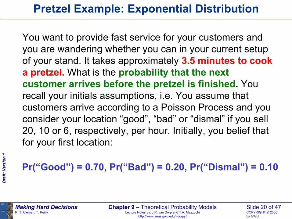
Pretzel Example: Exponential Distribution
You want to provide fast service for your customers and you are wandering whether you can in your current setup of your stand. It takes approximately 3.5 minutes to cook a pretzel. What is the probability that the next customer arrives before the pretzel is finished. You recall your initials assumptions, i.e. You assume that customers arrive according to a Poisson Process and you consider your location “good”, “bad” or “dismal” if you sell 20, 10 or 6, respectively, per hour. Initially, you belief that for your first location:
Pr(“Good”) = 0.70, Pr(“Bad”) = 0.20, Pr(“Dismal”) = 0.10

Making Hard DecisionsR. T. Clemen, T. Reilly
Chapter 9 – Theoretical Probability ModelsLecture Notes by: J.R. van Dorp and T.A. Mazzuchi
http://www.seas.gwu.edu/~dorpjr/
Slide 21 of 47COPYRIGHT © 2006by GWU
Dra
ft: V
ersi
on 1
Pretzel Example: Exponential Distribution
Calculation:+⋅>=> )"Pr(")"|"5.3Pr()5.3Pr( GoodGoodMinTMinT
+⋅> )"Pr(")"|"5.3Pr( BadBadMinT)"Pr(")"|"5.3Pr( DismalDismalMinT ⋅>
3.5Pr( 3.5 | " ") Pr( | 20)60
T Min Good T hours> = > =20 0.0583Pr( 0.0583 | 20) 0.3114T e− ⋅> = =
3.5Pr( 3.5 | " ") Pr( |10)60
T Min Bad T hours> = > =10 0.0583Pr( 0.0583 |10) 0.5580T e− ⋅> = =

Making Hard DecisionsR. T. Clemen, T. Reilly
Chapter 9 – Theoretical Probability ModelsLecture Notes by: J.R. van Dorp and T.A. Mazzuchi
http://www.seas.gwu.edu/~dorpjr/
Slide 22 of 47COPYRIGHT © 2006by GWU
Dra
ft: V
ersi
on 1
Pretzel Example: Exponential Distribution
3.5Pr( 3.5 | " ") Pr( | 6)60
T Min Dismal T hours> = > =6 0.0583Pr( 0.0583 | 6) 0.7047T e− ⋅> = =
Pr(“Good”) = 0.70, Pr(“Bad”) = 0.20, Pr(“Dismal”) = 0.10
Pr( 3.5 ) 0.3114 0.7 0.5580 0.2T Min> = ⋅ + ⋅0.7047 0.1 0.40+ ⋅ =
Or in other words: Pr( 3.5 ) 0.60T Min≤ =Conclusion:
60% of your customers will have to waituntil the pretzel is ready.
Making Hard DecisionsR. T. Clemen, T. Reilly
Chapter 9 – Theoretical Probability ModelsLecture Notes by: J.R. van Dorp and T.A. Mazzuchi
http://www.seas.gwu.edu/~dorpjr/
Slide 23 of 47COPYRIGHT © 2006by GWU
Dra
ft: V
ersi
on 1
Pretzel Example: Exponential Distribution
You realize that customers prefer hot pretzels and you are not to concerned about this number. However you decide to reevaluate after one week of operation. The second week, you open your stand in the morning and in the first half an hour 7 people brought your pretzel. What do you think now of is the percentage of people waiting for a pretzel.
Notation: Data = (7, [0,0.5))

Making Hard DecisionsR. T. Clemen, T. Reilly
Chapter 9 – Theoretical Probability ModelsLecture Notes by: J.R. van Dorp and T.A. Mazzuchi
http://www.seas.gwu.edu/~dorpjr/
Slide 24 of 47COPYRIGHT © 2006by GWU
Dra
ft: V
ersi
on 1
Pretzel Example: Exponential Distribution
=> )|5.3Pr( DataMinT+⋅> )|"Pr("),"|"5.3Pr( DataGoodDataGoodMinT
+⋅> )|"Pr("),"|"5.3Pr( DataBadDataBadMinT)|"Pr("),"|"5.3Pr( DataDismalDataDismalMinT ⋅>
Pr( 3.5 | " ", )T Min Good Data> =
Pr( 3.5 | " ", )T Min Bad Data> =
Pr( 3.5 | " ", )T Min Dismal Data> =
Pr( 3.5 | " ") 0.3114T Min Good> =
Pr( 3.5 | " ") 0.5580T Min Bad> =
Pr( 3.5 | " ") 0.7047T Min Dismal> =

Making Hard DecisionsR. T. Clemen, T. Reilly
Chapter 9 – Theoretical Probability ModelsLecture Notes by: J.R. van Dorp and T.A. Mazzuchi
http://www.seas.gwu.edu/~dorpjr/
Slide 25 of 47COPYRIGHT © 2006by GWU
Dra
ft: V
ersi
on 1
Pretzel Example: Exponential Distribution
733.0)|"Pr(" =DataGood 242.0)|"Pr(" =DataBad025.0)|"Pr(" =DataDismal
Hence:Pr( 3.5 | )T Min Data> =
3809.0025.07047.0242.05580.0733.03114.0 =⋅+⋅+⋅
Or in other words: 62.0)|5.3Pr( =≤ DataMinTConclusion:
62% of your customers will have to wait until the pretzel is ready (which increased from the previous 60%. You are concerned about the chance of customers waiting increasing. You decide to continue to monitor this percentage and may consider investing in another pretzel oven.
Making Hard DecisionsR. T. Clemen, T. Reilly
Chapter 9 – Theoretical Probability ModelsLecture Notes by: J.R. van Dorp and T.A. Mazzuchi
http://www.seas.gwu.edu/~dorpjr/
Slide 26 of 47COPYRIGHT © 2006by GWU
Dra
ft: V
ersi
on 1
The Normal Distribution
•
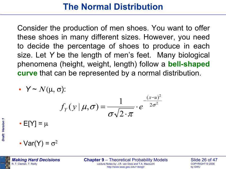
Consider the production of men shoes. You want to offer these shoes in many different sizes. However, you need to decide the percentage of shoes to produce in each size. Let Y be the length of men’s feet. Many biological phenomena (height, weight, length) follow a bell-shaped curve that can be represented by a normal distribution.
Y ~ Ν (µ, σ):
2
2
2)(
21),|( σ
πσσµ
ux
Y eyf−−
⋅⋅
=
• E[Y] = µ
• Var(Y) = σ2

Making Hard DecisionsR. T. Clemen, T. Reilly
Chapter 9 – Theoretical Probability ModelsLecture Notes by: J.R. van Dorp and T.A. Mazzuchi
http://www.seas.gwu.edu/~dorpjr/
Slide 27 of 47COPYRIGHT © 2006by GWU
Dra
ft: V
ersi
on 1
The Normal Distribution
• Some handy rules of thumb:
68.0)Pr( ≈+<<− σµσµ Y
95.0)22Pr( ≈+<<− σµσµ Y
99.0)33Pr( ≈+<<− σµσµ Y

Making Hard DecisionsR. T. Clemen, T. Reilly
Chapter 9 – Theoretical Probability ModelsLecture Notes by: J.R. van Dorp and T.A. Mazzuchi
http://www.seas.gwu.edu/~dorpjr/
Slide 28 of 47COPYRIGHT © 2006by GWU
Dra
ft: V
ersi
on 1
The Normal Distribution
Probability Density Function - N(2,0.5)
00.10.20.30.40.50.60.70.80.9
0.00 0.50 1.00 1.50 2.00 2.50 3.00 3.50 4.00
≈ 68%≈ 95%≈ 99%

Making Hard DecisionsR. T. Clemen, T. Reilly
Chapter 9 – Theoretical Probability ModelsLecture Notes by: J.R. van Dorp and T.A. Mazzuchi
http://www.seas.gwu.edu/~dorpjr/
Slide 29 of 47COPYRIGHT © 2006by GWU
Dra
ft: V
ersi
on 1
The Normal Distribution
Define:
σµ−= YZ
• Z Standard Normal Distributed ⇔ Z ~ N(0,1)
• The Standard Normal CDF is available in Table Format.
• Normal distribution is symmetric around its mean:
⇔>−=−<− ),|Pr(),|Pr( σµµσµµ yYyY
)Pr()Pr( zZzZ >=−<

Making Hard DecisionsR. T. Clemen, T. Reilly
Chapter 9 – Theoretical Probability ModelsLecture Notes by: J.R. van Dorp and T.A. Mazzuchi
http://www.seas.gwu.edu/~dorpjr/
Slide 30 of 47COPYRIGHT © 2006by GWU
Dra
ft: V
ersi
on 1
How do we calculate if only the CDF for Z is available in Table format?
The Normal Distribution
),|Pr( σµbYa ≤<
Convert to a Standard Normal Distribution:
=−≤−<−=≤< ),|Pr(),|Pr( σµσ
µσ
µσ
µσµ bYabYa
)Pr()Pr()Pr(σ
µσ
µσ
µσ
µ −≤−−≤=−≤<− aZbZbZa
Making Hard DecisionsR. T. Clemen, T. Reilly
Chapter 9 – Theoretical Probability ModelsLecture Notes by: J.R. van Dorp and T.A. Mazzuchi
http://www.seas.gwu.edu/~dorpjr/
Slide 31 of 47COPYRIGHT © 2006by GWU
Dra
ft: V
ersi
on 1
The Normal Distribution
Example: Probability Density Function - N(2,0.5)
00.10.20.30.40.50.60.70.80.9
0.00 0.50 1.00 1.50 2.00 2.50 3.00 3.50 4.00
?
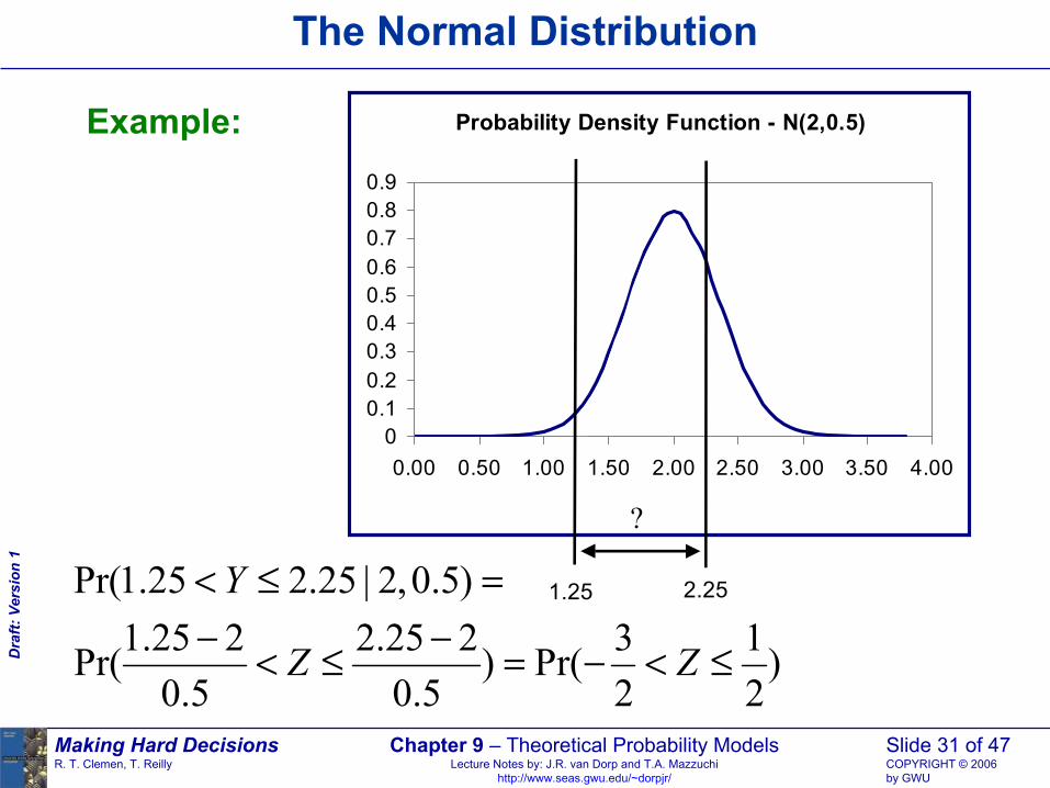
1.25 2.25Pr(1.25 2.25 | 2,0.5)Y< ≤ =1.25 2 2.25 2 3 1Pr( ) Pr( )
0.5 0.5 2 2Z Z− −< ≤ = − < ≤

Making Hard DecisionsR. T. Clemen, T. Reilly
Chapter 9 – Theoretical Probability ModelsLecture Notes by: J.R. van Dorp and T.A. Mazzuchi
http://www.seas.gwu.edu/~dorpjr/
Slide 32 of 47COPYRIGHT © 2006by GWU
Dra
ft: V
ersi
on 1
The Normal Distribution
Probability Density Function - N(0,1)
-2.50 -2.00 -1.50 -1.00 -0.50 0.00 0.50 1.00 1.50 2.00
50.15.0
225.1 −≈− 50.05.0
225.2 ≈−
Making Hard DecisionsR. T. Clemen, T. Reilly
Chapter 9 – Theoretical Probability ModelsLecture Notes by: J.R. van Dorp and T.A. Mazzuchi
http://www.seas.gwu.edu/~dorpjr/
Slide 33 of 47COPYRIGHT © 2006by GWU
Dra
ft: V
ersi
on 1
The Normal Distribution
Probability Density Function - N(0,1)
-2.50 -2.00 -1.50 -1.00 -0.50 0.00 0.50 1.00 1.50 2.00
50.05.0
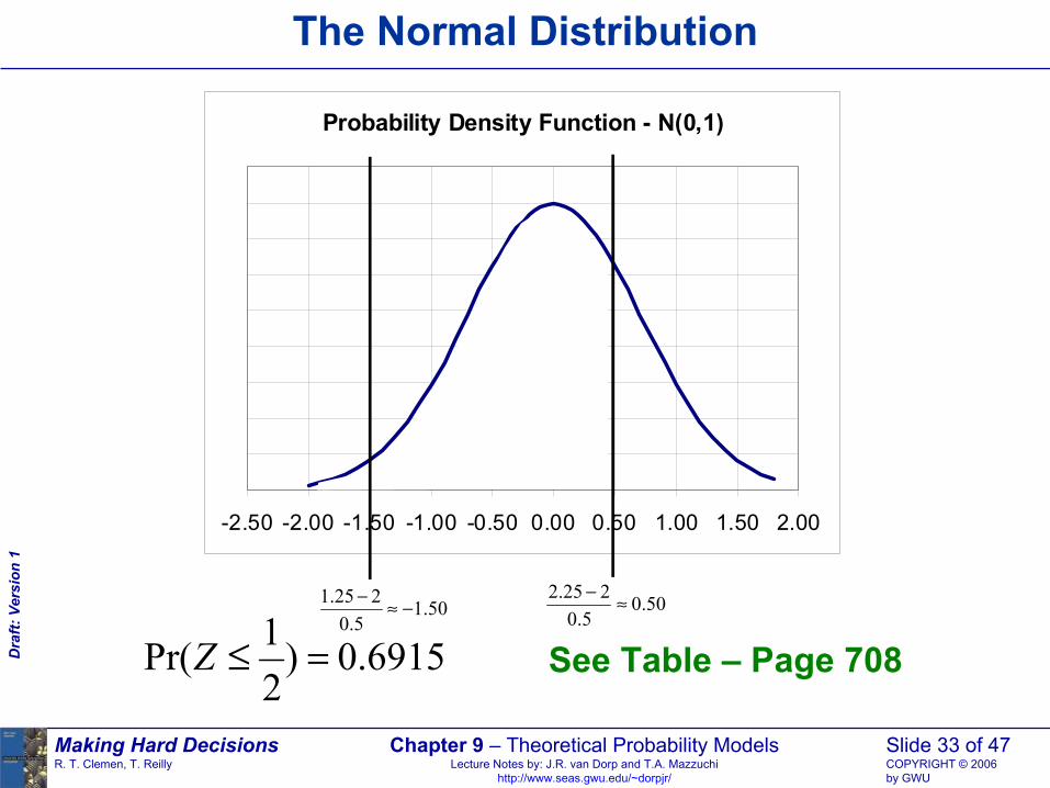
225.2 ≈−50.1
5.0225.1 −≈−
1Pr( ) 0.69152
Z ≤ = See Table – Page 708
Making Hard DecisionsR. T. Clemen, T. Reilly
Chapter 9 – Theoretical Probability ModelsLecture Notes by: J.R. van Dorp and T.A. Mazzuchi
http://www.seas.gwu.edu/~dorpjr/
Slide 34 of 47COPYRIGHT © 2006by GWU
Dra
ft: V
ersi
on 1
The Normal Distribution
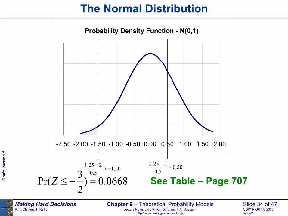
3Pr( ) 0.06682
Z ≤ − = See Table – Page 707
Probability Density Function - N(0,1)
-2.50 -2.00 -1.50 -1.00 -0.50 0.00 0.50 1.00 1.50 2.00
50.05.0
225.2 ≈−50.1
5.0225.1 −≈−
Making Hard DecisionsR. T. Clemen, T. Reilly
Chapter 9 – Theoretical Probability ModelsLecture Notes by: J.R. van Dorp and T.A. Mazzuchi
http://www.seas.gwu.edu/~dorpjr/
Slide 35 of 47COPYRIGHT © 2006by GWU
Dra
ft: V
ersi
on 1
The Normal Distribution
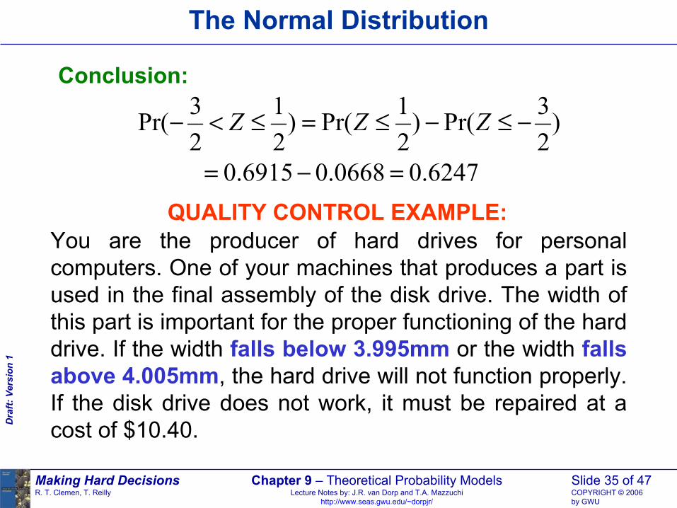
Conclusion:
)23Pr()
21Pr()
21
23Pr( −≤−≤=≤<− ZZZ
6247.00668.06915.0 =−=QUALITY CONTROL EXAMPLE:
You are the producer of hard drives for personal computers. One of your machines that produces a part is used in the final assembly of the disk drive. The width of this part is important for the proper functioning of the hard drive. If the width falls below 3.995mm or the width falls above 4.005mm, the hard drive will not function properly. If the disk drive does not work, it must be repaired at a cost of $10.40.

Making Hard DecisionsR. T. Clemen, T. Reilly
Chapter 9 – Theoretical Probability ModelsLecture Notes by: J.R. van Dorp and T.A. Mazzuchi
http://www.seas.gwu.edu/~dorpjr/
Slide 36 of 47COPYRIGHT © 2006by GWU
Dra
ft: V
ersi
on 1
QC Example: The Normal Distribution
The machine can be set a width of 4mm, but it is not perfectly accurate. The production speed of the machine can be set high or low. However, the higher production speed result in lower accuracy. In fact, if W is the width of the part:
(W| High Production Speed) ~ N(4, 0.0026)(W| Low Production Speed) ~ N(4, 0.0019)
Of course at a higher production speed more hard drives are produced and the cost per hard drive is $20.45. At the lower production speed the cost per hard drive is $20.75.
Should you turn at high production speedor low production speed?

Making Hard DecisionsR. T. Clemen, T. Reilly
Chapter 9 – Theoretical Probability ModelsLecture Notes by: J.R. van Dorp and T.A. Mazzuchi
http://www.seas.gwu.edu/~dorpjr/
Slide 37 of 47COPYRIGHT © 2006by GWU
Dra
ft: V
ersi
on 1
QC Example: The Normal Distribution
Calculation: Production At Low Speed
Pr(Defective| Low Speed) = 1 Pr(Not Defective| Low Speed)−
1 Pr(3.995 4.005 | 4, 0.0019)W µ σ= − < ≤ = = =
)0019.0,4|0019.0
4005.40019.0
40019.0
4995.3Pr(1 ==−≤−<−− σµW
( ))63.2Pr()63.2Pr(1)63.263.2Pr(1 −≤−≤−=≤<−−= ZZZ
1 (0.9957 0.0043) 1 0.9914 0.0086− − = − =
See Table – Page 709,707

Making Hard DecisionsR. T. Clemen, T. Reilly
Chapter 9 – Theoretical Probability ModelsLecture Notes by: J.R. van Dorp and T.A. Mazzuchi
http://www.seas.gwu.edu/~dorpjr/
Slide 38 of 47COPYRIGHT © 2006by GWU
Dra
ft: V
ersi
on 1
QC Example: The Normal Distribution
Calculation: Production at High Speed
Pr(Defective| High Speed) = 1 Pr(Not Defective| High Speed)−
1 Pr(3.995 4.005 | 4, 0.0026)W µ σ= − < ≤ = = =
3.995 4 4 4.005 41 Pr( | 4, 0.0026)0.0026 0.0026 0.0026
W µ σ− − −− < ≤ = =
( )1 Pr( 1.92 1.92) 1 Pr( 1.92) Pr( 1.92)Z Z Z= − − < ≤ = − ≤ − ≤ −
1 (0.9726 0.0274) 1 0.9452 0.0548− − = − =
See Table – Page 709,707

Making Hard DecisionsR. T. Clemen, T. Reilly
Chapter 9 – Theoretical Probability ModelsLecture Notes by: J.R. van Dorp and T.A. Mazzuchi
http://www.seas.gwu.edu/~dorpjr/
Slide 39 of 47COPYRIGHT © 2006by GWU
Dra
ft: V
ersi
on 1
QC Example: The Normal Distribution
High Speed
Low Speed
Not Defective (0.9452)
Defective (0.0548)
Min Cost
$31.15
$20.45
Not Defective (0.9914)
Defective (0.0086)$10.40
$0
$10.40
$0
EMV=$20.84
EMV=$21.02
EMV=$20.84 $20.75
$30.85
$20.45
$20.75
Conclusion: Run at a slower speed. Increased cost from slow speedare offset by the increased precision.

Making Hard DecisionsR. T. Clemen, T. Reilly
Chapter 9 – Theoretical Probability ModelsLecture Notes by: J.R. van Dorp and T.A. Mazzuchi
http://www.seas.gwu.edu/~dorpjr/
Slide 40 of 47COPYRIGHT © 2006by GWU
Dra
ft: V
ersi
on 1
The Beta Distribution
Suppose you are interested in the proportion of voters in your town that will vote for the next republican president. This proportion is uncertain and may range from 0 to 1.
Let Q be that proportion and assume Q~Beta(n,p)
10,)1()()(
)(),|( 11 <<−⋅−Γ⋅Γ
Γ= −−− qqqrnr
nrnqf rnrQ
,...3,2,1,123)2()1()!1()( =⋅⋅⋅−⋅−=−=Γ nnnnn

Making Hard DecisionsR. T. Clemen, T. Reilly
Chapter 9 – Theoretical Probability ModelsLecture Notes by: J.R. van Dorp and T.A. Mazzuchi
http://www.seas.gwu.edu/~dorpjr/
Slide 41 of 47COPYRIGHT © 2006by GWU
Dra
ft: V
ersi
on 1
The Beta Distribution
0.00
0.50
1.00
1.50
2.00
2.50
3.00
3.50
4.00
0.00 0.20 0.40 0.60 0.80 1.00
q
),|( rnqfQ
n=20,r=10
n=8,r=4
n=4,r=2
n=2,r=1
SYMMETRIC BETA DISTRIBUTIONS
Making Hard DecisionsR. T. Clemen, T. Reilly
Chapter 9 – Theoretical Probability ModelsLecture Notes by: J.R. van Dorp and T.A. Mazzuchi
http://www.seas.gwu.edu/~dorpjr/
Slide 42 of 47COPYRIGHT © 2006by GWU
Dra
ft: V
ersi
on 1
The Beta Distribution
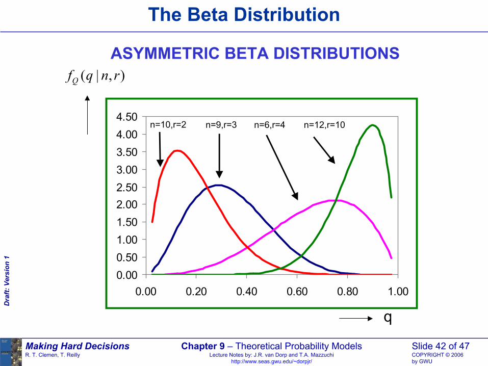
ASYMMETRIC BETA DISTRIBUTIONS
0.000.501.001.502.002.503.003.504.004.50
0.00 0.20 0.40 0.60 0.80 1.00
q
),|( rnqfQ
n=10,r=2 n=9,r=3 n=6,r=4 n=12,r=10

Making Hard DecisionsR. T. Clemen, T. Reilly
Chapter 9 – Theoretical Probability ModelsLecture Notes by: J.R. van Dorp and T.A. Mazzuchi
http://www.seas.gwu.edu/~dorpjr/
Slide 43 of 47COPYRIGHT © 2006by GWU
Dra
ft: V
ersi
on 1
The Beta Distribution
[ ] rE Qn
=2
( )( )( 1)r n rVar Qn n
−=+
Elicitation Of Parameters Using Informal Parameter Interpretation:
n = “Number of Trials”r = “Number of Successes”
EXAMPLE:You first guess for the preference of the Republican Candidate is that 4 out of 10 people would vote for the Republican Candidate. You set: n=10, r=4.
Note this coincides with an expected proportion of 40%.

Making Hard DecisionsR. T. Clemen, T. Reilly
Chapter 9 – Theoretical Probability ModelsLecture Notes by: J.R. van Dorp and T.A. Mazzuchi
http://www.seas.gwu.edu/~dorpjr/
Slide 44 of 47COPYRIGHT © 2006by GWU
Dra
ft: V
ersi
on 1
The Beta Distribution
After talking to people on the street you reevaluate your beliefs and estimate that 40 out of 100 people would vote for the Republican Candidate. You set: n = 100, r = 40. Note that this still also coincides with an expected proportion of 40%.
What is the difference with the previous estimate?
First Estimate:
2
4(10 4). .( ) 14.7%10 (10 1)
St Dev Q −= =+
Second Estimate:
2
40(100 40). .( ) 4.9%100 (100 1)
St Dev Q −= =+

Making Hard DecisionsR. T. Clemen, T. Reilly
Chapter 9 – Theoretical Probability ModelsLecture Notes by: J.R. van Dorp and T.A. Mazzuchi
http://www.seas.gwu.edu/~dorpjr/
Slide 45 of 47COPYRIGHT © 2006by GWU
Dra
ft: V
ersi
on 1
Pretzel Example: The Beta Distribution
You want to re evaluate your decision to invest in a pretzel stand. Sales have been okay in the first week, but not too great. You are wandering whether you should proceed. You estimate at this point that you are 50% sure that your market share is less than 20% and your 75% sure that your market share is less than 38%.
Let Q be the proportion of the market. You decide to model your uncertainty in Q as a beta distribution and using the table on page 711 that:
49.0)1,4|20.0Pr( ===≤ rnQ
76.0)1,4|38.0Pr( ===≤ rnQ

Making Hard DecisionsR. T. Clemen, T. Reilly
Chapter 9 – Theoretical Probability ModelsLecture Notes by: J.R. van Dorp and T.A. Mazzuchi
http://www.seas.gwu.edu/~dorpjr/
Slide 46 of 47COPYRIGHT © 2006by GWU
Dra
ft: V
ersi
on 1
Pretzel Example: The Beta Distribution
You decide that that is close enough and proceed with the analysis. You estimate that the total monthly market is 100,000 pretzels. Your price for a pretzel is set at $0.50 and it costs you $0.10 to produce a pretzel. You estimate $8000of monthy fixed cost for your pretzel stand and some overhead. Given the market share Q, you calculate for your net monthly profit:
Net Profit = Revenue – Cost100000*Q*$0.50 – (100000*Q*$0.10+8000)
= 40000*Q-8000
However, Q is uncertain so you decide to calculate your expected profit.
Making Hard DecisionsR. T. Clemen, T. Reilly
Chapter 9 – Theoretical Probability ModelsLecture Notes by: J.R. van Dorp and T.A. Mazzuchi
http://www.seas.gwu.edu/~dorpjr/
Slide 47 of 47COPYRIGHT © 2006by GWU
Dra
ft: V
ersi
on 1
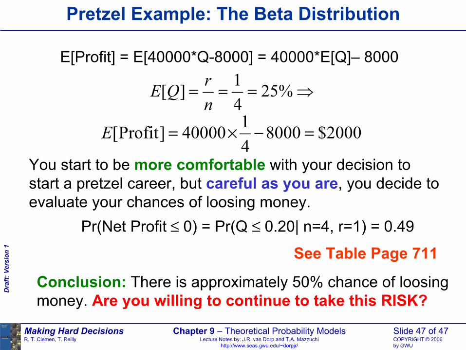
Pretzel Example: The Beta Distribution
E[Profit] = E[40000*Q-8000] = 40000*E[Q]– 80001[ ] 25%4
rE Qn
= = = ⇒
1[Profit] 40000 8000 $20004
E = × − =
You start to be more comfortable with your decision to start a pretzel career, but careful as you are, you decide to evaluate your chances of loosing money.
Pr(Net Profit ≤ 0) = Pr(Q ≤ 0.20| n=4, r=1) = 0.49
See Table Page 711
Conclusion: There is approximately 50% chance of loosing money. Are you willing to continue to take this RISK?