Chapter 9

Demand-Side Equilibrium:

Unemployment or Inflation?

A definite ratio, to be called the Multiplier, can be established

between income and investment.JOHN MAYNARD KEYNES

Outline

• Suppose AS is given, how does ADAD affect the equilibriumequilibrium?

The Meaning Of Equilibrium GDP

• Assumptions – Constant

• Government expenditure G• Price level • Rate of interest → I constant• International value of the dollar → X-IM

constant

• Total production (Y) = Total income (NI)• Total expenditure (AD) = C + I + G + (X-

IM)3

The circular flow diagram

Figure 1

4

The Meaning Of Equilibrium GDP

• Equilibrium– Consumers & firms

• No incentive to change behavior• Content - continue with things as they are

• If Total spending > Output– No equilibrium GDP

– Firms - Depleting inventory stocks• Increase production

– Meet higher demand

• Raise prices5

The Meaning Of Equilibrium GDP

• If Total spending < Output– No equilibrium GDP

– Firms• Inventory increase• Decrease production • Cut prices

– Stimulate demand

6

The Meaning Of Equilibrium GDP

• If Total Spending = Output– Equilibrium level of GDP - demand side

– Firms• Inventories - desired levels• No incentive to change

– Output– Prices

7

Mechanics of Income Determination

• Assumption– I, G, and X-IM are fixed

• Total expenditure = C + I + G +(X-IM)• Induced investment

– Part of investment spending• Rises - GDP rises• Falls - GDP falls

8

The total expenditure schedule

Table 1

9

(1) (2) (3) (4) (5) (6)

GDP(Y)

Consumption(C)

Investment(I)

Government Purchases (G)

Net Exports(X-IM)

Total Expenditure

4,8005,2005,6006,0006,4006,8007,200

3,0003,3003,6003,9004,2004,5004,800

900900900900900900900

1,3001,3001,3001,3001,3001,3001,300

-100-100-100-100-100-100-100

5,1005,4005,7006,0006,3006,6006,900

Construction of the expenditure schedule

Figure 2

10

Rea

l Exp

endi

ture

5,200 5,600 6,0000 6,400 6,800

Real GDP

7,200

3,900

4,800 C

6,0006,100

C+I

C+I+GC+I+G+(X-IM)

I=$900

G=$1,300

X-IM=-$100

Mechanics of Income Determination

• Expenditure schedule– Relationship

• National income (GDP)• Total spending

• Condition for equilibrium GDP (Y)

Y = C + I + G + (X-IM)

11

The determination of equilibrium output

Table 2

12

(1) (2) (3) (4) (5)

Output (Y)

Total Spending[C+I+G+(X-IM)]

Balance ofSpending & Output

InventoryStatus

Producer Response

4,8005,2005,6006,0006,4006,8007,200

5,1005,4005,7006,0006,3006,6006,900

Spending exceeds outputSpending exceeds outputSpending exceeds output

Spending = outputOutput exceeds spendingOutput exceeds spendingOutput exceeds spending

FallingFallingFalling

ConstantRisingRisingRising

Produce moreProduce moreProduce more

No changeProduce lessProduce lessProduce less

Mechanics of Income Determination

• Income-expenditure diagram– 45° line diagram

– Plots• Total real expenditure - vertical axis• Real income - horizontal axis

– Specific price level

• 45° line– Marks off points:

• Income = expenditure

13

Income-expenditure diagram

Figure 3

14

4,800 5,200 5,6000 6,000 6,400

Real GDP

6,800 7,200

4,800

5,200

5,600

6,000

6,400

Rea

l Exp

endi

ture

6,800

7,200

45°

C+I+G+(X-IM)

E

Equilibrium

Spending exceeds output

Output exceeds

spending

Mechanics of Income Determination

• If Expenditure line – above 45° line– Total spending > Total output

– Production – below equilibrium• Inventories – fall• Firms - increase production

• If Expenditure line- below 45° line– Total spending < Total output

– Production – above equilibrium• Inventories – rise• Firms - cut back production 15

Aggregate Demand Curve

• Higher prices– Decrease demand for goods & services

– Erode purchasing power• Of consumer wealth

– Lower real wealth

– Less spending• Any given level of real income

– Lower consumption function• Shift downward

16

Aggregate Demand Curve

• Lower prices– Increase demand for goods & services

– Enhance purchasing power• Of consumer wealth

– Higher real wealth

– More spending• Any given level of real income

– Higher consumption function• Shift upward

17

Shift of the consumption function

Figure 4

18

C0

Rea

l Con

sum

er S

pend

ing

Real Disposable Income

A

C2

C1Movements along

consumption function

Shifts of consumption

function

Aggregate Demand Curve

• Higher prices• Lower consumption function

– Total expenditure – shift downward

– Equilibrium quantity of real GDP demanded• Decreases

• Lower prices• Higher consumption function

– Total expenditure – shift upward

– Equilibrium quantity of real GDP demanded• Increases 19

Effect of the price level on equilibrium aggregate quantity demanded

Figure 5

20

Real GDP

Rea

l Exp

endi

ture

45°

45°

Y0

C0+I+G+(X-IM)E0

C1+I+G+(X-IM)

Y1

E1

(a) Rise in price level

Real GDP

Rea

l Exp

endi

ture

45°

45°

Y0

C0+I+G+(X-IM)E0

C2+I+G+(X-IM)

Y2

E2

(b) Fall in price level

The aggregate demand curve

Figure 6

21

Real GDP

Pric

e Le

vel

Y1 Y0 Y2

P2

P0

P1

E0

E2

E1

Demand-Side Equilibrium&Full Employment

• Potential GDP– Full-employment level of output

• Equilibrium GDP < potential GDP – Occurs:

• Low spending (consumers C↓, investors I↓)• Low government spending (G↓)• Weak foreign demand (X↓)• Price level - too high (X↓, IM↑)

22

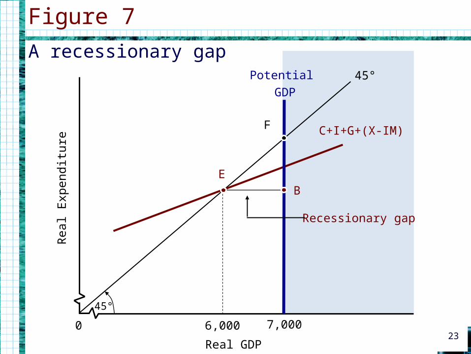
A recessionary gap

Figure 7

230

Real GDP

Rea

l Exp

endi

ture

45°

C+I+G+(X-IM)

6,000 7,000

Potential

GDP

F

B

E

Recessionary gap

45°

Demand-Side Equilibrium&Full Employment

• Equilibrium GDP < potential GDP – Unemployment & Recession

– RecessionaryRecessionary gap - amount• Equilibrium level of real GDP• Falls short of potential GDP

– To reach full employment• IncreaseIncrease total expenditure line

24

Demand-Side Equilibrium&Full Employment

• Equilibrium GDP > potential GDP– Occurs because

• High spending (consumer C↑, investment I↑)• Strong foreign demand (X↑)• Government spends too much (G↑)• Low price level (X↑, IM↓)

25

An inflationary gap

Figure 8

260

Real GDP

Rea

l Exp

endi

ture

45°

C+I+G+(X-IM)

8,0007,000

Potential

GDP

F

BE

Inflationary gap

45°

Demand-Side Equilibrium&Full Employment

• Equilibrium GDP > potential GDP– Inflation

– InflationaryInflationary gap• Equilibrium real GDP• Exceeds full-employment level of GDP

– To reach full employment• DecreaseDecrease total expenditure line

27

Demand-Side Equilibrium&Full Employment

• Full employment– Occurs:

• Spending plans – just right• Price level – just right

– No recessionary gap

– No inflationary gap

28

Coordination of Saving & Investment

• If S = I– Equilibrium at full employment

• On demand side• AD=C+I=GDP=NI=C+S → S=I

• If S ≠ I– Full employment is not an equilibrium

• S<I → inflationary gap• S>I → recessionary gap

29

A simplified circular flow

Figure 9

30

Coordination of Saving & Investment

• Unemployment– Total spending - too low

– Stems from coordination failure• Savers are different from Investors

• Coordination failure– Party A – want to change behavior, if

• Party B – changes

– No changes – no coordination

31

Changes on Demand Side: Multiplier Analysis

• Question: What’s the effect of changes in C, I, G, (X-IM) on Y?

• Multiplier – Ratio of Change in equilibrium GDP (Y) by original change in spending

• Multiplier principle– GDP – rises by moremore than

• Change in spending

• Multiplier > 1

32

Total expenditure after a $200 billion increase in investment spending

• Multiplier = ∆Y/ ∆I = 800/200 = 4

Table 3

33

(1) (2) (3) (4) (5) (6)

GDP(Y)

Consumption(C)

Investment(I)

Government Purchases (G)

Net Exports(X-IM)

Total Expenditure

4,8005,2005,6006,0006,4006,8007,200

3,0003,3003,6003,9004,2004,5004,800

1,1001,1001,1001,1001,1001,1001,100

1,3001,3001,3001,3001,3001,3001,300

-100-100-100-100-100-100-100

5,3005,6005,9006,2006,5006,8007,100

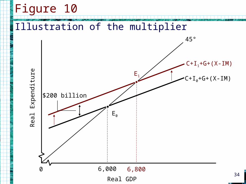
Illustration of the multiplier

Figure 10

340

Real GDP

Rea

l Exp

endi

ture

45°

C+I1+G+(X-IM)

6,8006,000

C+I0+G+(X-IM)

E0

E1

$200 billion

Multiplier Analysis

• Multiplier =

= 1 + MPC + (MPC)^2 + (MPC)^3 +…• Oversimplified multiplier formula

• Actual multiplier– Much lower

35

MPC11

Multiplier

The multiplier spending chain

Table 4

36

(1) (2) (3)

RoundNumber

Spending inThis Round

CumulativeTotal

123456789

10...20...

“Infinity”

$1,000,000750,000562,500421,875316,406237,305177,979133,484100,11375,085

…4,228

…0

$1,000,0001,750,0002,312,5002,734,3753,050,7813,288,0863,466,0653,599,5493,600,6223,774,747

..3,987,317

…4,000,000

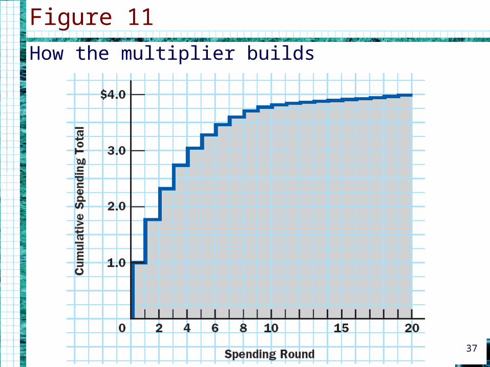
How the multiplier builds

Figure 11

37

Multiplier is a General Concept

• InducedInduced increase in consumption spending– From: increase in consumer incomes– Movement alongalong consumption function

• AutonomousAutonomous increase in consumption– Independently of consumer incomes– ShiftShift of consumption function

• Only autonomous increase brings multiplier effect

• Change in C, I, G, or (X-IM)– SameSame multiplier effect 38

Total expenditure after consumers decide to spend $200 billion more (Autonomous increase)

Table 5

39

(1) (2) (3) (4) (5) (6)

GDP(Y)

Consumption(C)

Investment(I)

Government Purchases (G)

Net Exports(X-IM)

Total Expenditure

4,8005,2005,6006,0006,4006,8007,200

3,2003,5003,8004,1004,4004,7005,000

900900900900900900900

1,3001,3001,3001,3001,3001,3001,300

-100-100-100-100-100-100-100

5,3005,6005,9006,2006,5006,8007,100

Multiplier is a General Concept

• GDPs of major economies– Linked by trade

• Boom in one country– Raise its imports

– Other countries• More exports• Increase GDP

• Recession in one country– Other countries

• Decrease GDP 40

Multiplier is a General Concept

• Booms and recessions tend to be transmittedtransmitted across national borders

Multiplier & Aggregate Demand Curve

• Income-expenditure diagrams– GivenGiven price level

• Different price levels– Different total expenditure curves

• Increase in spending– Given price level

– Multiplier effect

– Horizontal shift of aggregate demand

42

Multiplier & Aggregate Demand Curve

• An autonomous increase in spending leads to a horizontal shifthorizontal shift of the AD curve by an amount given by the oversimplified multiplier formula.

Two view of the multiplier

Figure 12

44

0 Real GDP

Rea

l Exp

endi

ture

45° C+I1+G+(X-IM)

6,8006,000

C+I0+G+(X-IM)

E0

E1$200 billion

0 Real GDP

Pric

e Le

vel

6,8006,000

D0

D0 (I=$900)

D1

D1 (I=$1,100)

E1

100E0

Summary

• Demand side equilibrium

Y = AD = C + I +G +(X-IM)• Income-expenditure diagram• Derivation of AD curve• Inflationary gap vs. Recessionary gap• Multiplier is same for an autonomous

increase in C, I, G, and (X-IM)• Multiplier = 1/(1-MPC)

APPENDIX A

Algebra of income determination & multiplier

• b = MPC

46

bIM)(XGIbTa

Y

bDIaC

TYDI

IMXGICY

1

)(

b-11

Yin Change

APPENDIX B

Multiplier with variable imports• Our GDP – increase

– Our imports – increase

• Our exports– Relatively insensitive to own GDP

– Sensitive – other countries GDP

• International trade– Lowers – value of multiplier

47

Equilibrium income with variable imports

Table 6

48

(1) (2) (3) (4) (5) (6) (7) (8)

GrossDomesticProduct

(Y)

ConsumerExpenditures

(C)Investment

(I)Government Purchases (G)

Exports(X)

Imports (IM)

NetExports(X-IM)

Total Expenditure

[C+I+G+(X-IM)]

4,8005,2005,6006,0006,4006,8007,200

3,0003,3003,6003,9004,2004,5004,800

900900900900900900900

1,3001,3001,3001,3001,3001,3001,300

650650650650650650650

570630690750810870930

+80+20-40

-100-160-220-280

5,2805,5205,7606,0006,2406,4806,720

The dependence of net exports on GDP

Figure 13

49

4,800 5,200 5,6000 6,000 6,400 Real GDP6,800 7,200

450550650750850

Rea

l Exp

orts

& I

mpo

rts

950IM

X

Negative net exportsPositive net exports

4,800 5,200 5,6006,000

6,400

Real GDP

6,800 7,200

-300-200-100

0100

Rea

l Net

Exp

orts 200

X-IM

Negative net exportsPositive net exports

APPENDIX B

Multiplier with variable imports• Our GDP – increase

– Net exports – decline

• International trade– Lowers – value of multiplier

• Any autonomous increase in spending– Partly dissipated

• Purchases of foreign goods

– Additional income – foreigners

50

Equilibrium GDP with variable imports

Figure 14

51

0 Real GDP

Rea

l Exp

endi

ture

45°

C+I+G+(X-IM)

(variable imports)

6,000

C+I+G+(X-IM)

(fixed imports)

E

X-IMPositive net exports Negative net exports

Equilibrium income after a $160 billion increase in exports

Table 7

52

(1) (2) (3) (4) (5) (6) (7) (8)

Gross DomesticProduct

(Y)

ConsumerExpenditures

(C)Investment

(I)Government Purchases (G)

Exports(X)

Imports (IM)

NetExports(X-IM)

Total Expenditure

[C+I+G+(X-IM)]

4,8005,2005,6006,0006,4006,8007,200

3,0003,3003,6003,9004,2004,5004,800

900900900900900900900

1,3001,3001,3001,3001,3001,3001,300

810810810810810810810

570630690750810870930

+240+180+120+60

0-60

-120

5,4405,6805,9206,1606,4006,6406,800

The multiplier with variable Exports

Figure 15

53

0Real GDP

Rea

l Exp

endi

ture

45°

6,000

C+I+G+(X0-IM)

E

C+I+G+(X1-IM)

6,400

Rise in exports

= $160

Rise in GDP = $400

A