Chapter 9

Convergence and error estimation for

MCMC

References:

Robert, Casella - chapter 12

chapter 8 of “handbook” - primarily on statitical analysis

Fishman chap 6

9.1 Introduction - sources of errors

When we considered direct Monte Carlo simulations, the estimator for the mean we werecomputing was a sum of independent random variables since the samples were independent.So we could compute the variance of our estimator by using the fact that the variance of asum of independent random variables is the sum of their variances. In MCMC the samplesare not independent, and so things are not so simple. We need to figure out how to put errorbars on our estimate, i.e., estimate the variance of our estimator.

There is a completely different source of error in MCMC that has no analog in direct MC. Ifwe start the Markov chain in a state which is very atypical for the stationary distribution,then we need to run the chain for some amount of time before it will move to the typicalstates for the stationary distribution. This preliminary part of the simulation run goes undera variety of names: burn-in, initialization, thermalization. We should not use the samplesgenerated during this burn-in period in our estimate of the mean we want to compute. The

1

preceeding was quite vague. What is meant by a state being typical or atypical for thestationary distribution?

There is another potential source of error. We should be sure that our Markov chain isirreducible, but even if it is, it may take a very long time to explore some parts of the statespace. This problem is sometimes called “missing mass.”

We illustrate these sources of errors with some very simple examples. One way to visualizethe convergence of our MCMC is a plot of the evolution of the chain, i.e, Xn vs n.

Example: We return to an example we considered when we looked at Metropolis-Hasting.We want to generate samples of a standard normal. Given Xn = x, the proposal distributionis the uniform distribution on [x− ǫ, x+ ǫ], where ǫ is a parameter. So

q(x, y) =

{

12ǫ

if |x− y| ≤ ǫ,0, if |x− y| > ǫ,

(9.1)

(When we looked at this example before, we just considered ǫ = 1.) We have

α(x, y) = min{π(y)π(x)

, 1} = min{exp(−1

2y2 +

1

2x2), 1} (9.2)

=

{

exp(−12y2 + 1

2x2) if |x| < |y|,

1 if |x| ≥ |y| (9.3)

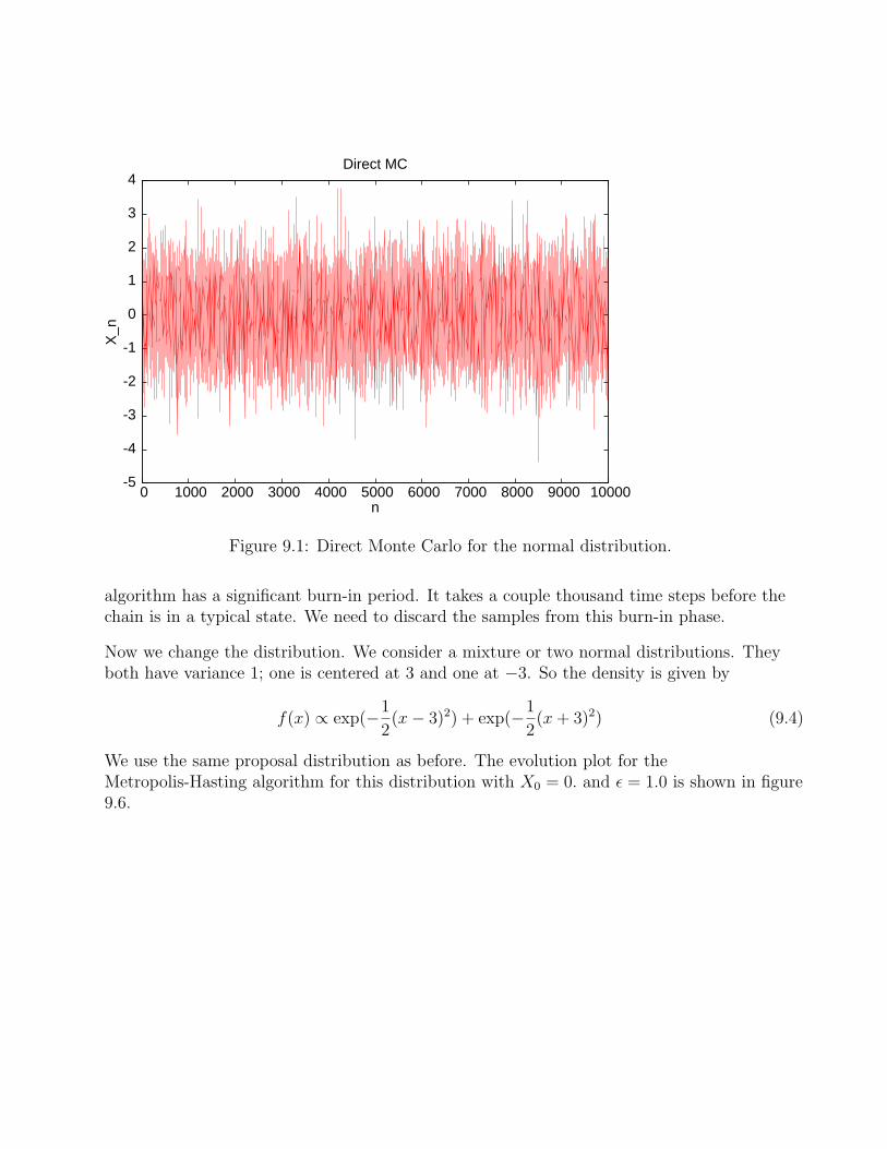
First consider what the evolution plot for direct MC would look like. So we just generatesample of Xn from the normal distribution. The evolution plot is shown in figure 9.1. Notethat there is not really any evolution here. Xn+1 has nothing to do with Xn.

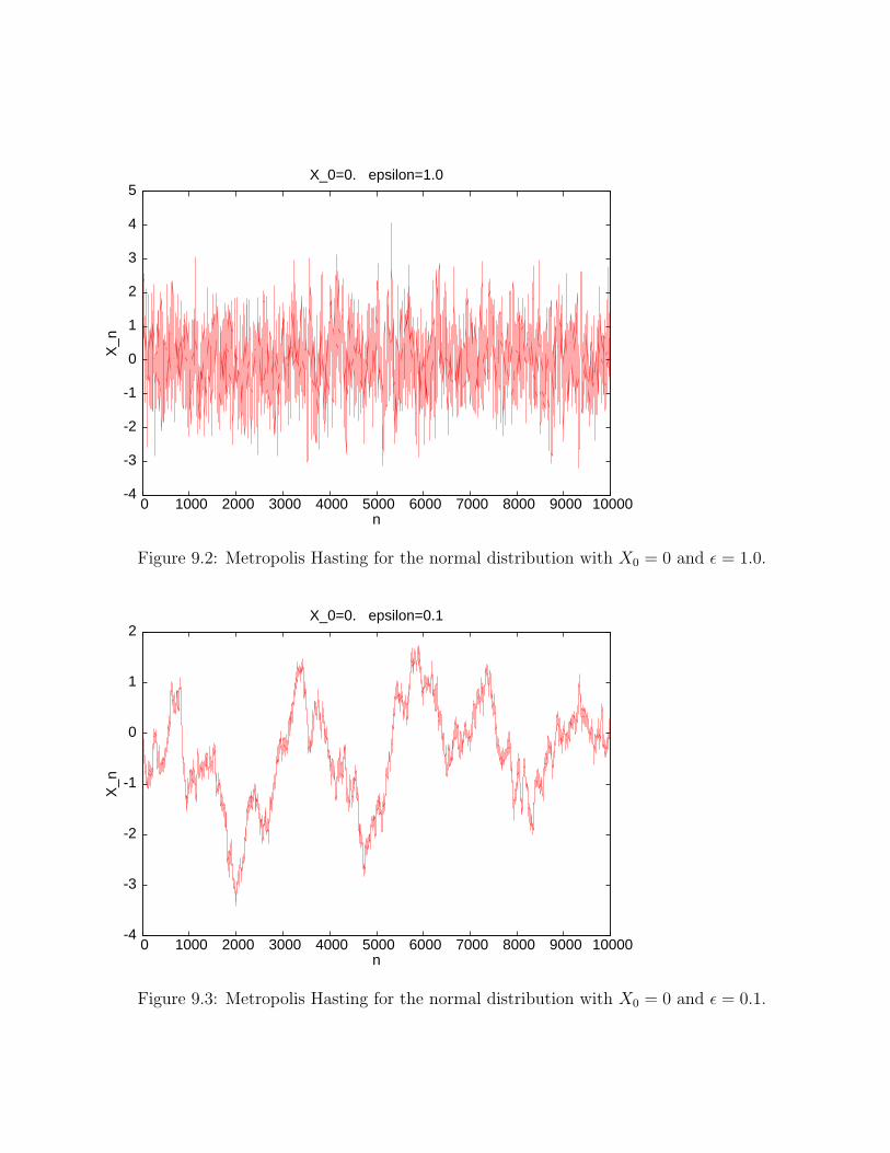
The next evolution plot (figure 9.2) is for the Metropolis-Hasting algorithm with X0 = 0. andǫ = 1.0. The algorithm works well with this initial condition and proposal distribution. Thesamples are correlated, but the Markov chain mixes well.

The next evolution plot (figure 9.3) is for the Metropolis-Hasting algorithm with X0 = 0. andǫ = 0.1. The algorithm does not mix as well with this proposal distribution. The state movesrather slowly through the state space and there is very strong correlation between the samplesover long times.

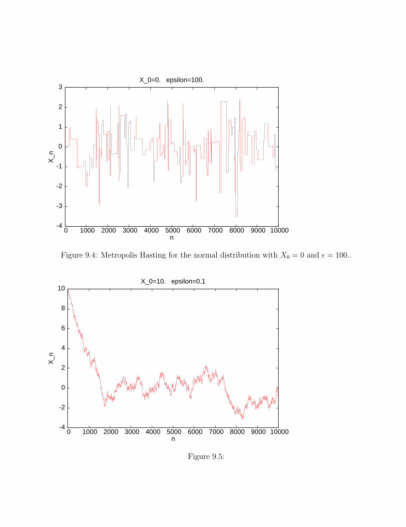
The next evolution plot (figure 9.4) is for the Metropolis-Hasting algorithm with X0 = 0. andǫ = 100.. This algorithm does very poorly. Almost all of the proposed jumps take the chain toa state with very low probability and so are rejected. So the chain stays stuck in the state itis in for many time steps. This is seen in the flat regions in the plot.

The next evolution plot (figure 9.5) is for the Metropolis-Hasting algorithm with X0 = 10.and ǫ = 0.1. Note that this initial value is far outside the range of typical values of X. This

-5

-4

-3

-2

-1

0

1

2

3

4

0 1000 2000 3000 4000 5000 6000 7000 8000 9000 10000

X_n

n

Direct MC

Figure 9.1: Direct Monte Carlo for the normal distribution.

algorithm has a significant burn-in period. It takes a couple thousand time steps before thechain is in a typical state. We need to discard the samples from this burn-in phase.

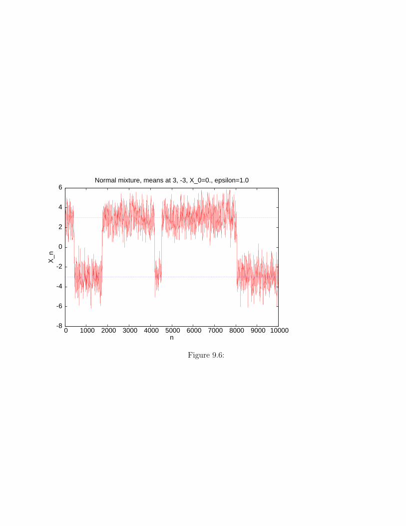
Now we change the distribution. We consider a mixture or two normal distributions. Theyboth have variance 1; one is centered at 3 and one at −3. So the density is given by

f(x) ∝ exp(−1

2(x− 3)2) + exp(−1

2(x+ 3)2) (9.4)

We use the same proposal distribution as before. The evolution plot for theMetropolis-Hasting algorithm for this distribution with X0 = 0. and ǫ = 1.0 is shown in figure9.6.

-4

-3

-2

-1

0

1

2

3

4

5

0 1000 2000 3000 4000 5000 6000 7000 8000 9000 10000

X_n

n

X_0=0. epsilon=1.0

Figure 9.2: Metropolis Hasting for the normal distribution with X0 = 0 and ǫ = 1.0.

-4

-3

-2

-1

0

1

2

0 1000 2000 3000 4000 5000 6000 7000 8000 9000 10000

X_n

n

X_0=0. epsilon=0.1

Figure 9.3: Metropolis Hasting for the normal distribution with X0 = 0 and ǫ = 0.1.

-4

-3

-2

-1

0

1

2

3

0 1000 2000 3000 4000 5000 6000 7000 8000 9000 10000

X_n

n

X_0=0. epsilon=100.

Figure 9.4: Metropolis Hasting for the normal distribution with X0 = 0 and ǫ = 100..

-4

-2

0

2

4

6

8

10

0 1000 2000 3000 4000 5000 6000 7000 8000 9000 10000

X_n

n

X_0=10. epsilon=0.1

Figure 9.5:

-8

-6

-4

-2

0

2

4

6

0 1000 2000 3000 4000 5000 6000 7000 8000 9000 10000

X_n

n

Normal mixture, means at 3, -3, X_0=0., epsilon=1.0

Figure 9.6:

9.2 The variance for correlated samples

We recall a few probability facts. The covarance of random variable X and Y is

cov(X, Y ) = E[XY ]− E[X]E[Y ] = E[(X − µX)(Y − µY )] (9.5)

This is a bi-linear form. Also note that cov(X,X) = var(X). Thus for any random variablesY1, · · · , YN ,

var(N∑

i=1

Yi) =1

N2

N∑

i,j=1

cov(Xi, Xj) (9.6)

A stochastic process Xn is said to be stationary if for all positive integers m and t, the jointdistribution of (X1+t, X2+t, · · · , Xm+t) is independent of t. In particular, cov(Xi, Xj) will onlydepends on |i− j|. It is not hard to show that if we start a Markov chain in the stationarydistribution, then we will get a stationary process. If the initial distribution is not thestationary distribution, then the chain will not be a stationary process. However, if the chainis irreducible, has a stationary distribution and is aperiodic, then the distribution of Xn willconverges to that of the stationary distribution. So if we only look at the chain at long timesit will be approximately a stationary process.

As before let

µ =1

N

N∑

n=1

f(Xn) (9.7)

be our estimator for the mean of f(X). Its variance is

V ar(µ) =1

N2

N∑

k,n=1

cov(f(Xk), f(Xn)) (9.8)

In the following we do a bit of hand-waving and make some unjustifiable assumptions. If theinitial state X0 is chosen according to the stationary distribution (which is typically impossiblein practice) then these assumptions are justified. But there are certainly situations wherethey are not. Let σ2(f) be the variance of f(X) in the stationary distribution. If N is large,then for most terms in the sum k and n are large. So the distribution of Xk and Xn should beclose to the stationary distribution. So the variance of f(Xk) should be close to σ(f)2. So

cov(f(Xk), f(Xn)) = [var(f(Xk))var(f(Xn))]1/2cor(f(Xk), f(Xn)) (9.9)

≈ σ2(f) cor(f(Xk), f(Xn)) (9.10)

where cor(Y, Z) is the correlation coefficient for Y and Z. Thus

V ar(µ) =σ(f)2

N2

N∑

k=1

N∑

n=1

cor(f(Xk), f(Xn)) (9.11)

Fix a k and think of cor(f(Xk), f(Xn)) as a function of n. This function will usually decay asn moves away from k. So for most values of k we can make the approximation

N∑

n=1

cor(f(Xk), f(Xn)) ≈∞∑

n=−∞

cor(f(Xk), f(Xk+n)) = 1 + 2∞∑

n=1

cor(f(Xk), f(Xk+n)) (9.12)

Finally we assume that this quantity is is essentially independent of k. This quantity is calledthe autocorrelation time of f(X). We denote it by τ(f). So

τ(f) = 1 + 2∞∑

n=1

cor(f(X0), f(Xn)) (9.13)

Explain why it is a “time” by looking at correlation that decays exponentially with a timescale. We now have

V ar(µ) ≈ σ(f)2

N2

N∑

k=1

τ(f) =σ(f)2τ(f)

N(9.14)

If the samples were independent the variance would be σ(f)2/N . So our result says that thisvariance for independent samples is increased by a factor of τ(f). Another way to interpretthis result is that the “effective” number of samples is N/τ(f).

To use this result we need to compute τ(f). We can use the simulation run to do this. Weapproximate the infinite sum in the expression for τ(f) by truncating it at M . So we need toestimate

1 + 2∞∑

n=1

cor(f(Xk), f(Xk+n)) (9.15)

ˆτ(f) = 1 + 21

N −M

N−M∑

k=1

M∑

n=1

cor(f(Xk), f(Xk+n)) (9.16)

Of course we do not typically have any a priori idea of how big M should be. So we need tofirst try to get an idea of how fast the correlation function decays.

MORE Help Help Help

Once we have an estimate for the variance of our estimator of E[f(X)], we can find aconfidence interval, i.e. error bars, in the usual way.

9.3 Variance via batched means

Esimating τ(f) can be tricky. In this section we give a quick and dirty method for puttingerror bars on our estimator that does not require computing the correlation time τ(f). Let N

be the number of MC time steps that we have run the simulation for. We pick an integer land put the samples in batches of length l. Let b = N/l. So b is the number of batches. Sothe first batch is X1, · · · , Xl, the second batch is Xl+1, · · · , X2l, and so on. If l is largecompared to the autocorrelation time of f(X), then if we pick Xi and Xj from two differentbatches then for most choices of i and j, f(Xi) and f(Xj) will be almost independent. So ifwe form estimators for the batches, j = 1, 2, · · · , b,

µj =1

l

b∑

i=1

f(X(j−1)l+i) (9.17)

then the µ1, · · · , µb will be almost independent. Note that

µ =1

b

b∑

i=1

µi (9.18)

So

var(µ) ≈ 1

b2

b∑

i=1

var(µi) (9.19)

The batches should have essentially the same distribution, so var(µi) should be essentiallyindependent of i. We estimate this common variance using the sample variance of µi,i = 1, 2, · · · , b. Denote it by s2l . Note that this batch variance depends very much on thechoice of l. Then our estimator for the variance of µ is

var(µ) ≈ s2lb

(9.20)

How do we choose the batch size? The number of batches b is N/l. We need b to be reasonablylarge (say 100, certainly at least 10) since we estimate the variance of the batches using asample of size b. So l should be at most 1/10 of N . We also need l to be large compared tothe autocorrelation time. If N is large enough, there will be a range of l where these twocriteria are both met. So for l in this range the estimates we get for the variance of µ will beessentially the same. So in practice we compute the above estimate of var(µ) for a range of land look for a range over which it is constant. If there is no such range, then we shouldn’t usebatched means. If this happens we should be suspicious of the MC simulation itself since thisindicates the number of MC time steps is not a large multiple of the autocorrelation time.

Stop - Wed, 4/6

We return to our hand-waving argument that the batch means should be almost independentif the batch size is large compared to the autocorrelation time and make this argument morequantitative.

The variance of µ is given exactly by

var(µ) =1

N2

N∑

i,j=1

cov(f(Xi), f(Xj)) (9.21)

Using batched means we approximate this by

1

b2

b∑

i=1

var(µi) (9.22)

This is equal to

1

N2

∑

(i,j)∈S

cov(f(Xi), f(Xj)) (9.23)

where S is the set of pairs (i, j) such that i and j are in the same batch. So the differencebetween the true variance of µ and what we get using batched means is

1

N2

∑

(i,j)/∈S

cov(f(Xi), f(Xj)) (9.24)

Keep in mind that the variance of µ is of order 1/N . So showing this error is small meansshowing it is small compared to 1/N . We fix the number b of batches, let N = bl and letl → ∞. We will show that in this limit the error times N goes to zero. So we consider

1

N

∑

(i,j)/∈S

cov(f(Xi), f(Xj)) (9.25)

Define C() by C(|i− j|) = cov(f(Xi), f(Xj)). Then the above can be bounded by

2b

N

l∑

k=1

∞∑

i=1

|C(i+ k)| (9.26)

Let

T (k) =∞∑

i=1

|C(i+ k)| =∞∑

i=k+1

|C(i)| (9.27)

We assume that C(i) is absolutely summable. So T (k) goes to zero as k → ∞. Using the factthat l = N/b, we have that the above equals

2

l

l∑

k=1

T (k) (9.28)

which goes to zero by the analysis fact that if limk→∞ ak = 0 then limn→∞1n

∑nk=1 ak = 0.

9.4 Subsampling

Until now we have always estimated the mean of f(X) with the estimator

µ =1

N

N∑

i=1

f(Xi) (9.29)

Subsampling (sometimes called lagging) means that we estimate the mean with

µsub =1

N/l

N/l∑

i=1

f(Xil) (9.30)

where l is the subsampling time. In other words we only evaluate f every l time steps.

One reason to do this is that if l is relatively large compared to the autocorrelation time, thenthe Xil will be essentially independent and we can estimate the variance of our estimator justas we did for direct Monte Carlo where the samples where independent. So the variance ofthe subsampling estimator will be approximately σ2/(N/l), where σ2 is the variance of f(X).

Intuitively one might expect if we compare two estimators, one with subsampling and onewithout, for the same number of MC steps, then the estimator without subsampling will dobetter. More precisely, we expect the variance of µ to be smaller than the variance of µsub ifwe use the same N in both. The following proposition makes this rigorous.

Proposition 1 Define µ as above and define

µj =1

N/l

N/l−1∑

i=0

f(Xil+j) (9.31)

Letting σ(?) denote the standard deviation of ?, we have

σ(µ) ≤ 1

l

l∑

j=1

σ(µj) (9.32)

Typically the variances of the µj will be essentially the same and so morally the propositionsays that the variance of µ is no larger than the variance of µsub.

Proof: The crucial fact used in the proof is that for any RV’s X, Y ,

|cov(X, Y )| ≤ [var(X) var(Y )]1/2 (9.33)

which follows from the Cauchy Schwarz inequality. Note that

µ =1

l

l∑

j=1

µj (9.34)

So

var(µ) =1

l2

l∑

i=1

l∑

j=1

cov(µi, µj) (9.35)

≤ 1

l2

l∑

i=1

l∑

j=1

[var(µi)var(µj)]1/2 (9.36)

=1

l2

l∑

i=1

l∑

j=1

σ(µi)σ(µj) (9.37)

=

[

1

l

l∑

i=1

σ(µi)

]2

(9.38)

Taking square roots the result follows. QED.

The proposition does not imply that it is never beneficial to subsample. Computing f forevery time step in the Markov chain takes more CPU time than subsampling with the samenumber of time steps. So there is a subtle trade-off between the increase in speed as wesubsample less frequently and the increase in the variance. Choosing l so large that it is muchlarger than the autocorrelation time is not necessarily the optimal thing to do. Ideally wewould like to choose l to minimize the error we get with a fixed amount of CPU time. Findingthis optimal choice of l is not trivial.

Factor of two hueristic: Actually finding the optimal amount choice of l is non-trivial. Wegive a crude method that at worst will require twice as much CPU time as the optimal choiceof l will. Let τf be time to compute f(Xi) and let τX be the time to perform one time step,i.e., compute Xi+1 given Xi. We take l to be τf/τX (rounded to an integer). Note that thiswill make the time spent on computing the Xi equal to the time spent evaluating f on the Xi.Now we argue that this is worse than by the optimal choice by at most a factor of two in CPUtime.

Let lopt be the optimal choice of l. First consider the case that l < lopt, i.e., we are evaluatingf more often than in the optimal case. Now compare a simulation with N time steps with ourcrude choice of l with a simulation with N time steps with the optimal choice lopt. They havethe same number of MC steps, but the simulation using l is sampled more often and so is atleast as accurate as the simulation using lopt. The simulation using l takes more CPU time,but at most the extra time is the time spent evaluating f and this is half of the total CPUtime. So the simulation using l takes at most twice as long as the one using lopt.

Now consider the case that l > lopt. Now we compare two simulations that each evaluate f atotal of M times. Since the evaluations using l are more widely spaced in time, they will beless correlated than those for the simulation using lopt. So the simulation using l will be atleast as accurate as the simulation using lopt. The two simulations evaluate f the samenumber of times. The simulation using l requires more MC steps. But the total time itspends computing the Xi is equal to the total time it spends evaluating f . So the total CPUis twice the time spent evaluating f . But the time spent evaluating f is the same for the twosimulations, and so is less that the total time the simulation using l uses.

9.5 Burn-in or initialization

In this section we consider the error resulting from the fact that we start the chain in anarbitrary state X0 which may be atypical is some sense. We need to run the chain for somenumber T of time steps and discard those times steps, i.e., we estimate the mean using

1

N − T

N∑

i=T+1

f(Xi) (9.39)

This goes under a variety of names: initilization, burn-in, convergence to stationarity,stationarization, thermalization.

We start with a trivial, but sometimes very relevant comment. Suppose we have a direct MCalgorithm that can generate a sample from the distribution we are trying to simulate, but it isreally slow. As long as it is possible to generate one sample in a not unreasonable amount oftime, we can use this algorithm to generate the inital state X0. Even if the algorithm thatdirectly samples from π takes a thousand times as much time as one step for the MCMCalgorithm, it may still be useful as a way to initialize the MCMC algorithm. When we can dothis we eliminate the burn-in or initialization issue altogether.

In the example of burn-in at the start of this chapter, f(X) was just X. When we started thechain in X0 = 10, this can be thought of as starting the chain in a state where the value off(X) is atypical. However, we should emphasize that starting in a state with a typical valueof f(X) does not mean we will not need a burn-in period. There can be atypical X for whichf(X) is typical as the following example shows.

Example: We want to simulate a nearest neighbor, symmetric random walk in onedimension with n steps. This is easily done by direct Monte Carlo. Instead we consider thefollowing MCMC. This is a 1d version of the pivot algorithm. This 1d RW can be thought ofas a sequence of n steps which we will denote by +1 and −1. So a state (s1, s2, · · · , sn) is astring of n +1’s and −1’s. Let f(s1, · · · , sn) =

∑ni=1 si, i.e., the terminal point of the random

walk. The probability measure we want is the uniform measure - each state has probability1/2n. The pivot algorithmn is as follows. Pick an integer j from 0, 1, 2, · · · , n− 1 with theuniform distribution. Leave si unchanged for i ≤ j and replace si by −si for i > j. Show thisstatisfies detailed balance.

In the following plots the number of steps in the walk is always L = 1, 000, 000. Allsimulations are run for 10,000 time steps. The initial state and the RV we look at varies.Note that all state have probability 2−n, so no state is atypical in the sense of havingunusually small probability.

In the first plot, figure 9.7, we start with the state that is n/2 +’s, followed by n/2 −’s. TheRV plotted is the distance of the endpoint to the origin. The signed distance to the endpointis approximately normal with mean zero and variance L. So the range of this RV is roughly[0, 2

√L]. In the initial state the RV is 0. This is a typical value for this RV. There is a

significant burn-in period.

0

50000

100000

150000

200000

250000

300000

0 1000 2000 3000 4000 5000 6000 7000 8000 9000 10000

X_n

n

RW distance to 0, L=1,000,000, atypical initial state

"rw_pivot1.plt"

Figure 9.7: MCMC simulation of random walk with L = 1, 000, 000 steps. Randomvariable plotted is distance from endpoint of walk to 0. Initial state is a walk thatgoes right for 500, 000 steps, then left for 500, 000 steps. MC is run for 10,000 timesteps. There is a significant burn-in period.

In the second plot, figure 9.8, the initial state is a random walk generated by just running adirect MC. The RV is still the distance from the endpoint to the origin. Note the difference invertical scale between this figure and the preceding figure. This MCMC seems to be working

well.

0

500

1000

1500

2000

2500

3000

3500

4000

4500

0 1000 2000 3000 4000 5000 6000 7000 8000 9000 10000

X_n

n

RW distance to 0, L=1,000,000, random initial state

Figure 9.8: MCMC simulation of random walk with L = 1, 000, 000 steps. Randomvariable plotted is distance from endpoint of walk to 0. Initial state is a random walkgenerated by direct sampling. MC is run for 10,000 time steps.

In the third plot, figure 9.9, the random variable is the distance the walk travels over the timeinterval [L/2, L/2 + 10, 000]. The initial state is again a random walk generated by justrunning a direct MC. For this RV the autocorrelation time is large.

There are two lessons to be learned from this example. One is the subtlety of initilization.The other is that there can be very different time scales in our MCMC. The autocorrelationtime of the RV that is the distance to the origin of the endpoint appears to be not very large.By contrast, the autocorrelation time for the other RV is rather large. We might expect thatthe exponential decay time for cov(f(Xi), f(Xj)) for the first RV will be not too large whilethis time for the second RV will be large. However, it is quitely like that for the first RV thereis some small coupling to this “slow mode.” So even for the first RV the true exponentialdecay time for the covariance may actually be quite large. Note that there are even slowermodes in this system. For example, consider the RV that is just the distance travelled overthe time interal [L/2, L/2 + 2].

A lot of theoretical discussions of burn-in go as follows. Suppose we start the chain in some

0

50

100

150

200

250

0 1000 2000 3000 4000 5000 6000 7000 8000 9000 10000

X_n

n

RW distance over [L/2,L/2+10,000], L=1,000,000, random initial state

Figure 9.9: MCMC simulation of random walk with L = 1, 000, 000 steps. Randomvariable plotted is distance walk travels over the time interval [L/2, L/2 + 10, 000].Initial state is a random walk generated by direct sampling.

distribution π0 and let πn be the distribution of Xn. Suppose we have a bound of the form

||πn − π||TV ≤ C exp(−n/τ) (9.40)

Then we can choose the number of samples T to discard by solving for T in C exp(−T/τ) ≤ ǫwhere ǫ is some small number. The problem is than we rarely have a bound of the aboveform, and in the rare cases when we do, the τ may be far from optimal. So we need apractical test for convergence to stationarity.

Stop - Wed, 4/6

If the distribution of the initial state X0 is the stationary (so the chain is stationary), thenthe two samples

f(X1), f(X2), · · · , f(XN), and f(XN+1), f(XN+2), · · · , f(X2N ) (9.41)

have the same distribution.

To use this observation to test for converges to stationarity, we let T be the number ofsamples we will discard for burn-in purposes and compare the two samples

f(XT+1), f(XT+2), · · · , f(XT+N), and f(XT+N+1), f(XT+N+2), · · · , f(XT+2N) (9.42)

A crude graphical test is just to plot histograms of these two samples and see if they areobviously different.

For a quantitative test we can use the Kolmogorov-Smirnov statistic. This is a slightlydifferent version of KS from the one we saw before when we tested if a sample came from aspecific distribution with a given CDF F . We first forget about the Markov chain andconsider a simpler situation. Let X1, X2, · · ·X2N be i.i.d. We think of this as two samples:X1, X2, · · ·XN and XN+1, XN+2, · · ·X2N . We form their empirical CDF’s:

F1(x) =1

N

N∑

i=1

1Xi≤x, (9.43)

F2(x) =1

N

2N∑

i=N+1

1Xi≤x (9.44)

Then we let

K = supx

|F1(x)− F2(x)| (9.45)

Note that K is a random variable (a statistic). As N → ∞, the distribution of√NK

converges. The limiting distribution has CDF

R(x) = 1−∞∑

k=1

(−1)k−1 exp(−2k2x2) (9.46)

This sum converges quickly and so R(x) is easily computed numerically. It is useful to knowthe 95% cutoff. We have R(1.36) = 0.95. So for large N , P (

√NK ≤ 1.36) ≈ 0.95.

Now return to MCMC. We cannot directly use the above since the samples of our Markovchain are correlated. So we must subsample. Let l be large compared to the autocorrelationtime for f , i.e., τ(f). Then we compare the two samples

f(XT+l), f(XT+2l), · · · , f(XT+Nl), and f(XT+Nl+l), f(XT+Nl+2l, · · · , f(XT+2Nl) (9.47)

Finally, we end this section by noting that it never hurts (much) to throw away the first 10%of your simulation run.

9.6 Autocorrelation times and related times

This section is based in large part on the article “The Pivot Algorithm: A Highly EfficientMonte Carlo Method for the Self-Avoiding Walk” by Madras and Sokal, Journal of StatisticalPhysics, 50, 109-186 (1988), sections 2.2.

We assume the Markov chain is discrete with a finite state space. Not all of the followingstatement extend to the case of continuous state space or infinite discrete state space. We alsoassume our chain is irrecducible and aperiodic.

In this section we study three different times that can be defined for an MCMC and how theyare related. We have already seen one autocorrelation time defined by (9.13). In this sectionwe will refer to this as an “integrated autocorrelation time” and write it as τint,f . We recallthe formula for it:

τint,f = 1 + 2∞∑

n=1

cor(f(X0), f(Xn)) (9.48)

This time is important since it enters our formula for the variance of our estimator µ. Thatvariance is given approximatly by σ(f)2τint,f/N . Since the variance for direct Monte Carlo isσ(f)2/N , we can interpret this formula as saying that in an MCMC the number of effectivelyindependent samples is N/τ(f). (The definition of τint,f in Madras and Sokal differs by afactor of 2.) In the definition of τint,f we assume that X0 is distributed according to thestationary distribution. So the Markov chain is stationary. (We can imagine that we have runthe chain for a sufficiently long burn-in period to achieve this. In that case X0 is the stateafter the burn-in period.)

The second time we will consider is closely related. We follow the terminology of Madras andSokal. For a function f on the state space we define the unnormalized autocorrelationfunction of f to be

Cf (t) = E[f(Xs)f(Xs+t)]− µ2f , where (9.49)

µf = E[f(Xs)] (9.50)

Note that Cf (0) is the variance of f(Xt). We define the normalized autocorrelation functionto be

ρf (t) =Cf (t)

Cf (0)(9.51)

With our assumptions on the Markov chain ρf (t) will decay exponentially with t. We definethe exponential autocorrelation time for f by

τexp,f = lim supt→∞

t

−log|ρf (t)|(9.52)

We define an exponential autocorrelation time for the entire chain by

τexp = supf

τexp,f (9.53)

With our assumptions on the Markov chain, τf will be finite, but it can be infinite when thestate space is finite.

The two times we have considered so far are properties of the stationary Markov chain. Thethird time characterizes how long it takes the Markov chain to converge to the stationarydistribution starting from an arbitrary initial condition. With our assumptions on the chainthis convergence will be exponentially fast. We define τconv to be the slowest convergence ratewe see when we consider all initial distributions. More precisely we define

τconv = supπ0

lim supt→∞

t

− log(||πt − π||TV )(9.54)

Here π0 is the distribution of X0, πt is the distribution of Xt and π is the stationarydistribution.

The following two propositions almost say that τexp = τconv.

Proposition 2 Suppose there are constants c and τ such that for all initial π0,

||πt − π||TV ≤ ce−t/τ (9.55)

Then τexp ≤ τ .

Remark: This almost says τexp ≤ τconv. It does not exactly say this since our definition ofτconv does not quite imply the bound (9.55) holds with τ = τconv.

Proof: If we apply the hypothesis to the initial condition where π0 is concentrated on thesingle state x, we see that

||pt(x, ·)− π(·)||1 ≤ ce−t/τ (9.56)

Now let f be a function on the state space with zero mean in the stationary distribution.Then using

∑

y f(y)π(y) = 0, we have

|E[f(X0)f(Xt)]| = |∑

x,y

f(x)π(x)pt(x, y)f(y)| (9.57)

= |∑

x,y

f(x)π(x)f(y)[pt(x, y)− π(y)]| (9.58)

≤∑

x

|f(x)|π(x)||f ||∞||pt(x, ·)− π(·)||1 (9.59)

≤∑

x

|f(x)|π(x)||f ||∞ce−t/τ (9.60)

The propostion follows. QED.

Proposition 3 Suppose there are constants c and τ such that

Cov(g(X0), f(Xt)) ≤ ce−t/τ ||f ||∞||g||∞ (9.61)

for all functions f and g on the state space. Then τconv ≤ τ .

Remark: This almost says τconv ≤ τexp. It does not exactly say this since our definition ofτexp does not quite imply the bound (9.61) holds with τ = τexp.

Proof: The total variation norm can be computed by

||πt − π||TV supf :||f ||∞≤1

∑

x

f(x)[πt(x)− π(x)] (9.62)

Let g(x) = π0(x)/π(x). (Note that π(x) > 0 for all x.) The expected value of g is thestationary distribution is

Eg(Xt) =∑

x

g(x)π(x) =∑

x

π0(x) = 1 (9.63)

So

Cov(g(X0), f(Xt)) =∑

x,y

g(x)f(y)π(x)pt(x, y)− E[g(X0)]E[f(Xt)] (9.64)

=∑

x,y

π0(x)f(y)pt(x, y)− E[f(Xt)] (9.65)

=∑

y

πt(y)f(y)−∑

x

π(x)f(x) (9.66)

Since this is bounded by ce−t/τ ||f ||∞||g||∞ = ce−t/τ ||g||∞, the proposition follows. QED.

Recall that the stationary distribution is a left eigenvector of the transition matrix p(x, y),and the constant vector is a right eigenvector. (Both have eigenvalue 1.) In general p(x, y) isnot symmetric, so there need not be a complete set of left or right eigenvectors. However, ifthe chain satisfies detailed balance then there is, as we now show. We rewrite the detailedbalance condition as

π(x)1/2p(x, y)π(y)−1/2 = π(y)1/2p(x, y)π(y)−1/2 (9.67)

So if we define

p(x, y) = π(x)1/2p(x, y)π(y)−1/2 (9.68)

then p is symmetric. (p is self-adjoint on l2(π).) If we let S be the linear operator onfunctions on the state space that is just multiplication by π1/2, then

p = SpS−1 (9.69)

Let ek be a complete set of eigenvectors for it. So pek = λkek. Note that the ek areorthonormal.

Now let f(x) be a function on the state space. It suffices to consider functions which havezero mean in the stationary distribution. So the covariance is just E[f(X0)f(Xt)]. Tocompute this expected value we need the joint distribution of X0, Xt. It is π(x0)p

t(x0, xt). So

E[f(X0)f(Xt)] =∑

x0,xt

π(x0)pt(x0, xt)f(x0)f(xt) =

∑

x0

f(x0)π(x0)∑

xt

pt(x0, xt)f(xt) (9.70)

We can write this as

(fπ, ptf) = (fπ, (S−1pS)tf) = (fπ, S−1ptSf) = (S−1πf, ptSf) = (fπ1/2, ptπ1/2f) (9.71)

Using the spectral decompostion of p this is∑

k

(fπ1/2, ek)λtk(ek, π

1/2f) =∑

k

c2kλtk (9.72)

with ck = (fπ1/2, ek).

The right eigenvector of p with eigenvalue 1 is just the constant vector. So π1/2 is theeigenvector of p with eigenvalue 1. So

c1 =∑

x

π(x)1/2π(x)1/2f(x) = 0 (9.73)

since the mean of f in the stationary distribution is zero. Let λ be the maximum of theabsolute values of the eigenvalues not equal to 1. So for k ≥ 2, |λt

k| ≤ λ. So

E[f(X0)f(Xt)] ≤ λt∑

k≥2

c2k (9.74)

Note that var(f(X0)) =∑

k c2k. So

τint,f = 1 + 2∞∑

t=1

cor(f(X0), f(Xt)) ≤ 1 + 2∞∑

t=1

λt = 1 + 2λ

1− λ=

1 + λ

1− λ≤=

2

1− λ(9.75)

Stop - Mon, 4/11

Proposition 4 Assume that p is diagonalizable. Let λ be the maximum of the absolute values

of the eigenvalues not equal to 1. Then τconv is given by λ = exp(−1/τconv).

Proof: Let S be an invertible matrix that diagonalizes p. So p = SDS−1 where D is diagonalwith entries λk. We order things so that the first eigenvalue is 1. We have πp = π. SoπSD = πS. So πS is an eigenvector of D with eigenvalue 1. So it must be (1, 0, · · · , 0). Soπ = (1, 0, · · · , 0)S−1. This says that the first row of S−1 is π. If we let ~1 be the column vector(1, 1, · · ·)T , then we know p~1 = ~1. So DS−1~1 = S−1~1. This says S−1~1 is the eigenvector of Dwith eigenvalue 1, so it is (1, 0, · · · , 0)T . So ~1 = S(1, 0, · · · , 0)T . We now have

πt = π0pt = π0(SDS−1)t = π0SD

tS−1 = π0Sdiag(λt1, · · · , λt)S−1 (9.76)

= π0Sdiag(1, 0, 0 · · · , 0)S−1 + π0Sdiag(0, λt2, · · · , λt)S−1 (9.77)

Since ~1 = S(1, 0, · · · , 0)T , Sdiag(1, 0, · · ·) is the matrix with 1’s in the first column and 0’selsewhere. So π0Sdiag(1, 0, 0 · · · , 0) is just (1, 0, · · · , 0)T Thus π0Sdiag(1, 0, 0 · · · , 0)S−1 = π.The second term in the above goes to zero like λt. QED

Now consider the bound τint,f ≤ 21−λ

which we derived when the chain satistifed detailedbalance. Using the previous proposition, this becomes

τint,f ≤ 2

1− exp(−1/τconv)(9.78)

If τconv is large, then the right side is approximately 2τconv.

Madras and Sokal carry out a detailed analysis for the pivot algorithm for a random walk intwo dimensions. Then show that τexp is O(N). For “global” random variables such as thedistance from the origin to the end of the walk, τf,int is O(log(N)). But for very localobservables, such as the angle between adjacent steps on the walk, τf,int is O(N).

9.7 Missing mass or bottlenecks

The problem we briefly consider in this section is an MCMC in which the state space can bepartitioned into two (or more) subsets S = S1 ∪ S2 such that although the probabilities ofgetting from S1 to S2 and from S2 to S1 are not zero, they are very small.

The worst scenario is that we start the chain in a state in one of the subsets, say S1, and itnever leaves that subset. Then our long time sample only samples S1. Without any aprioriknowledge of the distribution we want to simulate, there is really no way to know if we are

failing to sample a representative portion of the distribution. “You only know what you haveseen.”

The slightly less worse scenario is that the chain does occasionally make transitions betweenS1 and S2. In this case there is no missing mass, but the autocorrelation time will be huge. Inparticular it will be impossible to accurately estimate the probabilities of S1 and S2.

It is worth looking carefully at the argument that your MCMC is irreducible to see if you cansee some possible “bottlenecks”.

If a direct MC is possible, although slow, we can do a preliminary direct MC simulation to geta rough idea of where the mass is.

Missing mass is not just the problem that you fail completely to visit parts of the state space,there is also the problem that you do eventually visit all of the state space, but it takes a longtime to get from some modes to other modes. One way to test for this is to run multipleMCMC simulations with different initial conditions.

In the worst scenario when the chain is stuck in one of the two subsets, it may appear thatthere is a relatively short autocorrelation time and the burn-in time is reasonable. So ourestimate of the autocorrelation time or the burn-in time will not indicate any problem.However, when the chain does occassionally make transitions between modes, we will see avery long autocorrelation time and a very slow convergence to stationary. So our tests forthese sources of errors will hopefully alert us to the bottleneck.