chapter 8 – comparing congestion control regimes in a
TRANSCRIPT
Chapter 8 – Comparing Congestion Control Regimes in a Heterogeneous Network

Study of Proposed Internet Congestion Control Mechanisms NIST
Mills, et al. Special Publication 500-282 316
8 Comparing Congestion Control Regimes in a Heterogeneous Network In this chapter, we investigate effects on macroscopic behavior and user experience when deploying various congestion control algorithms in a simulated, heterogeneous network, i.e., a network that includes flows operating under normal TCP congestion control procedures together with flows operating under one of seven proposed alternate congestion control algorithms, as identified in Table 8-1. Mixing alternate congestion control regimes together with standard TCP will enable us to investigate the influence of alternate congestion avoidance algorithms on the performance of TCP flows. We also introduce additional flow sizes to represent downloading movies and software updates (e.g., service packs). These file sizes augment the Web objects and document downloads used in previous experiments (Chapters 6 and 7). Here, we adopt a small-scale network, similar to that used in Chapter 7, because earlier experiments suggested that a small-scale network yields significant information while requiring fewer resources. Reducing computational cost allows us to repeat our experiments first with a large initial slow-start threshold and then with a small initial slow-start threshold. We take this step in light of the apparent significance of the initial slow-start threshold, as uncovered in earlier experiments.
Table 8-1. Alternate Congestion Control Regimes Compared
Identifier Label Name of Congestion Avoidance Algorithm1 BIC Binary Increase Congestion Control2 CTCP Compound Transmission Control Protocol
3 FAST Fast Active-Queue Management Scalable Transmission Control Protocol
4 FAST-AT FAST with -tuning Enabled
5 HSTCP High-Speed Transmission Control Protocol6 HTCP Hamilton Transmission Control Protocol7 Scalable Scalable Transmission Control Protocol
We exposed our simulated network to a range of congestion conditions, but we
reduced overall congestion by an order of magnitude from previous experiments. We made this reduction in order to investigate behavior of the alternate congestion control algorithms under little to modest congestion, which should reveal any differences in user experience when large files are sent over fast paths between sources and receivers with high-speed network interfaces. In fact, we classified flows into groups based on four dimensions: (1) congestion control algorithm used; (2) characteristics of the network path transited; (3) minimum interface speed of the source and receiver pair; and (4) size of the transferred file. Such classification enabled us to compare relative performance among congestion control algorithms for specific flow groups. We collected and compared data representing the distribution of goodput for users of flows in each flow group.
Study of Proposed Internet Congestion Control Mechanisms NIST
Mills, et al. Special Publication 500-282 317
We organize what follows into six sections. Sec. 8.1 describes the experiment design, including robustness factors, fixed factors, conditions simulated and responses measured. In describing the design, we explain how we controlled the generation of flows in each group. Sec. 8.1 also gives the domain view of the simulated conditions. Sec. 8.2 details resource requirements for simulating the experiments and outlines how we collected and summarized experiment data. Sec. 8.3 explains the data analysis approach we used to investigate experiment responses. Sec. 8.4 presents the results from both sets of experiments, that is, with a large and a small initial slow-start threshold. Sec. 8.5 discusses key findings from the results. We conclude in Sec. 8.6.
8.1 Experiment Design We conducted these experiments within the same fixed, heterogeneous topology (see Fig. 6-1) used in previous experiments. As discussed below, we employed nine robustness factors, which define the range over which our findings apply. We fixed the remaining model parameters and then created a design template to simulate 32 conditions. We repeated the 32 simulated conditions a second time after lowering the initial slow-start threshold, so the simulations yielded two sets of results. By mixing flows using alternate congestion control algorithms together with flows using standard TCP, we can examine the relative influence of the various alternate algorithms on normal TCP flows. Such information could be useful because the Internet is unlikely to cutover all at once to an alternate congestion control algorithm, but rather will experience a transition period during which TCP flows will coexist with flows using alternate algorithms.
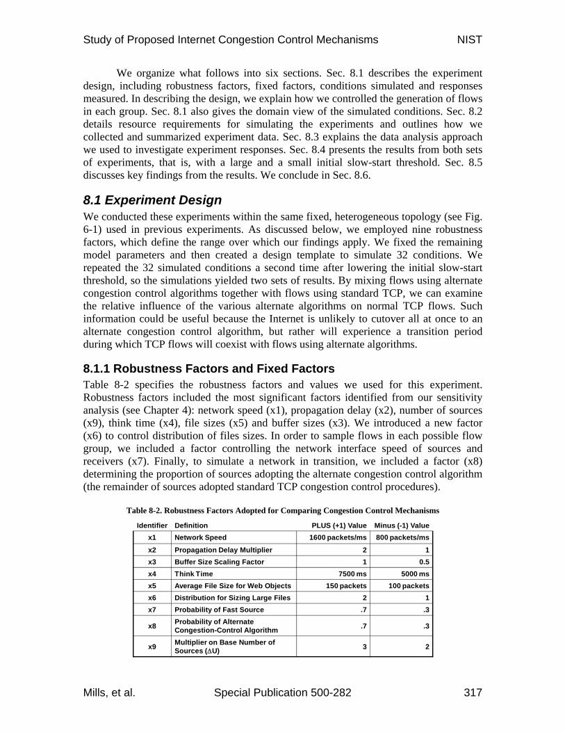
8.1.1 Robustness Factors and Fixed Factors Table 8-2 specifies the robustness factors and values we used for this experiment. Robustness factors included the most significant factors identified from our sensitivity analysis (see Chapter 4): network speed (x1), propagation delay (x2), number of sources (x9), think time (x4), file sizes (x5) and buffer sizes (x3). We introduced a new factor (x6) to control distribution of files sizes. In order to sample flows in each possible flow group, we included a factor controlling the network interface speed of sources and receivers (x7). Finally, to simulate a network in transition, we included a factor (x8) determining the proportion of sources adopting the alternate congestion control algorithm (the remainder of sources adopted standard TCP congestion control procedures).
Table 8-2. Robustness Factors Adopted for Comparing Congestion Control Mechanisms
Identifier Definition PLUS (+1) Value Minus (-1) Valuex1 Network Speed 1600 packets/ms 800 packets/ms
x2 Propagation Delay Multiplier 2 1x3 Buffer Size Scaling Factor 1 0.5x4 Think Time 7500 ms 5000 msx5 Average File Size for Web Objects 150 packets 100 packetsx6 Distribution for Sizing Large Files 2 1x7 Probability of Fast Source .7 .3
x8 Probability of Alternate Congestion-Control Algorithm .7 .3
x9 Multiplier on Base Number of Sources ( U) 3 2
Study of Proposed Internet Congestion Control Mechanisms NIST
Mills, et al. Special Publication 500-282 318
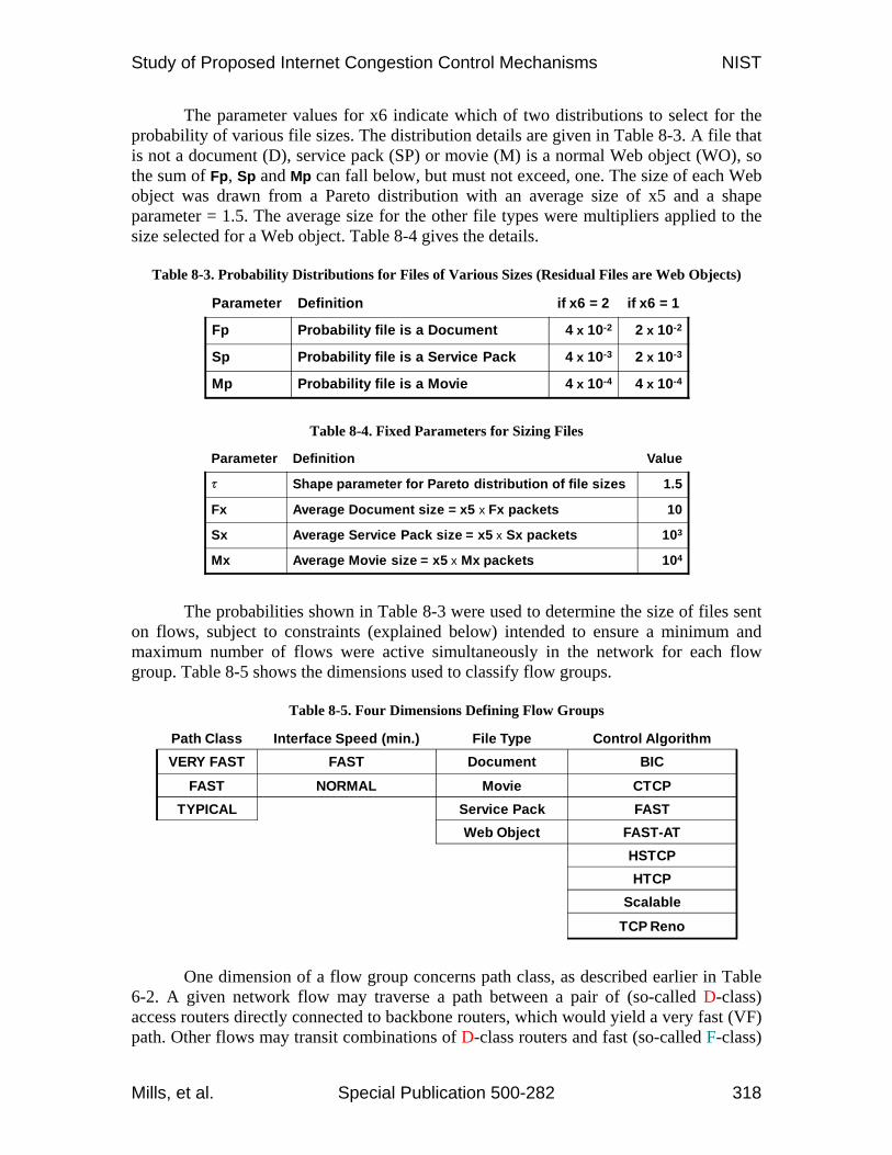
The parameter values for x6 indicate which of two distributions to select for the probability of various file sizes. The distribution details are given in Table 8-3. A file that is not a document (D), service pack (SP) or movie (M) is a normal Web object (WO), so the sum of Fp, Sp and Mp can fall below, but must not exceed, one. The size of each Web object was drawn from a Pareto distribution with an average size of x5 and a shape parameter = 1.5. The average size for the other file types were multipliers applied to the size selected for a Web object. Table 8-4 gives the details.
Table 8-3. Probability Distributions for Files of Various Sizes (Residual Files are Web Objects)
Parameter Definition if x6 = 2 if x6 = 1
Fp Probability file is a Document 4 x 10⁻² 2 x 10⁻²
Sp Probability file is a Service Pack 4 x 10⁻³ 2 x 10⁻³
Mp Probability file is a Movie 4 x 10⁻⁴ 4 x 10⁻⁴
Table 8-4. Fixed Parameters for Sizing Files
Parameter Definition Value
Shape parameter for Pareto distribution of file sizes 1.5
Fx Average Document size = x5 x Fx packets 10
Sx Average Service Pack size = x5 x Sx packets 103
Mx Average Movie size = x5 x Mx packets 104
The probabilities shown in Table 8-3 were used to determine the size of files sent
on flows, subject to constraints (explained below) intended to ensure a minimum and maximum number of flows were active simultaneously in the network for each flow group. Table 8-5 shows the dimensions used to classify flow groups.
Table 8-5. Four Dimensions Defining Flow Groups
Path Class Interface Speed (min.) File Type Control AlgorithmVERY FAST FAST Document BIC
FAST NORMAL Movie CTCPTYPICAL Service Pack FAST
Web Object FAST-ATHSTCPHTCP
Scalable
TCP Reno
One dimension of a flow group concerns path class, as described earlier in Table
6-2. A given network flow may traverse a path between a pair of (so-called D-class) access routers directly connected to backbone routers, which would yield a very fast (VF) path. Other flows may transit combinations of D-class routers and fast (so-called F-class)

Study of Proposed Internet Congestion Control Mechanisms NIST
Mills, et al. Special Publication 500-282 319
access routers, which yield fast (F) paths. Any flows traversing at least one normal (so-called N-class) access router would travel on a typical (T) path. A second dimension of a flow group considers the speed with which a source-receiver pair connects to the network. A flow can operate no faster than the minimum speed of the source and receiver, which may connect at a normal speed (e.g., 100 Mbps) or fast speed (e.g., 1 Gbps). If both source and receiver have fast network connections, then the interface speed is fast (F); otherwise, the interface speed is normal (N). A third dimension of a flow group is file type, which denotes file size. Flows with smaller files (e.g., Web objects) usually achieve lower goodputs because a larger portion of the flow lifetime is spent establishing the maximum transfer rate. In fact, sufficiently short files may end before a flow even reaches the maximum achievable transfer rate on a path. The fourth dimension of a flow group identifies the congestion control algorithm used by the source that originates the flow. Since each simulation had a mix of TCP sources and alternate sources, the fourth dimension in a given experiment execution took on two values: TCP Reno and one of the remaining congestion control algorithms. Flows, originated by TCP Reno sources and alternate sources, fell into one of 24 flow groups, depending on the values for the remaining three dimensions: path class, interface speed and file type. Table 8-6 identifies these 24 flow groups.
Table 8-6. Flow Group Identifiers Assigned Based on Three-Dimensional Classification
Web ObjectNORMALTYPICAL24
Web ObjectFASTTYPICAL23
Web ObjectNORMALFAST22
Web ObjectFASTFAST21
Web ObjectNORMALVERY FAST20
Web ObjectFASTVERY FAST19
DocumentNORMALTYPICAL18
DocumentFASTTYPICAL17
DocumentNORMALFAST16
DocumentFASTFAST15
DocumentNORMALVERY FAST14
DocumentFASTVERY FAST13
Service PackNORMALTYPICAL12
Service PackFASTTYPICAL11
Service PackNORMALFAST10
Service PackFASTFAST9
Service PackNORMALVERY FAST8
Service PackFASTVERY FAST7
MovieNORMALTYPICAL6
MovieFASTTYPICAL5
MovieNORMALFAST4
MovieFASTFAST3
MovieNORMALVERY FAST2
MovieFASTVERY FAST1
File TypeInterface SpeedPath ClassIdentifier

Study of Proposed Internet Congestion Control Mechanisms NIST
Mills, et al. Special Publication 500-282 320
8.1.1.1 Constraints on Flows of Large Size. Applying probabilities associated with factor x6 (distribution for sizing larger files) could lead to two undesirable consequences: too few samples on very fast paths and too many samples on typical paths. If the probabilities of very large files, e.g., movies and service packs, were sufficiently small, then a given experiment may generate few or no large files for some rarer combinations of flow traits, e.g., flows with fast interface speeds traveling over very fast paths. On the other hand, the probabilities of very large files may also cause a simulated network to be swamped with many large files that take much time to transfer on flows with normal interface speeds traversing typical paths. In such cases, large files flowing over slow paths can accumulate in the network because each of the file transfers takes a long time to complete and the more such flows in the network, the longer each takes to complete.1
The problem of too few samples might be addressed by simulating longer network evolution, but the processing cost for the additional simulated time could prove prohibitive. The problem of too many samples cannot be solved by simulating longer network evolution; in fact, simulating longer evolution would increase accumulation of large files being transferred on flows transiting slow paths. For these reasons, we decided to place constraints on the generation of file types with large sizes. The aim of these constraints was to ensure a sufficient number of flow samples in each flow group, while not overwhelming the network with flows that accumulate in any particular group.
In short, using factor x6 we computed a target maximum number of active flows for each file type, other than Web objects, i.e., for movies, service packs and documents. Based on relevant factors (x7 and x8) we also computed a target minimum number of active flows for each type. During simulation, each originating flow was assigned a preliminary file type of Web object. A file size was drawn from a Pareto distribution with a specified average (x5) and shape ( ). A check was then made to see if the minimum number of movies was active on flows with matching path class, interface speed and congestion control algorithm. If not, then the flow was assigned a file type of movie and the file size was increased by the appropriate multiplier taken from Table 8-4; otherwise, a similar check was made for service pack and then, if necessary, document. If the minimum number of flows was active in all three possible flow groups (designated by a specific path class, interface speed and congestion control algorithm in combination with one of the larger file types), then a file type was selected based on the specified probability distribution (x6). If the target maximum number of flows was already active for the selected file type, then the flow remained a Web object; otherwise, the flow size was increased by the appropriate multiplier.
Computing the target maximum number of active flows for specific file types is straightforward. For example, given the total number (s) of sources in a simulation we computed the target number of active document flows as follows.
(1)
1 In a real network the problem of too many large flows over specific paths could be ameliorated by users aborting flows observed to be running too slowly or taking too long. This would not be true for unattended flows, such as appear in typical peer-to-peer applications. The simulations used in these experiments include only unattended flows, so one cannot rely on users to abort slow flows. Note that MesoNet does include the possibility of user-attended flows in addition to unattended flows.
sDCMAX max ceil s Fp×( ) 1000,( )≡
Study of Proposed Internet Congestion Control Mechanisms NIST
Mills, et al. Special Publication 500-282 321
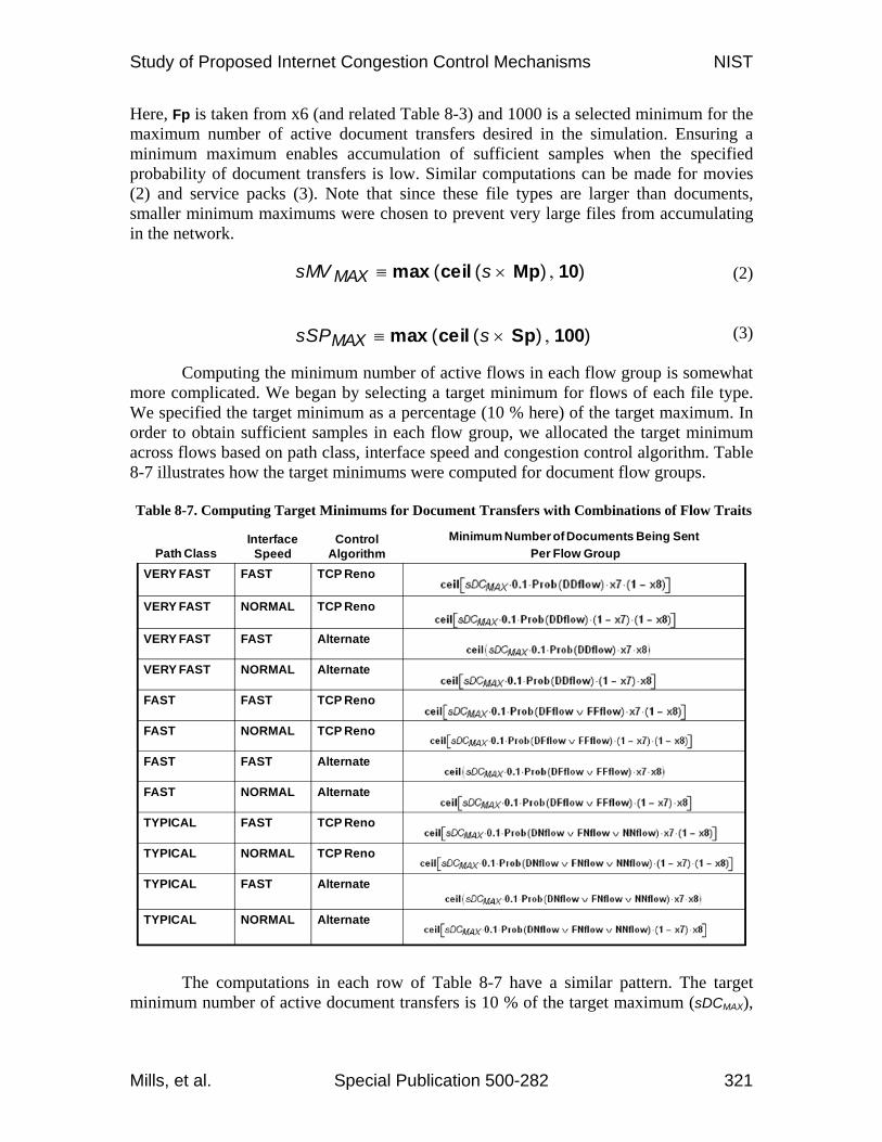
Here, Fp is taken from x6 (and related Table 8-3) and 1000 is a selected minimum for the maximum number of active document transfers desired in the simulation. Ensuring a minimum maximum enables accumulation of sufficient samples when the specified probability of document transfers is low. Similar computations can be made for movies (2) and service packs (3). Note that since these file types are larger than documents, smaller minimum maximums were chosen to prevent very large files from accumulating in the network.
(2)
(3)
Computing the minimum number of active flows in each flow group is somewhat more complicated. We began by selecting a target minimum for flows of each file type. We specified the target minimum as a percentage (10 % here) of the target maximum. In order to obtain sufficient samples in each flow group, we allocated the target minimum across flows based on path class, interface speed and congestion control algorithm. Table 8-7 illustrates how the target minimums were computed for document flow groups. Table 8-7. Computing Target Minimums for Document Transfers with Combinations of Flow Traits
Path ClassInterface
SpeedControl
AlgorithmMinimum Number of Documents Being Sent
Per Flow GroupVERY FAST FAST TCP Reno
VERY FAST NORMAL TCP Reno
VERY FAST FAST Alternate
VERY FAST NORMAL Alternate
FAST FAST TCP Reno
FAST NORMAL TCP Reno
FAST FAST Alternate
FAST NORMAL Alternate
TYPICAL FAST TCP Reno
TYPICAL NORMAL TCP Reno
TYPICAL FAST Alternate
TYPICAL NORMAL Alternate
The computations in each row of Table 8-7 have a similar pattern. The target minimum number of active document transfers is 10 % of the target maximum (sDCMAX),
sMV MAX max ceil s Mp×( ) 10,( )≡
sSPMAX max ceil s Sp×( ) 100,( )≡
Study of Proposed Internet Congestion Control Mechanisms NIST
Mills, et al. Special Publication 500-282 322
but multiplied by: (a) the probability that a flow transits a given path class2, e.g., Prob(DDflow), (b) the probability a flow connects with a particular interface speed (x7 or 1-x7) and (c) the probability a flow uses a specified congestion control algorithm (x8 or 1-x8). Similar computations can be made for movies and service packs.
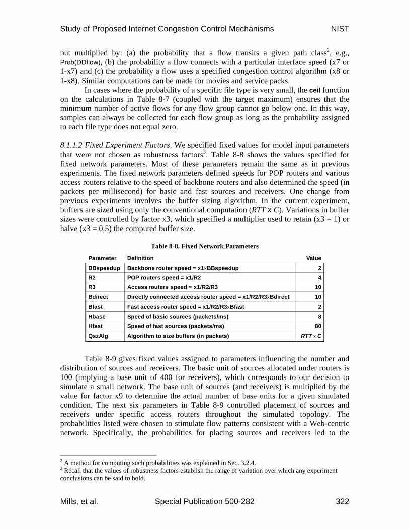
In cases where the probability of a specific file type is very small, the ceil function on the calculations in Table 8-7 (coupled with the target maximum) ensures that the minimum number of active flows for any flow group cannot go below one. In this way, samples can always be collected for each flow group as long as the probability assigned to each file type does not equal zero. 8.1.1.2 Fixed Experiment Factors. We specified fixed values for model input parameters that were not chosen as robustness factors3. Table 8-8 shows the values specified for fixed network parameters. Most of these parameters remain the same as in previous experiments. The fixed network parameters defined speeds for POP routers and various access routers relative to the speed of backbone routers and also determined the speed (in packets per millisecond) for basic and fast sources and receivers. One change from previous experiments involves the buffer sizing algorithm. In the current experiment, buffers are sized using only the conventional computation (RTT x C). Variations in buffer sizes were controlled by factor x3, which specified a multiplier used to retain (x3 = 1) or halve (x3 = 0.5) the computed buffer size.
Table 8-8. Fixed Network Parameters
Parameter Definition Value
BBspeedup Backbone router speed = x1xBBspeedup 2R2 POP routers speed = x1/R2 4R3 Access routers speed = x1/R2/R3 10Bdirect Directly connected access router speed = x1/R2/R3xBdirect 10Bfast Fast access router speed = x1/R2/R3xBfast 2
Hbase Speed of basic sources (packets/ms) 8Hfast Speed of fast sources (packets/ms) 80
QszAlg Algorithm to size buffers (in packets) RTT x C
Table 8-9 gives fixed values assigned to parameters influencing the number and
distribution of sources and receivers. The basic unit of sources allocated under routers is 100 (implying a base unit of 400 for receivers), which corresponds to our decision to simulate a small network. The base unit of sources (and receivers) is multiplied by the value for factor x9 to determine the actual number of base units for a given simulated condition. The next six parameters in Table 8-9 controlled placement of sources and receivers under specific access routers throughout the simulated topology. The probabilities listed were chosen to stimulate flow patterns consistent with a Web-centric network. Specifically, the probabilities for placing sources and receivers led to the
2 A method for computing such probabilities was explained in Sec. 3.2.4. 3 Recall that the values of robustness factors establish the range of variation over which any experiment conclusions can be said to hold.

Study of Proposed Internet Congestion Control Mechanisms NIST
Mills, et al. Special Publication 500-282 323
distribution4 shown in Table 8-10, where most sources were placed under fast access routers and a preponderance of receivers were placed under normal access routers. This led to a distribution of flows across flow classes with the approximate probabilities listed in Table 8-11. About 94 % of flows transited at least one N-class access router, with those flows partitioned as follows: 55 % transited FN paths, 32 % crossed NN paths and 7 % traversed DN paths.
Table 8-9. Fixed Source and Receiver Parameters Parameter Definition Value
Bsources Basic unit for sources per access router 100
P(Ns) Probability source under normal access router 0.1
P(Nsf) Probability source under fast access router 0.6
P(Nsd) Probability source under directly connected access router 0.3
P(Nr) Probability receiver under normal access router 0.6
P(Nrf) Probability receiver under fast access router 0.2
P(Nrd) Probability receiver under directly connected access router 0.2
sstINT Initial slow-start threshold (packets) 231/2 or 100
Table 8-10. Proportion of Sources and Receivers Placed under Specific Router Classes
Table 8-11. Approximate Probability of Flows Transiting Specific Path Classes
Path Class Flow Probability
Very Fast 1.070 x 10⁻³
Fast 61.479 x 10⁻³
Typical 937.451 x 10⁻³
Table 8-9 also indicates the values specified for the initial slow-start threshold. In this experiment, we selected two different values: one very large and one rather modest. We ran two sets of simulations encompassing all robustness conditions, as limited by the experiment design described below in Sec. 8.1.2. For the first set of simulations we used a large initial slow-start threshold. In this case, we invoked limited slow-start where the congestion window increased exponentially up to 100 packets and then logarithmically after that. We then repeated the same simulations but with a small initial slow-start
4 A method for computing the distribution of sources and receivers and also the probability of flows in various flow classes was explained in Sec. 3.2.4.
9036Normal858Fast26Directly Connected
% Receivers% SourcesAccess Router Class
9036Normal858Fast26Directly Connected
% Receivers% SourcesAccess Router Class

Study of Proposed Internet Congestion Control Mechanisms NIST
Mills, et al. Special Publication 500-282 324
threshold. Repeating the simulations allowed us to assess differences among congestion control algorithms depending upon differences in initial slow-start thresholds.
The remaining fixed parameters relate to simulation control, as defined in Table 8-12. We set a simulation time step of one millisecond and chose to make measurements every 200 time steps. For each simulation run we collected 18 x 103 measurements, which equates to simulating network evolution for (18 x 103 intervals x .2 intervals/s =) 3600 s – or one hour. Differing somewhat from previous experiments, we defined individual random number streams for particular aspects of randomness within the simulation. We took this step to ensure that the experiments provided similar conditions for comparable aspects of the model when simulating different alternative congestion control algorithms. Table 8-12 gives the seeds used to initialize each random number seed. All seven seeds can be adjusted at one time by assigning a different value to parameter RandOffset.
Table 8-12. Fixed Simulation Control Parameters
Parameter Definition Value
M Measurement Interval Size in Time Steps 200MI Number of Measurement Intervals Simulated 18000
MB Number of Measurement Intervals Buffered 1500
TSD Duration of Each Time Step in Seconds 0.001RandOffset Random Number Seed Offset 0
CCseed Random Number Seed used to assign congestion-control algorithms to sources 100000
TTseed Random Number Seed used to assign think times between flows 200000
HSseed Random Number Seed used to assign network interface speeds to sources and receivers 300000
UPseed Random Number Seed used to determine when a source becomes active initially 400000
WOseed Random Number Seed used to assign basic file sizes for web objects 500000
FTseed Random Number Seed used to assign file types (web object, document, service pack, movie)
600000
RSseed Random Number Seed used to assign receiver for each flow started by a source 700000
8.1.2 Orthogonal Fractional Factorial Design of Robustness Conditions Given nine robustness factors, a full factorial two-level experiment requires (29 =) 512 simulations. Comparing seven congestion control algorithms under 512 conditions would require (7 x 512 =) 3584 simulation runs. Repeating the experiments with a different initial slow-start threshold would double the number of simulation runs to 7168. We estimated that running all these simulations, even for a small network, would require about 150 days given the 48 processors available for our experiments. We decided to constrain our simulation cost to be no more than 10 days, which implied that we could

Study of Proposed Internet Congestion Control Mechanisms NIST
Mills, et al. Special Publication 500-282 325
run only 32 conditions for each congestion control algorithm under each of two initial slow-start thresholds. This led us to select a 29-4 orthogonal fractional factorial experiment design, as shown in Table 8-13. This is a resolution IV experiment design [89], which means that main effects are not confounded with each other or with any two-factor interactions, though some two-factor interactions may be confounded with each other. Given previous experiments, MesoNet simulations appear to be driven by main effects, so a resolution IV design should prove adequate for our purposes.
Table 8-13. Two-Factor 29-4 Orthogonal Fractional Factorial Design Template
To generate the experiment conditions, shown in Table 8-14, we combined the design template (from Table 8-13) with the robustness-factor values (from Tables 8-2 and 8-3). We repeated these same 32 conditions for each combination of seven alternate congestion control algorithms and two initial slow-start thresholds to yield (32 x 7 x 2 =) 448 individual simulation runs.
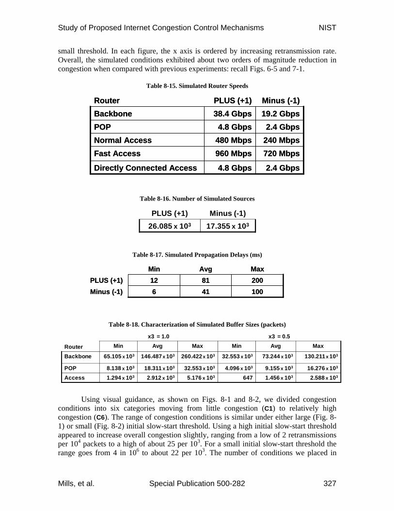
8.1.3 Domain View of Robustness Conditions Changes in network speed and network size influence the domain view of our simulated network. Table 8-15 shows the simulated router speeds for this experiment, which are about an order of magnitude below speeds that might be seen in contemporary networks. Restricting Bsources (base number of sources) to be 100 scales the number of potentially
Factor-> x1 x2 x3 x4 x5 x6 x7 x8 x9Condition -- -- -- -- -- -- -- -- --
1 -1 -1 -1 -1 -1 +1 +1 +1 +12 +1 -1 -1 -1 -1 +1 -1 -1 -13 -1 +1 -1 -1 -1 -1 +1 -1 -14 +1 +1 -1 -1 -1 -1 -1 +1 +15 -1 -1 +1 -1 -1 -1 -1 +1 -16 +1 -1 +1 -1 -1 -1 +1 -1 +17 -1 +1 +1 -1 -1 +1 -1 -1 +18 +1 +1 +1 -1 -1 +1 +1 +1 -19 -1 -1 -1 +1 -1 -1 -1 -1 +110 +1 -1 -1 +1 -1 -1 +1 +1 -111 -1 +1 -1 +1 -1 +1 -1 +1 -112 +1 +1 -1 +1 -1 +1 +1 -1 +113 -1 -1 +1 +1 -1 +1 +1 -1 -114 +1 -1 +1 +1 -1 +1 -1 +1 +115 -1 +1 +1 +1 -1 -1 +1 +1 +116 +1 +1 +1 +1 -1 -1 -1 -1 -117 -1 -1 -1 -1 +1 -1 -1 -1 -118 +1 -1 -1 -1 +1 -1 +1 +1 +119 -1 +1 -1 -1 +1 +1 -1 +1 +120 +1 +1 -1 -1 +1 +1 +1 -1 -121 -1 -1 +1 -1 +1 +1 +1 -1 +122 +1 -1 +1 -1 +1 +1 -1 +1 -123 -1 +1 +1 -1 +1 -1 +1 +1 -124 +1 +1 +1 -1 +1 -1 -1 -1 +125 -1 -1 -1 +1 +1 +1 +1 1 -126 +1 -1 -1 +1 +1 +1 -1 -1 +127 -1 +1 -1 +1 +1 -1 +1 -1 +128 +1 +1 -1 +1 +1 -1 -1 +1 -129 -1 -1 +1 +1 +1 -1 -1 +1 +130 +1 -1 +1 +1 +1 -1 +1 -1 -131 -1 +1 +1 +1 +1 +1 -1 -1 -132 +1 +1 +1 +1 +1 +1 +1 +1 +1
Study of Proposed Internet Congestion Control Mechanisms NIST
Mills, et al. Special Publication 500-282 326
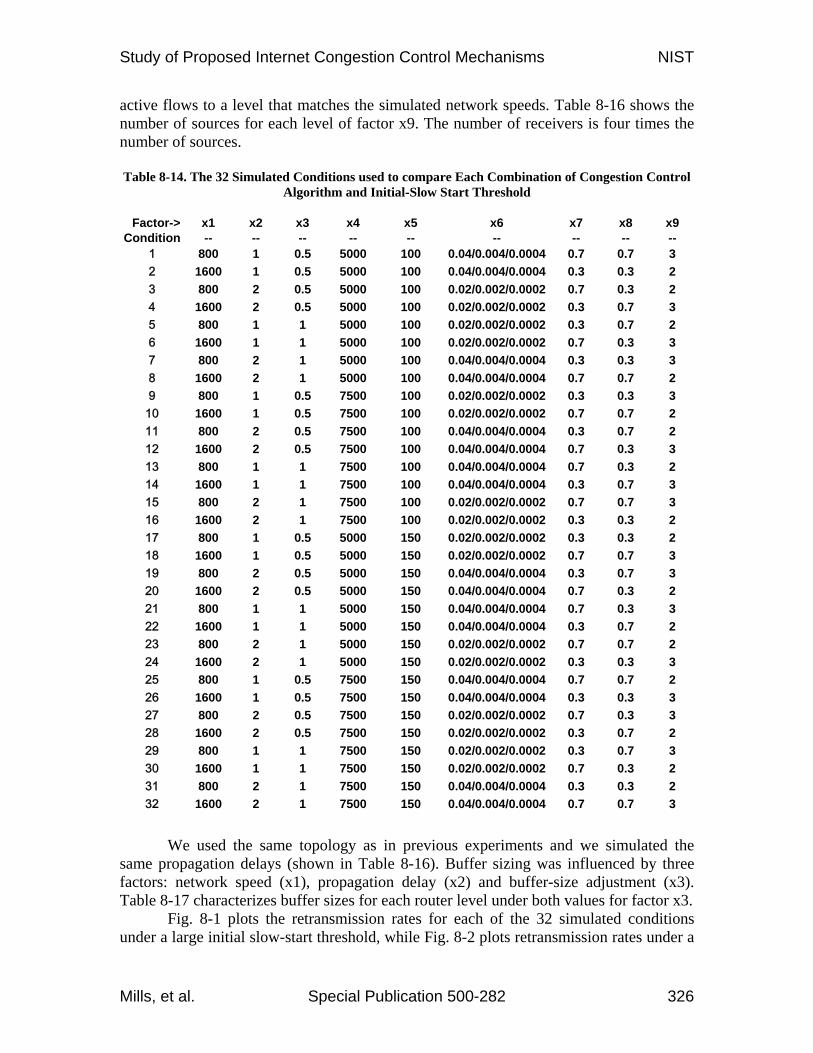
active flows to a level that matches the simulated network speeds. Table 8-16 shows the number of sources for each level of factor x9. The number of receivers is four times the number of sources. Table 8-14. The 32 Simulated Conditions used to compare Each Combination of Congestion Control
Algorithm and Initial-Slow Start Threshold
We used the same topology as in previous experiments and we simulated the same propagation delays (shown in Table 8-16). Buffer sizing was influenced by three factors: network speed (x1), propagation delay (x2) and buffer-size adjustment (x3). Table 8-17 characterizes buffer sizes for each router level under both values for factor x3.
Fig. 8-1 plots the retransmission rates for each of the 32 simulated conditions under a large initial slow-start threshold, while Fig. 8-2 plots retransmission rates under a
Factor-> x1 x2 x3 x4 x5 x6 x7 x8 x9Condition -- -- -- -- -- -- -- -- --
1 800 1 0.5 5000 100 0.04/0.004/0.0004 0.7 0.7 32 1600 1 0.5 5000 100 0.04/0.004/0.0004 0.3 0.3 23 800 2 0.5 5000 100 0.02/0.002/0.0002 0.7 0.3 24 1600 2 0.5 5000 100 0.02/0.002/0.0002 0.3 0.7 35 800 1 1 5000 100 0.02/0.002/0.0002 0.3 0.7 26 1600 1 1 5000 100 0.02/0.002/0.0002 0.7 0.3 37 800 2 1 5000 100 0.04/0.004/0.0004 0.3 0.3 38 1600 2 1 5000 100 0.04/0.004/0.0004 0.7 0.7 29 800 1 0.5 7500 100 0.02/0.002/0.0002 0.3 0.3 310 1600 1 0.5 7500 100 0.02/0.002/0.0002 0.7 0.7 211 800 2 0.5 7500 100 0.04/0.004/0.0004 0.3 0.7 212 1600 2 0.5 7500 100 0.04/0.004/0.0004 0.7 0.3 313 800 1 1 7500 100 0.04/0.004/0.0004 0.7 0.3 214 1600 1 1 7500 100 0.04/0.004/0.0004 0.3 0.7 315 800 2 1 7500 100 0.02/0.002/0.0002 0.7 0.7 316 1600 2 1 7500 100 0.02/0.002/0.0002 0.3 0.3 217 800 1 0.5 5000 150 0.02/0.002/0.0002 0.3 0.3 218 1600 1 0.5 5000 150 0.02/0.002/0.0002 0.7 0.7 319 800 2 0.5 5000 150 0.04/0.004/0.0004 0.3 0.7 320 1600 2 0.5 5000 150 0.04/0.004/0.0004 0.7 0.3 221 800 1 1 5000 150 0.04/0.004/0.0004 0.7 0.3 322 1600 1 1 5000 150 0.04/0.004/0.0004 0.3 0.7 223 800 2 1 5000 150 0.02/0.002/0.0002 0.7 0.7 224 1600 2 1 5000 150 0.02/0.002/0.0002 0.3 0.3 325 800 1 0.5 7500 150 0.04/0.004/0.0004 0.7 0.7 226 1600 1 0.5 7500 150 0.04/0.004/0.0004 0.3 0.3 327 800 2 0.5 7500 150 0.02/0.002/0.0002 0.7 0.3 328 1600 2 0.5 7500 150 0.02/0.002/0.0002 0.3 0.7 229 800 1 1 7500 150 0.02/0.002/0.0002 0.3 0.7 330 1600 1 1 7500 150 0.02/0.002/0.0002 0.7 0.3 231 800 2 1 7500 150 0.04/0.004/0.0004 0.3 0.3 232 1600 2 1 7500 150 0.04/0.004/0.0004 0.7 0.7 3
Study of Proposed Internet Congestion Control Mechanisms NIST
Mills, et al. Special Publication 500-282 327
small threshold. In each figure, the x axis is ordered by increasing retransmission rate. Overall, the simulated conditions exhibited about two orders of magnitude reduction in congestion when compared with previous experiments: recall Figs. 6-5 and 7-1.
Table 8-15. Simulated Router Speeds
Table 8-16. Number of Simulated Sources
PLUS (+1) Minus (-1)26.085 x 10³ 17.355 x 10³
Table 8-17. Simulated Propagation Delays (ms)
Table 8-18. Characterization of Simulated Buffer Sizes (packets)
Router
x3 = 1.0 x3 = 0.5Min Avg Max Min Avg Max
Backbone 65.105 x 10³ 146.487 x 10³ 260.422 x 10³ 32.553 x 10³ 73.244 x 10³ 130.211 x 10³
POP 8.138 x 10³ 18.311 x 10³ 32.553 x 10³ 4.096 x 10³ 9.155 x 10³ 16.276 x 10³
Access 1.294 x 10³ 2.912 x 10³ 5.176 x 10³ 647 1.456 x 10³ 2.588 x 10³
Using visual guidance, as shown on Figs. 8-1 and 8-2, we divided congestion
conditions into six categories moving from little congestion (C1) to relatively high congestion (C6). The range of congestion conditions is similar under either large (Fig. 8-1) or small (Fig. 8-2) initial slow-start threshold. Using a high initial slow-start threshold appeared to increase overall congestion slightly, ranging from a low of 2 retransmissions per 104 packets to a high of about 25 per 103. For a small initial slow-start threshold the range goes from 4 in 106 to about 22 per 103. The number of conditions we placed in
2.4 Gbps4.8 GbpsDirectly Connected Access
720 Mbps960 MbpsFast Access240 Mbps480 MbpsNormal Access2.4 Gbps4.8 GbpsPOP
19.2 Gbps38.4 GbpsBackboneMinus (-1)PLUS (+1)Router
2.4 Gbps4.8 GbpsDirectly Connected Access
720 Mbps960 MbpsFast Access240 Mbps480 MbpsNormal Access2.4 Gbps4.8 GbpsPOP
19.2 Gbps38.4 GbpsBackboneMinus (-1)PLUS (+1)Router
100416Minus (-1)2008112PLUS (+1)MaxAvgMin
100416Minus (-1)2008112PLUS (+1)MaxAvgMin

Study of Proposed Internet Congestion Control Mechanisms NIST
Mills, et al. Special Publication 500-282 328
particular categories varies slightly between the two figures. In addition, the order of the conditions varies somewhat between the two figures. Eight conditions changed categories when moving from a large to a small initial slow-start threshold. Seven of those conditions moved to a less congested category. Overall, however, the relative congestion generated by the same condition under either of the two initial slow-start thresholds appears similar.
Figure 8-1. Conditions Ordered from Least to Most Congested (High Initial Slow-Start Threshold)
Figure 8-2. Conditions Ordered from Least to Most Congested (Low Initial Slow-Start Threshold)
0
0.005
0.01
0.015
0.02
0.025
0.03
16 8 24 32 28 12 4 20 14 6 30 22 15 2 10 31 23 26 11 3 7 13 5 18 27 9 29 25 17 1 19 21
Condition
Ret
rans
mis
sion
Rat
e
Min = 2 in 10,000 Max = 2.5 in 100C1 C2 C3 C4 C5 C6
0
0.005
0.01
0.015
0.02
0.025
0.03
16 8 24 32 28 12 4 20 14 6 30 22 15 2 10 31 23 26 11 3 7 13 5 18 27 9 29 25 17 1 19 21
Condition
Ret
rans
mis
sion
Rat
e
Min = 2 in 10,000 Max = 2.5 in 100C1 C2 C3 C4 C5 C6
0.000
0.005
0.010
0.015
0.020
0.025
0.030
16 8 24 12 32 28 4 14 30 20 6 22 15 2 10 31 23 11 3 26 7 13 5 18 27 9 29 25 17 1 19 21
Condition
Retra
nsm
issi
on R
ate
Min = 4 in 1,0000,000 Max = 2.2 in 100C1 C2 C3 C4 C5 C6
0.000
0.005
0.010
0.015
0.020
0.025
0.030
16 8 24 12 32 28 4 14 30 20 6 22 15 2 10 31 23 11 3 26 7 13 5 18 27 9 29 25 17 1 19 21
Condition
Retra
nsm
issi
on R
ate
Min = 4 in 1,0000,000 Max = 2.2 in 100C1 C2 C3 C4 C5 C6
Study of Proposed Internet Congestion Control Mechanisms NIST
Mills, et al. Special Publication 500-282 329
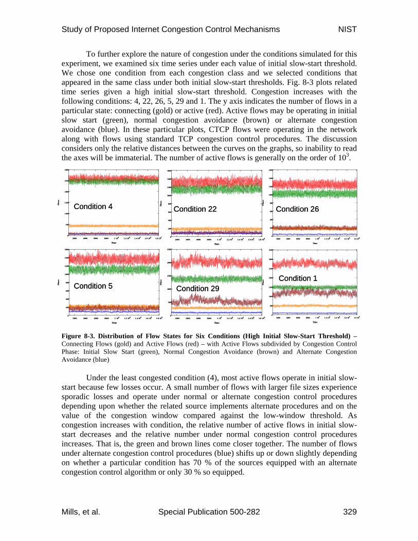
To further explore the nature of congestion under the conditions simulated for this experiment, we examined six time series under each value of initial slow-start threshold. We chose one condition from each congestion class and we selected conditions that appeared in the same class under both initial slow-start thresholds. Fig. 8-3 plots related time series given a high initial slow-start threshold. Congestion increases with the following conditions: 4, 22, 26, 5, 29 and 1. The y axis indicates the number of flows in a particular state: connecting (gold) or active (red). Active flows may be operating in initial slow start (green), normal congestion avoidance (brown) or alternate congestion avoidance (blue). In these particular plots, CTCP flows were operating in the network along with flows using standard TCP congestion control procedures. The discussion considers only the relative distances between the curves on the graphs, so inability to read the axes will be immaterial. The number of active flows is generally on the order of 103. Figure 8-3. Distribution of Flow States for Six Conditions (High Initial Slow-Start Threshold) – Connecting Flows (gold) and Active Flows (red) – with Active Flows subdivided by Congestion Control Phase: Initial Slow Start (green), Normal Congestion Avoidance (brown) and Alternate Congestion Avoidance (blue)
Under the least congested condition (4), most active flows operate in initial slow-start because few losses occur. A small number of flows with larger file sizes experience sporadic losses and operate under normal or alternate congestion control procedures depending upon whether the related source implements alternate procedures and on the value of the congestion window compared against the low-window threshold. As congestion increases with condition, the relative number of active flows in initial slow-start decreases and the relative number under normal congestion control procedures increases. That is, the green and brown lines come closer together. The number of flows under alternate congestion control procedures (blue) shifts up or down slightly depending on whether a particular condition has 70 % of the sources equipped with an alternate congestion control algorithm or only 30 % so equipped.
2000 4000 6000 8000 1 .104 1.2 .104 1.4 .104 1.6 .104 1.8 .1040
500
1000
1500
2000
2500
Time
Flow
s
2000 4000 6000 8000 1 .104 1.2 .104 1.4 .104 1.6 .104 1.8 .1040
500
1000
1500
2000
2500
3000
Time
Flow
s
2000 4000 6000 8000 1 .104 1.2 .104 1.4 .104 1.6 .104 1.8 .1040
200
400
600
800
1000
1200
1400
1600
Time
Flow
s
Condition 4 Condition 22
2000 4000 6000 8000 1 .104 1.2 .104 1.4 .104 1.6 .104 1.8 .1040
200
400
600
800
1000
1200
1400
1600
Time
Flow
s
Condition 26
2000 4000 6000 8000 1 .104 1.2 .104 1.4 .104 1.6 .104 1.8 .1040
200
400
600
800
1000
1200
1400
1600
Time
Flow
s
Condition 5
2000 4000 6000 8000 1 .104 1.2 .104 1.4 .104 1.6 .104 1.8 .1040
500
1000
1500
2000
2500
3000
3500
Time
Flow
s Condition 1Condition 29
2000 4000 6000 8000 1 .104 1.2 .104 1.4 .104 1.6 .104 1.8 .1040
500
1000
1500
2000
2500
Time
Flow
s
2000 4000 6000 8000 1 .104 1.2 .104 1.4 .104 1.6 .104 1.8 .1040
500
1000
1500
2000
2500
3000
Time
Flow
s
2000 4000 6000 8000 1 .104 1.2 .104 1.4 .104 1.6 .104 1.8 .1040
200
400
600
800
1000
1200
1400
1600
Time
Flow
s
Condition 4 Condition 22
2000 4000 6000 8000 1 .104 1.2 .104 1.4 .104 1.6 .104 1.8 .1040
200
400
600
800
1000
1200
1400
1600
Time
Flow
s
Condition 26
2000 4000 6000 8000 1 .104 1.2 .104 1.4 .104 1.6 .104 1.8 .1040
200
400
600
800
1000
1200
1400
1600
Time
Flow
s
Condition 5
2000 4000 6000 8000 1 .104 1.2 .104 1.4 .104 1.6 .104 1.8 .1040
500
1000
1500
2000
2500
3000
3500
Time
Flow
s Condition 1Condition 29

Study of Proposed Internet Congestion Control Mechanisms NIST
Mills, et al. Special Publication 500-282 330
Fig. 8-4 plots the same conditions as Fig. 8-3 but under a small initial slow-start threshold. Comparison of the figures reveals the fundamental influence of the value of initial slow-start threshold on the distribution of flow states. First, note that except for the most highly congested condition relatively fewer flows operate in initial slow-start. This stands to reason because flows must transition from initial slow-start once the threshold is reached, so relatively more flows will move to alternate or normal congestion avoidance mode. As congestion increases, the proportion of flows in initial slow-start converges with the proportion of flows in normal congestion control mode. The proportion of flows under alternate congestion control procedures shifts up or down slightly depending on whether a particular condition has more or fewer sources equipped with alternate congestion control procedures. This comparison further demonstrates that the same conditions produce similar congestion patterns no matter whether the initial slow-start threshold is large or small. Figure 8-4. Distribution of Flow States for Six Conditions (Low Initial Slow-Start Threshold) – Connecting Flows (gold) and Active Flows (red) – with Active Flows subdivided by Congestion Control Phase: Initial Slow Start (green), Normal Congestion Avoidance (brown) and Alternate Congestion Avoidance (blue)
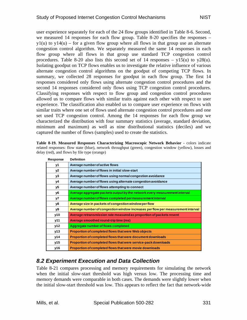
8.1.4 Responses Measured As in previous experiments we measured responses in two categories: macroscopic behavior of the network and user experience. In the current experiment, however, we selected somewhat different responses in each category. Table 8-19 enumerates responses (y1 to y16) characterizing macroscopic behavior. We grouped the 16 responses into five subsets (color coded in Table 8-19) measuring: number of flows in a given state (blue); network-wide throughput in packets and flows (green); congestion window size and dynamics (yellow); congestion and delay (red); and proportion of completed flows by file type (orange). We used these responses to assess whether adopting a particular alternate congestion control algorithm alters global behavior in the simulated network.
Measuring user experience for the current experiment became more complicated than was the case for earlier experiments. First, in the current experiment we measured
2000 4000 6000 8000 1 .104 1.2 .104 1.4 .104 1.6 .104 1.8 .1040
500
1000
1500
2000
2500
3000
3500
Time
Flow
s
2000 4000 6000 8000 1 .104 1.2 .104 1.4 .104 1.6 .104 1.8 .1040
500
1000
1500
2000
2500
Time
Flow
s
2000 4000 6000 8000 1 .104 1.2 .104 1.4 .104 1.6 .104 1.8 .1040
200
400
600
800
1000
1200
1400
1600
Time
Flow
s
CTCP Condition 4 CTCP Condition 22 CTCP Condition 26
CTCP Condition 5
CTCP Condition 1
2000 4000 6000 8000 1 .104 1.2 .104 1.4 .104 1.6 .104 1.8 .1040
500
1000
1500
2000
2500
3000
Time
Flow
s
CTCP Condition 29
2000 4000 6000 8000 1 .104 1.2 .104 1.4 .104 1.6 .104 1.8 .1040
200
400
600
800
1000
1200
1400
1600
Time
Flow
s
2000 4000 6000 8000 1 .104 1.2 .104 1.4 .104 1.6 .104 1.8 .1040
200
400
600
800
1000
1200
1400
1600
TimeFl
ows
2000 4000 6000 8000 1 .104 1.2 .104 1.4 .104 1.6 .104 1.8 .1040
500
1000
1500
2000
2500
3000
3500
Time
Flow
s
2000 4000 6000 8000 1 .104 1.2 .104 1.4 .104 1.6 .104 1.8 .1040
500
1000
1500
2000
2500
Time
Flow
s
2000 4000 6000 8000 1 .104 1.2 .104 1.4 .104 1.6 .104 1.8 .1040
200
400
600
800
1000
1200
1400
1600
Time
Flow
s
CTCP Condition 4 CTCP Condition 22 CTCP Condition 26
CTCP Condition 5
CTCP Condition 1
2000 4000 6000 8000 1 .104 1.2 .104 1.4 .104 1.6 .104 1.8 .1040
500
1000
1500
2000
2500
3000
Time
Flow
s
CTCP Condition 29
2000 4000 6000 8000 1 .104 1.2 .104 1.4 .104 1.6 .104 1.8 .1040
200
400
600
800
1000
1200
1400
1600
Time
Flow
s
2000 4000 6000 8000 1 .104 1.2 .104 1.4 .104 1.6 .104 1.8 .1040
200
400
600
800
1000
1200
1400
1600
TimeFl
ows
Study of Proposed Internet Congestion Control Mechanisms NIST
Mills, et al. Special Publication 500-282 331
user experience separately for each of the 24 flow groups identified in Table 8-6. Second, we measured 14 responses for each flow group. Table 8-20 specifies the responses – y1(u) to y14(u) – for a given flow group where all flows in that group use an alternate congestion control algorithm. We separately measured the same 14 responses in each flow group where all flows in that group use standard TCP congestion control procedures. Table 8-20 also lists this second set of 14 responses – y15(u) to y28(u). Isolating goodput on TCP flows enables us to investigate the relative influence of various alternate congestion control algorithms on the goodput of competing TCP flows. In summary, we collected 28 responses for goodput in each flow group. The first 14 responses considered only flows using alternate congestion control procedures and the second 14 responses considered only flows using TCP congestion control procedures. Classifying responses with respect to flow group and congestion control procedures allowed us to compare flows with similar traits against each other with respect to user experience. The classification also enabled us to compare user experience on flows with similar traits where one set of flows used alternate congestion control procedures and one set used TCP congestion control. Among the 14 responses for each flow group we characterized the distribution with four summary statistics (average, standard deviation, minimum and maximum) as well as nine distributional statistics (deciles) and we captured the number of flows (samples) used to create the statistics. Table 8-19. Measured Responses Characterizing Macroscopic Network Behavior - colors indicate related responses: flow state (blue), network throughput (green), congestion window (yellow), losses and delay (red), and flows by file type (orange)
Response Definitiony1 Average number of active flowsy2 Average number of flows in initial slow-starty3 Average number of flows using normal congestion avoidancey4 Average number of flows using alternate congestion avoidancey5 Average number of flows attempting to connecty6 Average aggregate packets output by the network every measurement intervaly7 Average number of flows completed per measurement intervaly8 Average size in packets of congestion window per flowy9 Average number of congestion window increases per flow per measurement interval
y10 Average retransmission rate measured as proportion of packets resenty11 Average smoothed round-trip time (ms)y12 Aggregate number of flows completedy13 Proportion of completed flows that were Web objectsy14 Proportion of completed flows that were document downloadsy15 Proportion of completed flows that were service-pack downloadsy16 Proportion of completed flows that were movie downloads
8.2 Experiment Execution and Data Collection Table 8-21 compares processing and memory requirements for simulating the network when the initial slow-start threshold was high versus low. The processing time and memory demands were comparable in both cases. The demands were slightly lower when the initial slow-start threshold was low. This appears to reflect the fact that network-wide

Study of Proposed Internet Congestion Control Mechanisms NIST
Mills, et al. Special Publication 500-282 332
congestion was somewhat lower when the initial slow-start threshold was not extremely high. Table 8-22 gives evidence corroborating this hypothesis. Notice that about 7 million more flows were completed in the 224 simulated hours (about 30 x 103 flows per hour) when the initial slow-start threshold was set low. Also notice that completing those flows required about 42 billion fewer packets. This result is consistent with lower congestion when the initial slow-start threshold was set to the lower value. Table 8-20. Measured Responses Characterizing User Experience for Each Flow Group, inlcuding Flows using an Alternate Congestion Control Algorithm, y1(u) – y14(u), and Competing TCP Flows, y15(u) – y18(u)
90th Percentile in goodputy14(u)80th Percentile in goodputy13(u)70th Percentile in goodputy12(u)60th Percentile in goodputy11(u)50th Percentile in goodputy10(u)40th Percentile in goodputy9(u)30th Percentile in goodputy8(u)20th Percentile in goodputy7(u)10th Percentile in goodputy6(u)Maximum goodputy5(u)Minimum goodputy4(u)Standard deviation in goodputy3(u)Average goodputy2(u)
Total number of flows in group that used alternate congestion avoidance
y1(u)
DefinitionResponse
90th Percentile in goodputy28(u)80th Percentile in goodputy27(u)70th Percentile in goodputy26(u)60th Percentile in goodputy25(u)50th Percentile in goodputy24(u)40th Percentile in goodputy23(u)30th Percentile in goodputy22(u)20th Percentile in goodputy21(u)10th Percentile in goodputy20(u)Maximum goodputy19(u)Minimum goodputy18(u)Standard deviation in goodputy17(u)Average goodputy16(u)
Total number of flows in group that used standard TCP congestion avoidance
y15(u)

Study of Proposed Internet Congestion Control Mechanisms NIST
Mills, et al. Special Publication 500-282 333
8.2.1 Computing Macroscopic Responses We computed macroscopic responses in two general forms. In one form we counted events for each run over the simulated period (one hour). Specifically, for responses y12 through y16 we counted the number of completed flows and categorized each completed flow by file type. Then we computed the proportion of completed files by type (y13 to y16) as the ratio of the count by type to total flows completed. Table 8-21. Comparing Resource Requirements for Simulating One Hour of Network Operation under 32 Conditions with High and Low Initial Slow-Start Thresholds
Small Network with High Initial Slow-Start
Threshold
Small Network with Low Initial Slow-Start
ThresholdCPU hours (224 Runs) 5.857 x 10³ 5.639 x 10³
Avg. CPU hours(per run) 26.15 25.17
Min. CPU hours(one run) 12.58 12.51
Max. CPU hours(one run) 43.97 40.94
Avg. Memory Usage (Mbytes) 196.56 194.46
Table 8-22. Comparing Flows Completed and Data Packets Sent when Simulating One Hour of Network Operation under 32 Conditions with High and Low Initial Slow-Start Thresholds
Small Network with High Initial Slow-Start Threshold
Small Network with Low Initial Slow-Start Threshold
Statistic Flows Completed Data Packets Sent Flows Completed Data Packets Sent
Avg. Per Condition 11.466 x 10⁶ 3.414 x 10⁹ 11.495 x 10⁶ 3.225 x 10⁹
Min. Per Condition 7.258 x 10⁶ 2.139 x 10⁹ 7.263 x 10⁶ 2.055 x 10⁹
Max. Per Condition 17.391 x 10⁶ 5.048 x 10⁹ 17.432 x 10⁶ 4.832 x 10⁹
Total all Runs 2.568 x 10⁹ 764,740 x 109 2.575 x 10⁹ 722.466 x 10⁹
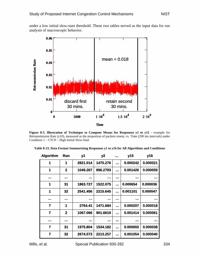
For each of the responses y1 through y11 we computed average values from a time series of 9000 measurements. Figure 8-5 illustrates an example of such a computation for response y10, average retransmission rate. This example was taken from simulated condition 1 in the case where CTCP was the alternate congestion control algorithm and where the initial slow-start threshold was high. Notice that we discarded the first half of the time series, which avoided startup transients. We computed the mean of the second half of the time series; in this case the mean retransmission rate was 0.018.
We organized all responses measuring macroscopic network behavior into a table, where each row contained the 16 responses under a given condition and alternate congestion control algorithm. Table 8-23 depicts the response format in the case when the initial slow-start threshold is high. We created a similar table for responses obtained
Study of Proposed Internet Congestion Control Mechanisms NIST
Mills, et al. Special Publication 500-282 334
under a low initial slow-start threshold. These two tables served as the input data for our analysis of macroscopic behavior. Figure 8-5. Illustration of Technique to Compute Means for Responses y1 to y11 - example for Retransmission Rate (y10), measured as the proportion of packets resent, vs. Time (200 ms intervals) under Condition 1 – CTCP – High Initial Slow-Start
Table 8-23. Data Format Summarizing Responses y1 to y16 for All Algorithms and Conditions
0 5000 1 .104 1.5 .104 2 .1040
0.01
0.02
0.03
0.04
0.05
0.06
Time
Ret
rans
mis
sion
Rate
discard first30 mins.
retain second30 mins.
mean = 0.018
0 5000 1 .104 1.5 .104 2 .1040
0.01
0.02
0.03
0.04
0.05
0.06
Time
Ret
rans
mis
sion
Rate
discard first30 mins.
retain second30 mins.
mean = 0.018
…………………
0.0000380.000650…1534.1821975.804317
0.0000400.001054…2213.2572674.573327
0.0000610.001414…901.66191067.06627
0.0000180.000207…1471.6842764.4117
…………………
0.0000470.001101…2215.6452541.456321
0.0000360.000654…1522.0751863.727311
…………………
0.0000590.001426…896.27931049.26721
0.0000210.000242…1475.2762821.01411
y16y15…y2y1RunAlgorithm
…………………
0.0000380.000650…1534.1821975.804317
0.0000400.001054…2213.2572674.573327
0.0000610.001414…901.66191067.06627
0.0000180.000207…1471.6842764.4117
…………………
0.0000470.001101…2215.6452541.456321
0.0000360.000654…1522.0751863.727311
…………………
0.0000590.001426…896.27931049.26721
0.0000210.000242…1475.2762821.01411
y16y15…y2y1RunAlgorithm
Study of Proposed Internet Congestion Control Mechanisms NIST
Mills, et al. Special Publication 500-282 335
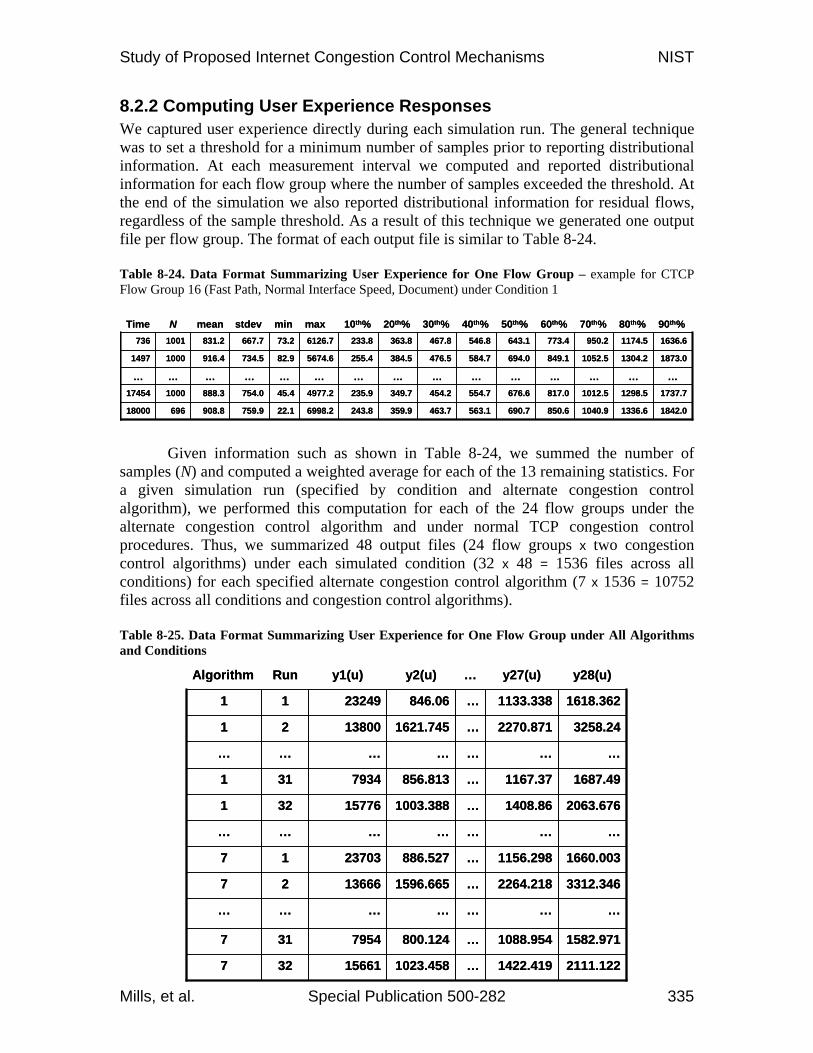
8.2.2 Computing User Experience Responses We captured user experience directly during each simulation run. The general technique was to set a threshold for a minimum number of samples prior to reporting distributional information. At each measurement interval we computed and reported distributional information for each flow group where the number of samples exceeded the threshold. At the end of the simulation we also reported distributional information for residual flows, regardless of the sample threshold. As a result of this technique we generated one output file per flow group. The format of each output file is similar to Table 8-24. Table 8-24. Data Format Summarizing User Experience for One Flow Group – example for CTCP Flow Group 16 (Fast Path, Normal Interface Speed, Document) under Condition 1
Given information such as shown in Table 8-24, we summed the number of samples (N) and computed a weighted average for each of the 13 remaining statistics. For a given simulation run (specified by condition and alternate congestion control algorithm), we performed this computation for each of the 24 flow groups under the alternate congestion control algorithm and under normal TCP congestion control procedures. Thus, we summarized 48 output files (24 flow groups x two congestion control algorithms) under each simulated condition (32 x 48 = 1536 files across all conditions) for each specified alternate congestion control algorithm (7 x 1536 = 10752 files across all conditions and congestion control algorithms). Table 8-25. Data Format Summarizing User Experience for One Flow Group under All Algorithms and Conditions
850.6
817.0
…
849.1
773.4
60th%
1040.9
1012.5
…
1052.5
950.2
70th%
1336.6
1298.5
…
1304.2
1174.5
80th%
1842.0690.7563.1463.7359.9243.86998.222.1759.9908.869618000
1737.7676.6554.7454.2349.7235.94977.245.4754.0888.3100017454
………………………………
1873.0694.0584.7476.5384.5255.45674.682.9734.5916.410001497
1636.6643.1546.8467.8363.8233.86126.773.2667.7831.21001736
90th%50th%40th%30th%20th%10th%maxminstdevmeanNTime
…………………
1582.9711088.954…800.1247954317
2111.1221422.419…1023.45815661327
3312.3462264.218…1596.6651366627
1660.0031156.298…886.5272370317
…………………
2063.6761408.86…1003.38815776321
1687.491167.37…856.8137934311
…………………
3258.242270.871…1621.7451380021
1618.3621133.338…846.062324911
y28(u)y27(u)…y2(u)y1(u)RunAlgorithm
…………………
1582.9711088.954…800.1247954317
2111.1221422.419…1023.45815661327
3312.3462264.218…1596.6651366627
1660.0031156.298…886.5272370317
…………………
2063.6761408.86…1003.38815776321
1687.491167.37…856.8137934311
…………………
3258.242270.871…1621.7451380021
1618.3621133.338…846.062324911
y28(u)y27(u)…y2(u)y1(u)RunAlgorithm
Study of Proposed Internet Congestion Control Mechanisms NIST
Mills, et al. Special Publication 500-282 336
For a given flow group, we concatenated the 14 responses on flows using alternate congestion control together with the 14 responses on flows using TCP congestion control and appended identifiers for the alternate algorithm and the condition to produce a 30 cell row for each combination, as illustrated in Table 8-25. Thus, we summarized user-experience responses into 24 files: one per flow group. Where needed to make data analysis more convenient, we concatenated all flow groups into a single file, adding a cell to each row to identify the flow group associated with the data. A single concatenated file contained (24 x 7 x 32 =) 5376 rows, one for each combination of flow group, alternate congestion control algorithm and simulated condition.
8.3 Data Analysis Approach Most of the data analyses conducted for this experiment focused on user experience. Before explaining the techniques we applied to analyze user experience, we provide a brief summary of the single technique we applied to analyze macroscopic responses.
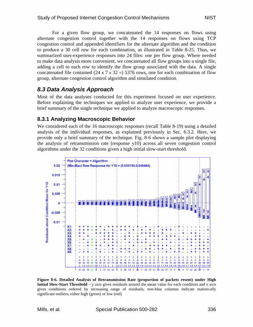
8.3.1 Analyzing Macroscopic Behavior We considered each of the 16 macroscopic responses (recall Table 8-19) using a detailed analysis of the individual responses, as explained previously in Sec. 6.3.2. Here, we provide only a brief summary of the technique. Fig. 8-6 shows a sample plot displaying the analysis of retransmission rate (response y10) across all seven congestion control algorithms under the 32 conditions given a high initial slow-start threshold. Figure 8-6. Detailed Analysis of Retransmission Rate (proportion of packets resent) under High Initial Slow-Start Threshold – y axis gives residuals around the mean value for each condition and x axis gives conditions ordered by increasing range of residuals; non-blue columns indicate statistically significant outliers, either high (green) or low (red)
Study of Proposed Internet Congestion Control Mechanisms NIST
Mills, et al. Special Publication 500-282 337
For each condition, we computed the mean response and then reformulated the response for each algorithm as residuals around the condition mean by subtracting the response from the condition mean. We then sorted the conditions from the least to greatest extreme (by magnitude of the) residual and plotted the residuals (y axis) along with the factor settings associated with the related conditions (x axis). Below the factor settings we identified the algorithm exhibiting the most extreme residual. We also indicated the order of magnitude and percentage difference in the extreme residual from the mean. We applied a Grubbs’ test to determine if the extreme residual represented a statistically significant difference from the mean. If the difference was statistically significant on the positive side, then we colored the column green. If significant on the negative side, we colored the column red. Otherwise, the column remains blue.
8.3.2 Analyzing User Experience We analyzed user experience with respect to the 24 flow classes identified in Table 8-6. In each class, we considered the experience of normal TCP users and also the experience of users under a competing alternate congestion control algorithm. We measured user experience as goodput (i.e., packets received per unit of time, excluding retransmissions). While we collected distributional data for each flow group (recall Table 8-20), the analyses described in this section focus solely on mean goodput for users under alternate congestion control – y2(u) – and under standard TCP congestion control – y16(u).
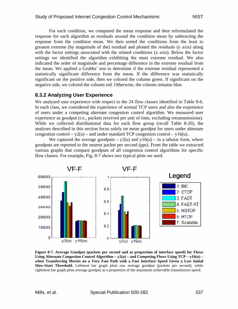
We captured the average goodputs – y2(u) and y16(u) – in a tabular form, where goodputs are reported to the nearest packet per second (pps). From the table we extracted various graphs that compare goodputs of all congestion control algorithms for specific flow classes. For example, Fig. 8-7 shows two typical plots we used. Figure 8-7. Average Goodput (packets per second and as proportion of interface speed) for Flows Using Alternate Congestion Control Algorithm – y2(u) – and Competing Flows Using TCP – y16(u) – when Transferring Movies on a Very Fast Path with a Fast Interface Speed Given a Low Initial Slow-Start Threshold. Leftmost bar graph plots raw average goodput (packets per second), while rightmost bar graph plots average goodput as a proportion of the maximum achievable transmission speed.
VF-FLegend
VF-FVF-FVF-FLegendLegend
VF-FVF-F

Study of Proposed Internet Congestion Control Mechanisms NIST
Mills, et al. Special Publication 500-282 338
The legend in Fig. 8-7 shows the bar color associated with a particular alternate congestion control algorithm. When plotted in bar graphs we plot the algorithms by increasing identifier from 1 (BIC) to 7 (Scalable). Each bar graph is labeled with the path class (VF in Fig. 8-7) and interface speed (F in Fig. 8-7). The bar graphs in Fig. 8-7 plot average goodput when transferring movies over very fast paths with a fast interface speed (maximum of 80 x 103 pps) given a low initial slow-start threshold. The leftmost graph gives the raw average goodput (y axis) for each congestion control algorithm (one bar each). The first set of seven bars represents the goodput achieved on flows using a specific alternate congestion control algorithm. The second set of seven bars represents goodput achieved on flows using normal TCP congestion control but operating in a network where some flows use a specified, competing alternate congestion control algorithm. The rightmost graph is formulated in the same fashion except that the y axis expresses goodput as a fraction of the maximum achievable transfer rate (80 x 103 pps here). The leftmost graph illustrates differences in goodput among the various algorithms and also identifies differences in goodput between the alternate algorithms and normal TCP. The rightmost graph shows the degree to which the various flows were able to achieve the maximum available goodputs.
To investigate causes of variation in goodputs, we employed principal components analyses (PCA) on the average goodput data – y2(u) and y16(u) – for each of the seven alternative congestion control algorithms under all 32 conditions. For each given algorithm a and condition c we collected 24 observations for y2(u) (one per flow group) and 24 for y16(u) (one per flow group) into a 48-dimension vector: (x1, x2, …, x48)a,c for a total of (32 x 7 =) 224 vector instances. We then conducted a PCA, as described earlier in Sec. 4.5, which yielded plots such as shown in Fig. 8-8. Figure 8-8. Principal Components Analysis of Goodputs given High Slow-Start Threshold – three subplots give the weight vectors for the first three PCs and one bargraph indicates the proportion of variance explained by each of the first three PCs, as well as the variance explained by a combination of the first three PCs

Study of Proposed Internet Congestion Control Mechanisms NIST
Mills, et al. Special Publication 500-282 339
As Fig. 8-8 demonstrates nearly all variation in the data could be accounted for by the first three principal components (PC). We plotted pairs of PCs against one another in biplots to investigate whether specific factors caused similarity among goodputs. Fig. 8-9 gives an example of one such plot of PC1 (x axis) vs. PC 2 (y axis). The legend associates each congestion control algorithm with a particular colored symbol. Fig. 8-9 clearly shows three groups of observations (circled). Two of the groups divide into two subgroups. As explained below in Sec. 8.4.2, we analyzed factors in common among observations in each group to provide information about the causes of these groupings.
PC
2
PC1
LegendBICCTCPFAST
FAST-ATHSTCP
HTCPSCALABLE
Figure 8-9. Illustration of Biplot of PC1 vs. PC2 and Related Clustering
To compare goodputs provided on normal TCP flows against goodputs provided on flows using alternate congestion control algorithms, we adopted two main techniques. First, we created plots of y2(u) vs. y16(u) for all 32 conditions for a given flow group and alternate congestion control algorithm. For example, Fig. 8-10 shows such a plot for algorithm 3 (FAST) when transferring movies over very fast paths with a fast interface speed given a high initial slow-start threshold. The figure in red (0.96632) above the plot is the computed correlation between y2(u) and y16(u). Points below the diagonal indicate cases where flows using the alternate congestion control regime achieved higher average goodput, while points above the diagonal indicate cases where TCP flows achieved higher average goodput. A strong positive correlation indicates that the trend in goodputs for all flows was linear with respect to condition.
As a second technique to compare goodput of TCP flows vs. goodput of flows using alternate congestion control algorithms, we plotted bar graphs for each condition and flow group, where each bar spans two points for each algorithm. One point represents y2(u)/1000 and one represents y16(u)/1000. If the y2(u) value is higher, then the bar is colored green. If the y16(u) value is higher, the bar is colored red. Fig. 8-11 shows a sample of such a bar graph. The bar for algorithm 4 (FAST-AT) is colored red, which shows that for this condition and flow group TCP flows achieved about 5000 pps higher

Study of Proposed Internet Congestion Control Mechanisms NIST
Mills, et al. Special Publication 500-282 340
(40 p/ms – 35 p/ms = 5 p/ms) average goodput than FAST-AT flows. The specific condition (21; most congested) is reported in the lower left corner of the plot. Figure 8-10. Scatter Plot of y16(u)/100 vs. y2(u)/100 for Movies Transferred over a Very Fast Path with Fast Interface Speed Given a High Initial Slow-Start Threshold; FAST Alternate Congestion Control Algorithm Figure 8-11. Bar Graph for Movies Transferred over a Very Fast Path with Fast Interface Speed given a High Initial Slow-Start Threshold during Condition 21 (Most Congested) – each bar is formed by plotting y16(u)/1000 and y2(u)/1000 for a Specific Alternate Congestion Control Algorithm (plotted from 1 to 7 left to right) – if a bar is red then y16(u)/1000 is plotted at the top of the bar and y2(u)/1000 is plotted at the bottom of the bar; otherwise (green bar) y2(u)/1000 is plotted at the top of the bar and y16(u)/1000 is plotted at the bottom of the bar – y axis gives goodput (packets/ms)
In addition to analyzing absolute differences in goodput among the alternate congestion control algorithms and between the alternates and normal TCP congestion control, we also analyzed the relative differences. To compare relative differences we adopted a rank analysis. For each given flow group and condition we compared the y2(u)
Study of Proposed Internet Congestion Control Mechanisms NIST
Mills, et al. Special Publication 500-282 341
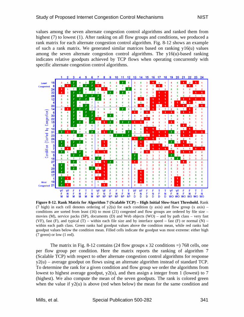
values among the seven alternate congestion control algorithms and ranked them from highest (7) to lowest (1). After ranking on all flow groups and conditions, we produced a rank matrix for each alternate congestion control algorithm. Fig. 8-12 shows an example of such a rank matrix. We generated similar matrices based on ranking y16(u) values among the seven alternate congestion control algorithms. The y16(u)-based ranking indicates relative goodputs achieved by TCP flows when operating concurrently with specific alternate congestion control algorithms.
Figure 8-12. Rank Matrix for Algorithm 7 (Scalable TCP) – High Initial Slow-Start Threshold. Rank (7 high) in each cell denotes ordering of y2(u) for each condition (y axis) and flow group (x axis) – conditions are sorted from least (16) to most (21) congested and flow groups are ordered by file size – movies (M), service packs (SP), documents (D) and Web objects (WO) – and by path class – very fast (VF), fast (F), and typical (T) – within each file size and by interface speed – fast (F) or normal (N) – within each path class. Green ranks had goodput values above the condition mean, while red ranks had goodput values below the condition mean. Filled cells indicate the goodput was most extreme: either high (7 green) or low (1 red).
The matrix in Fig. 8-12 contains (24 flow groups x 32 conditions =) 768 cells, one per flow group per condition. Here the matrix reports the ranking of algorithm 7 (Scalable TCP) with respect to other alternate congestion control algorithms for response y2(u) – average goodput on flows using an alternate algorithm instead of standard TCP. To determine the rank for a given condition and flow group we order the algorithms from lowest to highest average goodput, y2(u), and then assign a integer from 1 (lowest) to 7 (highest). We also compute the mean of the seven goodputs. The rank is colored green when the value if y2(u) is above (red when below) the mean for the same condition and
Study of Proposed Internet Congestion Control Mechanisms NIST
Mills, et al. Special Publication 500-282 342
flow group. If the value of y2(u) is most distance from the mean the rank is filled – green for highest (7) and red for lowest (1). A quick glance at Fig. 8-12 reveals that Scalable TCP appears to provide best goodput for larger files (movies and service packs) and worst goodput for smaller files (documents and Web objects). Given a complete set of 14 matrices, one per algorithm ranking y2(u) values and one per algorithm ranking y16(u) values, we also computed the average (and standard deviation) of the ranking for each algorithm with respect to each file type. The resulting tables (Tables 8-31 and 8-32) allowed us to succinctly compare relative ranking among the algorithms.
8.4 Results Here, we present selected simulation results in three categories: (1) macroscopic network behavior, (2) absolute user experience and (3) relative user experience. Within each category, we first give relevant data under a high initial slow-start threshold followed by data under a low initial slow-start threshold. We present only data that reveals behavioral similarities and differences of interest.
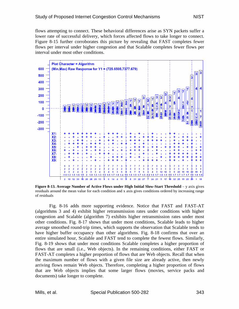
8.4.1 Macroscopic Network Behavior In general, the data analyses reported in this section do not reveal much in the way of statistically significant changes in macroscopic network behavior. This appears due mainly to a general lack of congestion throughout these experiments. In addition, we consider both FAST (algorithm 3) and FAST-AT (algorithm 4) together in these analyses, which reduces the statistical significance of either algorithm considered alone because both algorithms share some traits (as described previously in Chapter 7). Despite this, we could discern patterns in macroscopic network behavior with respect to some responses. In most cases, the patterns detected echo patterns seen in previous experiments, where simulated congestion tended to be much higher under most conditions. Here, we report the patterns we found informative. 8.4.1.1 High Initial Slow-start Threshold. Fig. 8-13 gives a detailed analysis of the average number of active flows under the 32 simulated conditions. Notice that in most conditions either algorithm 7 (Scalable TCP) or 3 (FAST) shows a higher number of active flows than other algorithms. This suggests that these algorithms have some number of flows that take longer to complete. Algorithm 3 exhibits the extreme value under conditions with highest congestion. This suggests that under those conditions, some FAST flows exhibit the oscillatory behavior identified in previous experiments (recall Chapter 6), which induces excessive losses and lowers goodput on affected flows. In previous experiments (see Chapter 5), Scalable TCP was found to provide significant unfairness when new flows attempt to gain bandwidth from already established flows. This occurs because Scalable TCP flows occupy significant buffer space and reduce their congestion window little on each loss, which causes affected new flows to experience a larger proportion of losses, and lower goodputs. The reader should keep these ideas in mind as additional responses are presented.
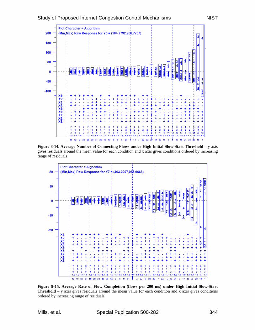
Fig. 8-14, which shows the average number of flows attempting to connect, supports the analysis from the preceding paragraph. Under conditions with higher congestion, algorithm 3 (FAST) or 4 (FAST-AT) exhibits more flows attempting to connect. Under most other conditions, Scalable (algorithm 7) exhibits a larger number of
Study of Proposed Internet Congestion Control Mechanisms NIST
Mills, et al. Special Publication 500-282 343
flows attempting to connect. These behavioral differences arise as SYN packets suffer a lower rate of successful delivery, which forces affected flows to take longer to connect. Figure 8-15 further corroborates this picture by revealing that FAST completes fewer flows per interval under higher congestion and that Scalable completes fewer flows per interval under most other conditions.
Figure 8-13. Average Number of Active Flows under High Initial Slow-Start Threshold – y axis gives residuals around the mean value for each condition and x axis gives conditions ordered by increasing range of residuals
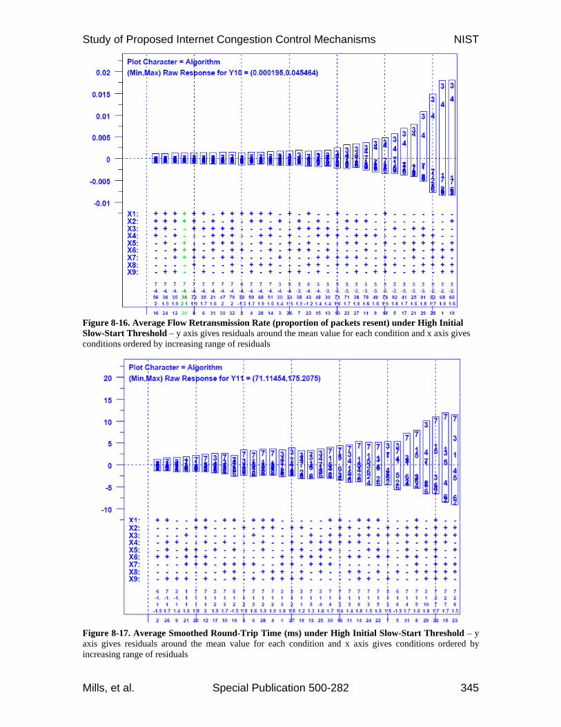
Fig. 8-16 adds more supporting evidence. Notice that FAST and FAST-AT
(algorithms 3 and 4) exhibit higher retransmission rates under conditions with higher congestion and Scalable (algorithm 7) exhibits higher retransmission rates under most other conditions. Fig. 8-17 shows that under most conditions, Scalable leads to higher average smoothed round-trip times, which supports the observation that Scalable tends to have higher buffer occupancy than other algorithms. Fig. 8-18 confirms that over an entire simulated hour, Scalable and FAST tend to complete the fewest flows. Similarly, Fig. 8-19 shows that under most conditions Scalable completes a higher proportion of flows that are small (i.e., Web objects). In the remaining conditions, either FAST or FAST-AT completes a higher proportion of flows that are Web objects. Recall that when the maximum number of flows with a given file size are already active, then newly arriving flows remain Web objects. Therefore, completing a higher proportion of flows that are Web objects implies that some larger flows (movies, service packs and documents) take longer to complete.
Study of Proposed Internet Congestion Control Mechanisms NIST
Mills, et al. Special Publication 500-282 344
Figure 8-14. Average Number of Connecting Flows under High Initial Slow-Start Threshold – y axis gives residuals around the mean value for each condition and x axis gives conditions ordered by increasing range of residuals Figure 8-15. Average Rate of Flow Completion (flows per 200 ms) under High Initial Slow-Start Threshold – y axis gives residuals around the mean value for each condition and x axis gives conditions ordered by increasing range of residuals
Study of Proposed Internet Congestion Control Mechanisms NIST
Mills, et al. Special Publication 500-282 345
Figure 8-16. Average Flow Retransmission Rate (proportion of packets resent) under High Initial Slow-Start Threshold – y axis gives residuals around the mean value for each condition and x axis gives conditions ordered by increasing range of residuals Figure 8-17. Average Smoothed Round-Trip Time (ms) under High Initial Slow-Start Threshold – y axis gives residuals around the mean value for each condition and x axis gives conditions ordered by increasing range of residuals

Study of Proposed Internet Congestion Control Mechanisms NIST
Mills, et al. Special Publication 500-282 346
Figure 8-18. Aggregate Flows Completed under High Initial Slow-Start Threshold – y axis gives residuals around the mean value for each condition and x axis gives conditions ordered by increasing range of residuals Figure 8-19. Web Objects as Proportion of Flows Completed under High Initial Slow-Start Threshold – y axis gives residuals around the mean value for each condition and x axis gives conditions ordered by increasing range of residuals
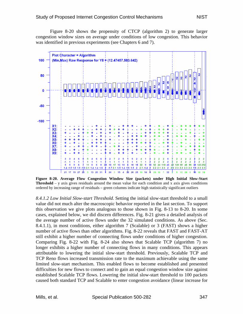
Study of Proposed Internet Congestion Control Mechanisms NIST
Mills, et al. Special Publication 500-282 347
Figure 8-20 shows the propensity of CTCP (algorithm 2) to generate larger congestion window sizes on average under conditions of low congestion. This behavior was identified in previous experiments (see Chapters 6 and 7).
Figure 8-20. Average Flow Congestion Window Size (packets) under High Initial Slow-Start Threshold – y axis gives residuals around the mean value for each condition and x axis gives conditions ordered by increasing range of residuals – green columns indicate high statistically significant outliers 8.4.1.2 Low Initial Slow-start Threshold. Setting the initial slow-start threshold to a small value did not much alter the macroscopic behavior reported in the last section. To support this observation we give plots analogous to those shown in Fig. 8-13 to 8-20. In some cases, explained below, we did discern differences. Fig. 8-21 gives a detailed analysis of the average number of active flows under the 32 simulated conditions. As above (Sec. 8.4.1.1), in most conditions, either algorithm 7 (Scalable) or 3 (FAST) shows a higher number of active flows than other algorithms. Fig. 8-22 reveals that FAST and FAST-AT still exhibit a higher number of connecting flows under conditions of higher congestion. Comparing Fig. 8-22 with Fig. 8-24 also shows that Scalable TCP (algorithm 7) no longer exhibits a higher number of connecting flows in many conditions. This appears attributable to lowering the initial slow-start threshold. Previously, Scalable TCP and TCP Reno flows increased transmission rate to the maximum achievable using the same limited slow-start mechanism. This enabled flows to become established and presented difficulties for new flows to connect and to gain an equal congestion window size against established Scalable TCP flows. Lowering the initial slow-start threshold to 100 packets caused both standard TCP and Scalable to enter congestion avoidance (linear increase for
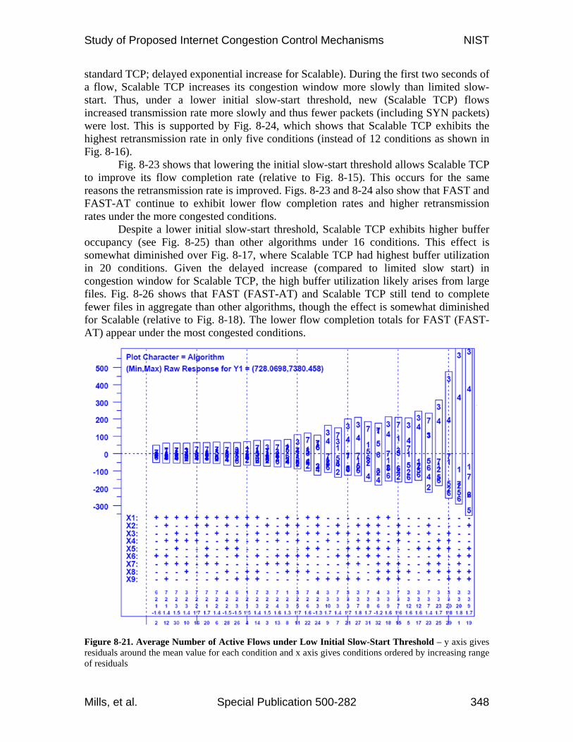
Study of Proposed Internet Congestion Control Mechanisms NIST
Mills, et al. Special Publication 500-282 348
standard TCP; delayed exponential increase for Scalable). During the first two seconds of a flow, Scalable TCP increases its congestion window more slowly than limited slow-start. Thus, under a lower initial slow-start threshold, new (Scalable TCP) flows increased transmission rate more slowly and thus fewer packets (including SYN packets) were lost. This is supported by Fig. 8-24, which shows that Scalable TCP exhibits the highest retransmission rate in only five conditions (instead of 12 conditions as shown in Fig. 8-16).
Fig. 8-23 shows that lowering the initial slow-start threshold allows Scalable TCP to improve its flow completion rate (relative to Fig. 8-15). This occurs for the same reasons the retransmission rate is improved. Figs. 8-23 and 8-24 also show that FAST and FAST-AT continue to exhibit lower flow completion rates and higher retransmission rates under the more congested conditions.
Despite a lower initial slow-start threshold, Scalable TCP exhibits higher buffer occupancy (see Fig. 8-25) than other algorithms under 16 conditions. This effect is somewhat diminished over Fig. 8-17, where Scalable TCP had highest buffer utilization in 20 conditions. Given the delayed increase (compared to limited slow start) in congestion window for Scalable TCP, the high buffer utilization likely arises from large files. Fig. 8-26 shows that FAST (FAST-AT) and Scalable TCP still tend to complete fewer files in aggregate than other algorithms, though the effect is somewhat diminished for Scalable (relative to Fig. 8-18). The lower flow completion totals for FAST (FAST-AT) appear under the most congested conditions. Figure 8-21. Average Number of Active Flows under Low Initial Slow-Start Threshold – y axis gives residuals around the mean value for each condition and x axis gives conditions ordered by increasing range of residuals
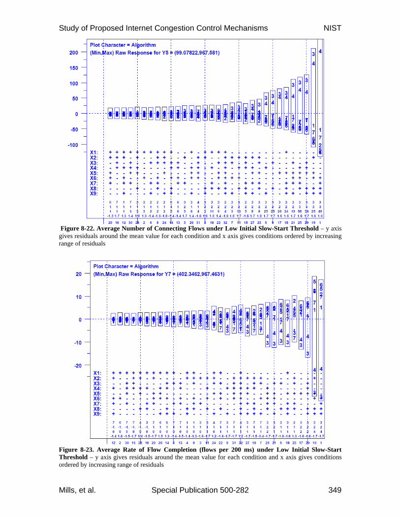
Study of Proposed Internet Congestion Control Mechanisms NIST
Mills, et al. Special Publication 500-282 349
Figure 8-22. Average Number of Connecting Flows under Low Initial Slow-Start Threshold – y axis gives residuals around the mean value for each condition and x axis gives conditions ordered by increasing range of residuals Figure 8-23. Average Rate of Flow Completion (flows per 200 ms) under Low Initial Slow-Start Threshold – y axis gives residuals around the mean value for each condition and x axis gives conditions ordered by increasing range of residuals

Study of Proposed Internet Congestion Control Mechanisms NIST
Mills, et al. Special Publication 500-282 350
Figure 8-24. Average Flow Retransmission Rate (proportion of packets resent) under Low Initial Slow-Start Threshold – y axis gives residuals around the mean value for each condition and x axis gives conditions ordered by increasing range of residuals Figure 8-25. Average Smoothed Round-Trip Time (ms) under Low Initial Slow-Start Threshold – y axis gives residuals around the mean value for each condition and x axis gives conditions ordered by increasing range of residuals

Study of Proposed Internet Congestion Control Mechanisms NIST
Mills, et al. Special Publication 500-282 351
Figure 8-26. Aggregate Flows Completed under Low Initial Slow-Start Threshold – y axis gives residuals around the mean value for each condition and x axis gives conditions ordered by increasing range of residuals
Fig. 8-27 shows that Scalable TCP completes a higher proportion of flows with small size (i.e., Web objects). This mirrors the result shown earlier in Fig. 8-19. Note, however, Fig. 8-27 reports that FAST (and FAST-AT) tend to complete a smaller proportion of flows with small size. This implies that FAST completes a higher proportion of flows with larger file size. As we demonstrate below (Sec. 8.4.2.2), this occurs because FAST increases transmission rate (after reaching the initial slow-start threshold) to the maximum available much more quickly than other algorithms.
Finally, Fig. 8-28 displays the previously demonstrated propensity of CTCP (algorithm 2) to increase congestion window to large sizes under low congestion. Given that a lower initial slow-start threshold leads to somewhat lower overall congestion (compared with a high threshold), one expects CTCP to stand out more in Fig. 8-28 than in Fig. 8-20. Comparing the two figures verifies this expectation.

Study of Proposed Internet Congestion Control Mechanisms NIST
Mills, et al. Special Publication 500-282 352
Figure 8-27. Web Objects as Proportion of Flows Completed under Low Initial Slow-Start Threshold – y axis gives residuals around the mean value for each condition and x axis gives conditions ordered by increasing range of residuals
Figure 8-28. Average Flow Congestion Window Size (packets) under Low Initial Slow-Start Threshold – y axis gives residuals around the mean value for each condition and x axis gives conditions ordered by increasing range of residuals – columns in green indicate statistically significant high outliers

Study of Proposed Internet Congestion Control Mechanisms NIST
Mills, et al. Special Publication 500-282 353
8.4.2 Absolute User Experience This section investigates absolute differences in user experience, which we measure as goodput in packets per second. We consider differences in goodput among users of the various alternate congestion control algorithms, as well as differences in goodput among TCP users competing with alternate congestion control algorithms. First, we compare these user experiences given a high initial slow-start threshold and then we compare them given a low initial slow-start threshold. Table 8-26. Average Goodput (pps) per Flow Group under Each Alternate Congestion Control Algorithm (High Initial Slow-Start Threshold)
ALTERNATE CONGESTION CONTROL ALGORITHM
File Path Interface BIC CTCP FAST FAST-AT HSTCP HTCP STCP
M
VFF 53650 50696 50299 50325 53212 49826 54638
N 7869 7846 7859 7819 7857 7834 7807
FF 8056 6451 7145 6738 7765 6295 9572
N 4789 4291 5095 4426 4694 4359 5420
TF 4843 4295 5069 4424 4698 3753 5439
N 3878 3448 4253 3527 3749 3162 4446
SP
VFF 24911 25410 25555 25727 24675 25274 24694
N 7262 7313 7340 7346 7242 7295 7168
FF 6655 6073 6563 6722 6472 5830 6935
N 4679 4456 4934 5002 4563 4328 4801
TF 4870 4421 5075 5142 4617 4094 5164
N 4053 3789 4364 4398 3876 3513 4225
D
VFF 2008 2099 2088 2078 2025 2084 1989
N 1800 1833 1833 1830 1787 1834 1782
FF 1189 1213 1175 1203 1201 1220 1174
N 1124 1149 1113 1140 1138 1162 1111
TF 1308 1315 1291 1310 1313 1330 1293
N 1254 1264 1240 1259 1261 1281 1240
WO
VFF 366 390 378 360 427 428 378
N 384 395 395 394 382 394 379
FF 255 261 250 256 258 263 252
N 250 256 245 251 253 258 247
TF 308 313 301 306 312 318 306
N 303 307 296 300 307 312 300
8.4.2.1 High Initial Slow-start Threshold. Table 8-26 summarizes the average goodput – response y2(u) – experienced by users in each of the 24 flow classes (dimensioned by file size, path quality and interface speed) under each of the seven alternate congestion control algorithms. Table 8-27 provides a similar summary of the average goodput – response y16(u) – experienced by TCP users in each of the 24 flow classes when competing with flows in each of the seven alternate congestion control algorithms. Since the tables are somewhat dense with numbers, we present this information in the form of bar graphs (Fig. 8-29 through 8-32) – one figure per file size: movie, service pack, document and Web object. (The legend for the bar graphs is shown in Fig. 8-7.) The top
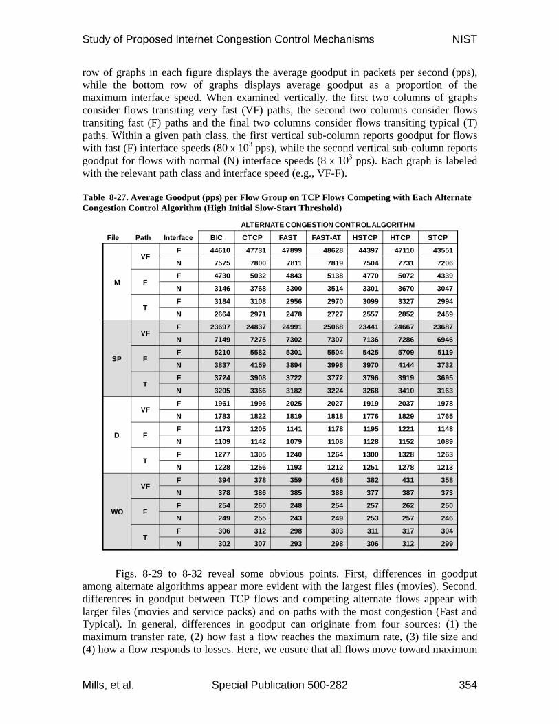
Study of Proposed Internet Congestion Control Mechanisms NIST
Mills, et al. Special Publication 500-282 354
row of graphs in each figure displays the average goodput in packets per second (pps), while the bottom row of graphs displays average goodput as a proportion of the maximum interface speed. When examined vertically, the first two columns of graphs consider flows transiting very fast (VF) paths, the second two columns consider flows transiting fast (F) paths and the final two columns consider flows transiting typical (T) paths. Within a given path class, the first vertical sub-column reports goodput for flows with fast (F) interface speeds (80 x 103 pps), while the second vertical sub-column reports goodput for flows with normal (N) interface speeds (8 x 10³ pps). Each graph is labeled with the relevant path class and interface speed (e.g., VF-F). Table 8-27. Average Goodput (pps) per Flow Group on TCP Flows Competing with Each Alternate Congestion Control Algorithm (High Initial Slow-Start Threshold)
ALTERNATE CONGESTION CONTROL ALGORITHM
File Path Interface BIC CTCP FAST FAST-AT HSTCP HTCP STCP
M
VFF 44610 47731 47899 48628 44397 47110 43551
N 7575 7800 7811 7819 7504 7731 7206
FF 4730 5032 4843 5138 4770 5072 4339
N 3146 3768 3300 3514 3301 3670 3047
TF 3184 3108 2956 2970 3099 3327 2994
N 2664 2971 2478 2727 2557 2852 2459
SP
VFF 23697 24837 24991 25068 23441 24667 23687
N 7149 7275 7302 7307 7136 7286 6946
FF 5210 5582 5301 5504 5425 5709 5119
N 3837 4159 3894 3998 3970 4144 3732
TF 3724 3908 3722 3772 3796 3919 3695
N 3205 3366 3182 3224 3268 3410 3163
D
VFF 1961 1996 2025 2027 1919 2037 1978
N 1783 1822 1819 1818 1776 1829 1765
FF 1173 1205 1141 1178 1195 1221 1148
N 1109 1142 1079 1108 1128 1152 1089
TF 1277 1305 1240 1264 1300 1328 1263
N 1228 1256 1193 1212 1251 1278 1213
WO
VFF 394 378 359 458 382 431 358
N 378 386 385 388 377 387 373
FF 254 260 248 254 257 262 250
N 249 255 243 249 253 257 246
TF 306 312 298 303 311 317 304
N 302 307 293 298 306 312 299
Figs. 8-29 to 8-32 reveal some obvious points. First, differences in goodput
among alternate algorithms appear more evident with the largest files (movies). Second, differences in goodput between TCP flows and competing alternate flows appear with larger files (movies and service packs) and on paths with the most congestion (Fast and Typical). In general, differences in goodput can originate from four sources: (1) the maximum transfer rate, (2) how fast a flow reaches the maximum rate, (3) file size and (4) how a flow responds to losses. Here, we ensure that all flows move toward maximum

Study of Proposed Internet Congestion Control Mechanisms NIST
Mills, et al. Special Publication 500-282 355
transfer rate at the same speed (by using limited slow-start until the first packet loss). We devote each figure to only one file size. This means that any goodput differences in each figure (for Figs. 8-28 to 8-32) can result only from loss processing. In other words, how much does a flow slow its transmission rate after a loss and how quickly does it recover? We expect all alternate congestion control algorithms to improve over TCP Reno with respect to processing losses, so we expect differences to appear on congested paths and on larger flows which exhibit a larger probability of loss/recovery events. Flows transmitting small files should not experience as many loss/recovery cycles as flows transmitting large files. Similarly, flows crossing uncongested paths should not experience as many loss/recovery cycles as flows transiting congested paths. Figure 8-29. Average Goodput on Movies (High Initial Slow-Start Threshold) (Top row shows raw goodput in pps and bottom row shows goodput as a proportion of interface speed)
Though Figs. 8-29 to 8-32 reveal some modest differences in goodput among
flows groups based on congestion control algorithm, we suspected that more significant goodput variations in the data would be explained by differences in experiment conditions. To investigate, we conducted a principal components analysis (PCA) of the average goodput data across all flow groups. Fig. 8-33 plots the resulting information, which reveals three main groups: (1) a group where network speed is low (factor x1 = -1), (2) a group where network speed is high (factor x1 = +1) and propagation delay is high (factor x2 = +1) and (3) a group where network speed is high and propagation delay is low (factor x2 = -1). Each of the latter two groups could be divided into two subgroups based on average file size: (a) smaller (x5 = -1) and (b) larger (x5 = +1). No distinct collection of congestion control algorithms appears anywhere in Fig. 8-33. This suggests that most of the variation in the data under a high initial slow-start threshold arises from network speed, propagation delay and file size. The congestion control algorithm has
VF-F VF-N F-F F-N T-F T-N
VF-F VF-N F-F F-N T-F T-N
VF-F VF-N F-F F-N T-F T-NVF-F VF-N F-F F-N T-F T-N
VF-F VF-N F-F F-N T-F T-NVF-F VF-N F-F F-N T-F T-NVF-F VF-N F-F F-N T-F T-N
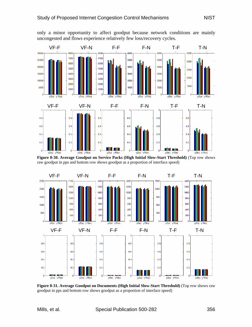
Study of Proposed Internet Congestion Control Mechanisms NIST
Mills, et al. Special Publication 500-282 356
only a minor opportunity to affect goodput because network conditions are mainly uncongested and flows experience relatively few loss/recovery cycles. Figure 8-30. Average Goodput on Service Packs (High Initial Slow-Start Threshold) (Top row shows raw goodput in pps and bottom row shows goodput as a proportion of interface speed) Figure 8-31. Average Goodput on Documents (High Initial Slow-Start Threshold) (Top row shows raw goodput in pps and bottom row shows goodput as a proportion of interface speed)
VF-F VF-N F-F F-N T-F T-N
VF-F VF-N F-F F-N T-F T-N
VF-F VF-N F-F F-N T-F T-NVF-F VF-N F-F F-N T-F T-NVF-F VF-N F-F F-N T-F T-N
VF-F VF-N F-F F-N T-F T-NVF-F VF-N F-F F-N T-F T-NVF-F VF-N F-F F-N T-F T-N
VF-F VF-N F-F F-N T-F T-N
VF-F VF-N F-F F-N T-F T-N
VF-F VF-N F-F F-N T-F T-NVF-F VF-N F-F F-N T-F T-NVF-F VF-N F-F F-N T-F T-N
VF-F VF-N F-F F-N T-F T-NVF-F VF-N F-F F-N T-F T-NVF-F VF-N F-F F-N T-F T-N
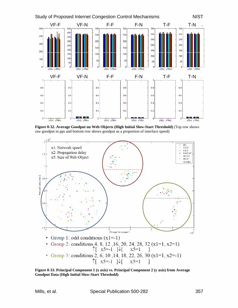
Study of Proposed Internet Congestion Control Mechanisms NIST
Mills, et al. Special Publication 500-282 357
Figure 8-32. Average Goodput on Web Objects (High Initial Slow-Start Threshold) (Top row shows raw goodput in pps and bottom row shows goodput as a proportion of interface speed) Figure 8-33. Principal Component 1 (x axis) vs. Principal Component 2 (y axis) from Average Goodput Data (High Initial Slow-Start Threshold)
VF-F VF-N F-F F-N T-F T-N
VF-F VF-N F-F F-N T-F T-N
VF-F VF-N F-F F-N T-F T-NVF-F VF-N F-F F-N T-F T-N
VF-F VF-N F-F F-N T-F T-NVF-F VF-N F-F F-N T-F T-N
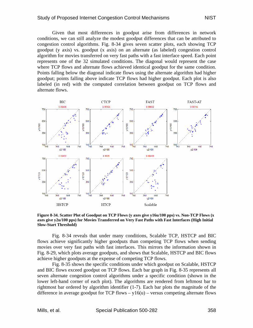
Study of Proposed Internet Congestion Control Mechanisms NIST
Mills, et al. Special Publication 500-282 358
Given that most differences in goodput arise from differences in network conditions, we can still analyze the modest goodput differences that can be attributed to congestion control algorithms. Fig. 8-34 gives seven scatter plots, each showing TCP goodput (y axis) vs. goodput (x axis) on an alternate (as labeled) congestion control algorithm for movies transferred on very fast paths with a fast interface speed. Each point represents one of the 32 simulated conditions. The diagonal would represent the case where TCP flows and alternate flows achieved identical goodput for the same condition. Points falling below the diagonal indicate flows using the alternate algorithm had higher goodput; points falling above indicate TCP flows had higher goodput. Each plot is also labeled (in red) with the computed correlation between goodput on TCP flows and alternate flows. Figure 8-34. Scatter Plot of Goodput on TCP Flows (y axes give y16u/100 pps) vs. Non-TCP Flows (x axes give y2u/100 pps) for Movies Transferred on Very Fast Paths with Fast Interfaces (High Initial Slow-Start Threshold)
Fig. 8-34 reveals that under many conditions, Scalable TCP, HSTCP and BIC flows achieve significantly higher goodputs than competing TCP flows when sending movies over very fast paths with fast interfaces. This mirrors the information shown in Fig. 8-29, which plots average goodputs, and shows that Scalable, HSTCP and BIC flows achieve higher goodputs at the expense of competing TCP flows.
Fig. 8-35 shows the specific conditions under which goodput on Scalable, HSTCP and BIC flows exceed goodput on TCP flows. Each bar graph in Fig. 8-35 represents all seven alternate congestion control algorithms under a specific condition (shown in the lower left-hand corner of each plot). The algorithms are rendered from leftmost bar to rightmost bar ordered by algorithm identifier (1-7). Each bar plots the magnitude of the difference in average goodput for TCP flows – y16(u) – versus competing alternate flows

Study of Proposed Internet Congestion Control Mechanisms NIST
Mills, et al. Special Publication 500-282 359
– y2(u). If the bar is red, y16(u) is greater; if the bar is green, y2(u) is greater. The 32 bar graphs are sorted from least to most congestion. Figure 8-35. 32 Bar Graphs (one for each Simulated Condition) plotting Goodput (pps/1000) on TCP Flows vs. Non-TCP Flows for Movies Transferred on Very Fast Paths with Fast Interfaces (High Initial Slow-Start Threshold) (Each graph contains seven bars, one per congestion control algorithm, ordered left to right by algorithm identifier. Each bar plots the magnitude of the difference in average goodput for TCP flows – y16(u) – versus competing alternate flows – y2(u). If the bar is red, y16(u) is greater; if the bar is green, y2(u) is greater. The 32 bar graphs are sorted from least to most congestion by condition, as indicated in the lower left-hand corner of each plot.)
Fig. 8-35 reveals scant differences in goodput between TCP flows and alternate flows under the 16 least congested conditions. Differences in goodput between alternate flows and TCP flows increase with increasing congestion for BIC, HSTCP and Scalable. This reveals that aspects of loss/recovery processing implemented by BIC, HSTCP and Scalable penalize TCP flows. As discussed previously, in Chapter 6, Scalable TCP (along with BIC and HSTCP) reduce congestion window size much less than TCP flows in response to a single loss, so once a Scalable flow establishes a large congestion window and related buffer space along a path, it could take many loss events to significantly reduce the flow’s transmission rate. TCP flows, on the other hand, reduce the congestion window by half on each loss and thus TCP flows reduce transmission rate much faster than Scalable TCP flows.

Study of Proposed Internet Congestion Control Mechanisms NIST
Mills, et al. Special Publication 500-282 360
Figure 8-36. Scatter Plot of Goodput on TCP Flows (y axes give y16u/100 pps) vs. Non-TCP Flows (x axes give y2u/100 pps) for Service Packs Transferred on Very Fast Paths with Fast Interfaces (High Initial Slow-Start Threshold) Figure 8-37. Scatter Plot of Goodput on TCP Flows (y axes give y16u/100 pps) vs. Non-TCP Flows (x axes give y2u/100 pps) for Documents Transferred on Very Fast Paths with Fast Interfaces (High Initial Slow-Start Threshold)
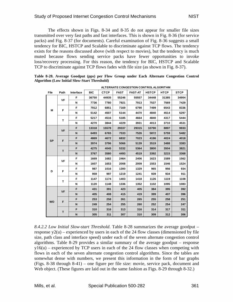
Study of Proposed Internet Congestion Control Mechanisms NIST
Mills, et al. Special Publication 500-282 361
The effects shown in Figs. 8-34 and 8-35 do not appear for smaller file sizes transmitted over very fast paths and fast interfaces. This is shown in Fig. 8-36 (for service packs) and Fig. 8-37 (for documents). Careful examination of Fig. 8-36 suggests a small tendency for BIC, HSTCP and Scalable to discriminate against TCP flows. The tendency exists for the reasons discussed above (with respect to movies), but the tendency is much muted because flows sending service packs have fewer opportunities to invoke loss/recovery processing. For this reason, the tendency for BIC, HSTCP and Scalable TCP to discriminate against TCP flows fades with file size (as shown in Fig. 8-37).
Table 8-28. Average Goodput (pps) per Flow Group under Each Alternate Congestion Control Algorithm (Low Initial Slow-Start Threshold)
ALTERNATE CONGESTION CONTROL ALGORITHM
File Path Interface BIC CTCP FAST FAST-AT HSTCP HTCP STCP
M
VFF 36750 44935 55246 55557 34448 31385 34904
N 7736 7780 7921 7913 7537 7569 7429
FF 7912 6851 7169 6790 7499 6543 8336
N 5142 4507 5144 4470 4840 4514 5297
TF 5217 4516 5185 4664 4840 4317 5444
N 4270 3844 4229 3931 4013 3710 4531
SP
VFF 13318 15578 29337 29315 10790 8897 9933
N 6493 6765 7533 7526 5872 5759 5482
FF 4869 4672 6832 7023 4196 4024 4018
N 3974 3796 5066 5139 3519 3488 3383
TF 4275 4045 5332 5364 3800 3504 3821
N 3767 3580 4493 4519 3392 3215 3368
D
VFF 1669 1682 2464 2406 1623 1589 1562
N 1607 1653 2008 2009 1553 1546 1524
FF 987 1016 1300 1329 965 956 934
N 959 997 1219 1241 939 934 911
TF 1147 1174 1403 1418 1126 1119 1108
N 1120 1148 1336 1352 1102 1095 1083
WO
VFF 431 391 423 405 384 395 392
N 405 408 415 419 399 407 396
FF 253 258 261 265 255 258 251
N 249 254 255 260 252 254 247
TF 310 316 313 316 314 317 311
N 305 311 307 310 309 312 306
8.4.2.2 Low Initial Slow-start Threshold. Table 8-28 summarizes the average goodput – response y2(u) – experienced by users in each of the 24 flow classes (dimensioned by file size, path class and interface speed) under each of the seven alternate congestion control algorithms. Table 8-29 provides a similar summary of the average goodput – response y16(u) – experienced by TCP users in each of the 24 flow classes when competing with flows in each of the seven alternate congestion control algorithms. Since the tables are somewhat dense with numbers, we present this information in the form of bar graphs (Figs. 8-38 through 8-41) – one figure per file size: movie, service pack, document and Web object. (These figures are laid out in the same fashion as Figs. 8-29 through 8-32.)

Study of Proposed Internet Congestion Control Mechanisms NIST
Mills, et al. Special Publication 500-282 362
Tables 8-28 and 8-29, as well as Figs. 8-38 to 8-40, show a marked increase in
goodput differences among flows using alternate congestion control algorithms and between flows using alternate congestion control algorithms and flows using TCP. These increased differences must arise from reducing the initial slow-start threshold to a low value, as all other aspects of the simulations remained the same. Table 8-29. Average Goodput (pps) per Flow Group on TCP Flows Competing with Each Alternate Congestion Control Algorithm (Low Initial Slow-Start Threshold)
ALTERNATE CONGESTION CONTROL ALGORITHM
File Path Interface BIC CTCP FAST FAST-AT HSTCP HTCP STCP
M
VFF 16053 16621 16951 16774 16279 16833 16228
N 7014 7068 7065 7080 6968 6958 6857
FF 4532 4821 4246 4330 4651 4859 4253
N 3286 3756 3383 3282 3542 3468 3406
TF 3380 3822 3098 3158 3662 3580 3451
N 2963 3298 2780 2832 3125 3240 3028
SP
VFF 6484 6531 6563 6494 6498 6636 6456
N 4838 4939 4950 4959 4847 4888 4771
FF 2872 2936 2709 2762 2886 3037 2818
N 2569 2717 2520 2523 2642 2704 2589
TF 2811 2916 2562 2627 2872 2941 2861
N 2592 2738 2391 2444 2668 2730 2652
D
VFF 1504 1528 1521 1521 1493 1561 1520
N 1509 1516 1518 1514 1504 1524 1500
FF 919 941 899 913 939 950 920
N 897 920 873 892 914 929 897
TF 1076 1098 1031 1043 1098 1113 1084
N 1054 1076 1009 1023 1077 1091 1063
WO
VFF 379 404 389 396 396 392 385
N 396 397 397 397 388 396 388
FF 250 255 246 250 254 258 250
N 246 251 242 246 250 253 246
TF 307 312 298 301 312 316 310
N 303 308 294 297 308 312 305
Figs. 8-38 to 8-41 reveal some obvious points. First, flows using alternate
congestion control algorithms often achieve much higher goodputs than flows using TCP congestion control. The differences increase with file size and with interface speed. For the smallest size (Web objects, Fig. 8-41) there is no appreciable goodput difference among flows. Second, FAST and FAST-AT flows achieve markedly higher goodputs than flows using the other alternate congestion control protocols. The ability of FAST flows to achieve higher goodputs must arise from differences in congestion window increase procedures after a flow reaches the initial slow-start threshold. Third, the tendency of Scalable TCP, BIC and HSTCP flows to discriminate against TCP flows
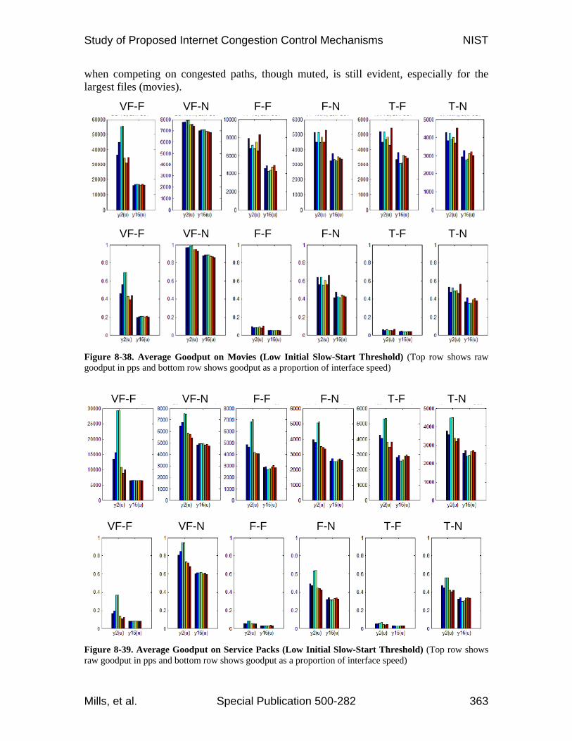
Study of Proposed Internet Congestion Control Mechanisms NIST
Mills, et al. Special Publication 500-282 363
when competing on congested paths, though muted, is still evident, especially for the largest files (movies).
Figure 8-38. Average Goodput on Movies (Low Initial Slow-Start Threshold) (Top row shows raw goodput in pps and bottom row shows goodput as a proportion of interface speed) Figure 8-39. Average Goodput on Service Packs (Low Initial Slow-Start Threshold) (Top row shows raw goodput in pps and bottom row shows goodput as a proportion of interface speed)
VF-F VF-N F-F F-N T-F T-N
VF-F VF-N F-F F-N T-F T-N
VF-F VF-N F-F F-N T-F T-NVF-F VF-N F-F F-N T-F T-N
VF-F VF-N F-F F-N T-F T-NVF-F VF-N F-F F-N T-F T-N
VF-F VF-N F-F F-N T-F T-N
VF-F VF-N F-F F-N T-F T-N
VF-F VF-N F-F F-N T-F T-NVF-F VF-N F-F F-N T-F T-N
VF-F VF-N F-F F-N T-F T-NVF-F VF-N F-F F-N T-F T-N
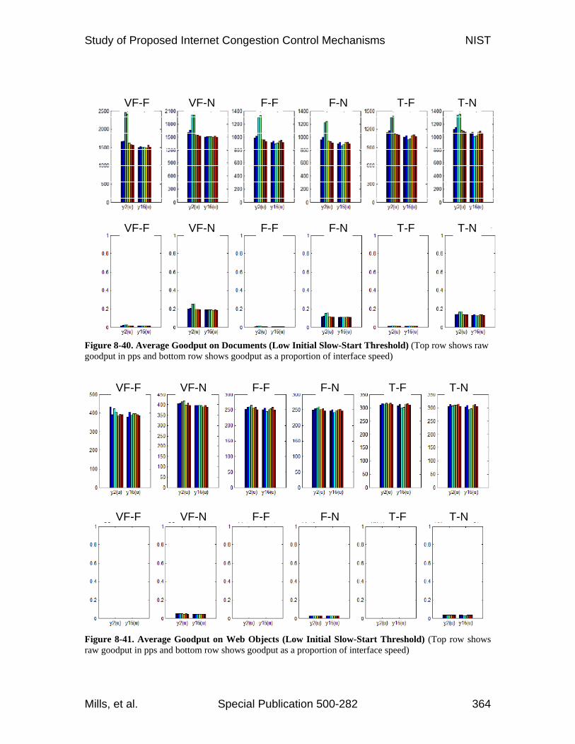
Study of Proposed Internet Congestion Control Mechanisms NIST
Mills, et al. Special Publication 500-282 364
Figure 8-40. Average Goodput on Documents (Low Initial Slow-Start Threshold) (Top row shows raw goodput in pps and bottom row shows goodput as a proportion of interface speed) Figure 8-41. Average Goodput on Web Objects (Low Initial Slow-Start Threshold) (Top row shows raw goodput in pps and bottom row shows goodput as a proportion of interface speed)
VF-F VF-N F-F F-N T-F T-N
VF-F VF-N F-F F-N T-F T-N
VF-F VF-N F-F F-N T-F T-NVF-F VF-N F-F F-N T-F T-N
VF-F VF-N F-F F-N T-F T-NVF-F VF-N F-F F-N T-F T-N
VF-F VF-N F-F F-N T-F T-N
VF-F VF-N F-F F-N T-F T-N
VF-F VF-N F-F F-N T-F T-NVF-F VF-N F-F F-N T-F T-N
VF-F VF-N F-F F-N T-F T-NVF-F VF-N F-F F-N T-F T-N

Study of Proposed Internet Congestion Control Mechanisms NIST
Mills, et al. Special Publication 500-282 365
Though Figs. 8-38 to 8-40 reveal strong differences in goodput for flow groups using FAST and FAST-AT, we wanted to investigate to what extent differences in experiment conditions drove differences in goodput. To investigate this question, we conducted a principal components analysis (PCA) of the average goodput data across all flow groups. Fig. 8-42 plots the resulting information (a biplot of the first two principal components), which reveals two main groups of points: (1) goodput when network speed was lower (x1 = -1) and (2) goodput when network speed was higher (x1 = +1). This is as expected: higher network speeds enable higher goodputs. Fig. 8-42 also reveals differences with respect to congestion control algorithm. Note that goodputs for flows using algorithm 3 (FAST) and algorithm 4 (FAST-AT) tend toward the right-hand side of the plot and there is a rightmost grouping of points associated with FAST and FAST-AT.5 These points represent cases when network speed is high and propagation delay is low (x2 = -1). This suggests that FAST and FAST-AT can achieve significantly higher goodputs than other congestion control algorithms under such conditions. Figure 8-42. Principal Component 1 (x axis) vs. Principal Component 2 (y axis) for Average Goodput Data (Low Initial Slow-Start Threshold)
5 Though the data included goodput for TCP flows, differences in goodput among TCP flows was far overshadowed by differences in goodput for algorithm 3 (FAST) and algorithm 4 (FAST-AT) flows compared to flows using other alternate congestion control algorithms.

Study of Proposed Internet Congestion Control Mechanisms NIST
Mills, et al. Special Publication 500-282 366
Fig. 8-43 gives seven scatter plots, each showing TCP goodput (y axis) vs. goodput on an alternate (as labeled) congestion control algorithm for movies transferred on very fast paths with a fast interface speed. Comparing Fig. 8-43 with Fig. 8-34, which gives the same information under high initial slow-start threshold, shows marked differences. Under low initial slow-start threshold, all seven alternate congestion control protocols provide much better goodput than achieved on TCP flows. This result can be attributed directly to the adoption of a low initial slow-start threshold. After reaching a congestion window size of 100 packets, the increase functions of the congestion avoidance regime of each protocol are activated. The TCP congestion avoidance regime leads to linear increase in transmission rate, while the congestion avoidance regimes in the other protocols lead to greater than linear increase. The precise increase rate depends upon the specific algorithm. Fig. 8-44 shows the degree to which goodput on flows using each alternate congestion control algorithm exceeds goodput on TCP flows for each condition when movies are transferred on very fast paths with a fast interface speed. Figure 8-43. Scatter Plot of Goodput on TCP Flows (y axes give y16u/100 pps) vs. Non-TCP Flows (x axes give y2u/100 pps) for Movies Transferred on Very Fast Paths with Fast Interfaces (Low Initial Slow-Start Threshold)
Fig. 8-44 confirms the results in Fig. 8-43 and also reveals that flows using FAST and FAST-AT achieve higher goodput advantage over TCP flows, though the advantage diminishes somewhat with increasing congestion. This means that, in congestion avoidance, FAST increases transmission rate faster than the other congestion control algorithms. From Fig. 8-44 one can also discern that CTCP increases transmission rate second fastest. Thus, when given a low initial slow-start threshold and transferring large files at high speeds over paths with little congestion, the congestion avoidance increase procedures of the alternate protocols reach maximum transfer rate far more quickly than possible using the linear increase procedures of TCP. This general pattern also holds for

Study of Proposed Internet Congestion Control Mechanisms NIST
Mills, et al. Special Publication 500-282 367
service packs (see Figs. 8-45 and 8-46) and documents (see Figs. 8-47 and 8-48). Note that for these smaller file sizes FAST and FAST-AT still achieve much higher goodputs than normal TCP, though the degree to which the other alternate congestion control algorithms outperform TCP is much diminished.
Figure 8-44. 32 Bar Graphs (one for each simulated condition) plotting Goodput (pps/1000) on TCP Flows vs. Non-TCP Flows for Movies Transferred on Very Fast Paths with Fast Interfaces (Low Initial Slow-Start Threshold) (Each graph contains seven bars, one per congestion control algorithm, ordered left to right by algorithm identifier. Each bar plots the magnitude of the difference in average goodput for TCP flows – y16(u) – versus competing alternate flows – y2(u).)
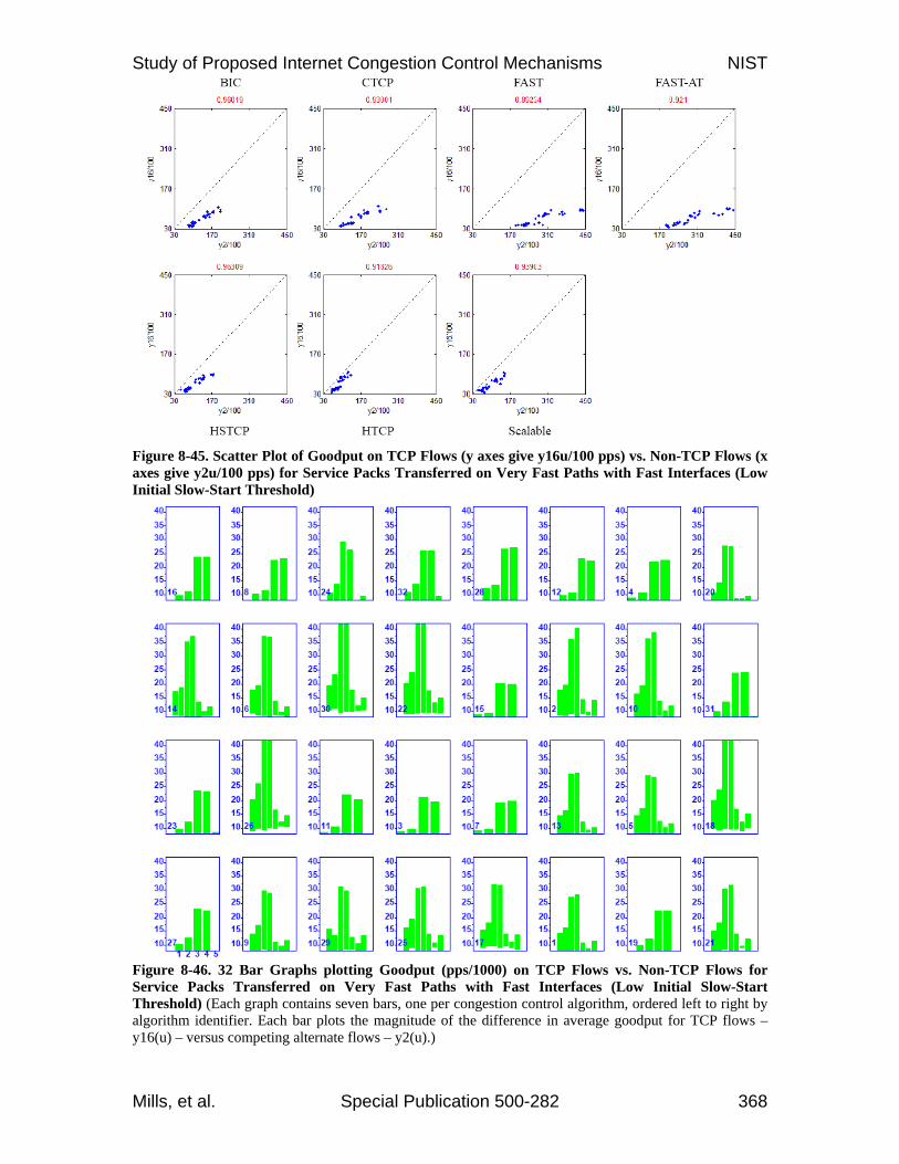
Study of Proposed Internet Congestion Control Mechanisms NIST
Mills, et al. Special Publication 500-282 368
Figure 8-45. Scatter Plot of Goodput on TCP Flows (y axes give y16u/100 pps) vs. Non-TCP Flows (x axes give y2u/100 pps) for Service Packs Transferred on Very Fast Paths with Fast Interfaces (Low Initial Slow-Start Threshold) Figure 8-46. 32 Bar Graphs plotting Goodput (pps/1000) on TCP Flows vs. Non-TCP Flows for Service Packs Transferred on Very Fast Paths with Fast Interfaces (Low Initial Slow-Start Threshold) (Each graph contains seven bars, one per congestion control algorithm, ordered left to right by algorithm identifier. Each bar plots the magnitude of the difference in average goodput for TCP flows – y16(u) – versus competing alternate flows – y2(u).)

Study of Proposed Internet Congestion Control Mechanisms NIST
Mills, et al. Special Publication 500-282 369
Figure 8-47. Scatter Plot of Goodput on TCP Flows (y axes give y16u/100 pps) vs. Non-TCP Flows (x axes give y2u/100 pps) for Documents Transferred on Very Fast Paths with Fast Interfaces (Low Initial Slow-Start Threshold) Figure 8-48. 32 Bar Graphs plotting Goodput (pps/1000) on TCP Flows vs. Non-TCP Flows for Service Packs Transferred on Very Fast Paths with Fast Interfaces (Low Initial Slow-Start Threshold) (Each graph contains seven bars, one per congestion control algorithm, ordered left to right by algorithm identifier. Each bar plots the magnitude of the difference in average goodput for TCP flows – y16(u) – versus competing alternate flows – y2(u). If the bar is red, y16(u) is greater; if the bar is green, y2(u) is greater. The 32 bar graphs are sorted from least to most congestion by condition, as indicated in the lower left-hand corner of each plot.)
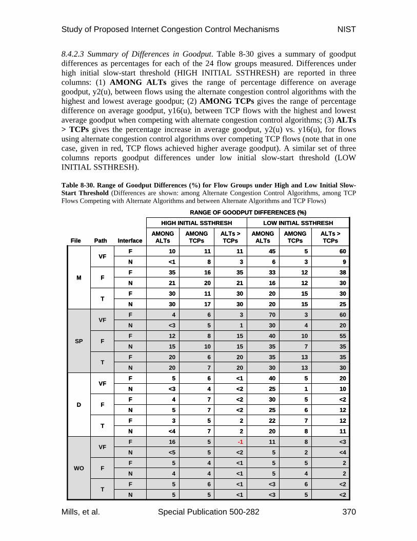
Study of Proposed Internet Congestion Control Mechanisms NIST
Mills, et al. Special Publication 500-282 370
8.4.2.3 Summary of Differences in Goodput. Table 8-30 gives a summary of goodput differences as percentages for each of the 24 flow groups measured. Differences under high initial slow-start threshold (HIGH INITIAL SSTHRESH) are reported in three columns: (1) AMONG ALTs gives the range of percentage difference on average goodput, y2(u), between flows using the alternate congestion control algorithms with the highest and lowest average goodput; (2) AMONG TCPs gives the range of percentage difference on average goodput, y16(u), between TCP flows with the highest and lowest average goodput when competing with alternate congestion control algorithms; (3) ALTs > TCPs gives the percentage increase in average goodput, y2(u) vs. y16(u), for flows using alternate congestion control algorithms over competing TCP flows (note that in one case, given in red, TCP flows achieved higher average goodput). A similar set of three columns reports goodput differences under low initial slow-start threshold (LOW INITIAL SSTHRESH). Table 8-30. Range of Goodput Differences (%) for Flow Groups under High and Low Initial Slow-Start Threshold (Differences are shown: among Alternate Congestion Control Algorithms, among TCP Flows Competing with Alternate Algorithms and between Alternate Algorithms and TCP Flows)
LOW INITIAL SSTHRESHHIGH INITIAL SSTHRESH
<26<3<165FT
<25<3<155N
245<144N
255<145FF
<425<25<5N
<3811-1516FVF
WO
1182027<4N
12722253FT
12625<275N
<2530<274FF
10125<24<3N
20540<165FVF
D
30133020720N
35133520620FT
35735151015N
55104015812FF
2043015<3N
60370364FVF
SP
251520301730N
301520301130FT
301216212021N
381233351635FF
93638<1N
60545111110FVF
M
ALTs > TCPs
AMONG TCPs
AMONG ALTs
ALTs > TCPs
AMONG TCPs
AMONG ALTsInterfacePathFile
RANGE OF GOODPUT DIFFERENCES (%)
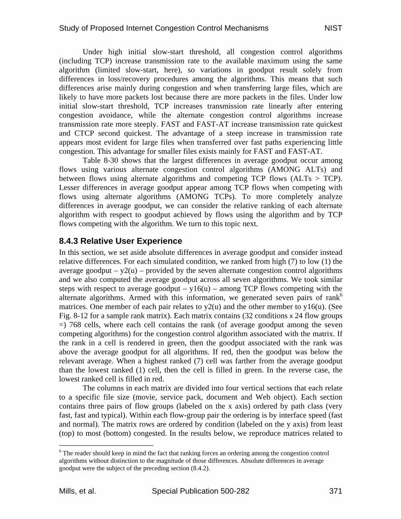
Study of Proposed Internet Congestion Control Mechanisms NIST
Mills, et al. Special Publication 500-282 371
Under high initial slow-start threshold, all congestion control algorithms (including TCP) increase transmission rate to the available maximum using the same algorithm (limited slow-start, here), so variations in goodput result solely from differences in loss/recovery procedures among the algorithms. This means that such differences arise mainly during congestion and when transferring large files, which are likely to have more packets lost because there are more packets in the files. Under low initial slow-start threshold, TCP increases transmission rate linearly after entering congestion avoidance, while the alternate congestion control algorithms increase transmission rate more steeply. FAST and FAST-AT increase transmission rate quickest and CTCP second quickest. The advantage of a steep increase in transmission rate appears most evident for large files when transferred over fast paths experiencing little congestion. This advantage for smaller files exists mainly for FAST and FAST-AT.
Table 8-30 shows that the largest differences in average goodput occur among flows using various alternate congestion control algorithms (AMONG ALTs) and between flows using alternate algorithms and competing TCP flows (ALTs > TCP). Lesser differences in average goodput appear among TCP flows when competing with flows using alternate algorithms (AMONG TCPs). To more completely analyze differences in average goodput, we can consider the relative ranking of each alternate algorithm with respect to goodput achieved by flows using the algorithm and by TCP flows competing with the algorithm. We turn to this topic next.
8.4.3 Relative User Experience In this section, we set aside absolute differences in average goodput and consider instead relative differences. For each simulated condition, we ranked from high (7) to low (1) the average goodput – y2(u) – provided by the seven alternate congestion control algorithms and we also computed the average goodput across all seven algorithms. We took similar steps with respect to average goodput – y16(u) – among TCP flows competing with the alternate algorithms. Armed with this information, we generated seven pairs of rank6 matrices. One member of each pair relates to y2(u) and the other member to y16(u). (See Fig. 8-12 for a sample rank matrix). Each matrix contains (32 conditions x 24 flow groups =) 768 cells, where each cell contains the rank (of average goodput among the seven competing algorithms) for the congestion control algorithm associated with the matrix. If the rank in a cell is rendered in green, then the goodput associated with the rank was above the average goodput for all algorithms. If red, then the goodput was below the relevant average. When a highest ranked (7) cell was farther from the average goodput than the lowest ranked (1) cell, then the cell is filled in green. In the reverse case, the lowest ranked cell is filled in red.
The columns in each matrix are divided into four vertical sections that each relate to a specific file size (movie, service pack, document and Web object). Each section contains three pairs of flow groups (labeled on the x axis) ordered by path class (very fast, fast and typical). Within each flow-group pair the ordering is by interface speed (fast and normal). The matrix rows are ordered by condition (labeled on the y axis) from least (top) to most (bottom) congested. In the results below, we reproduce matrices related to 6 The reader should keep in mind the fact that ranking forces an ordering among the congestion control algorithms without distinction to the magnitude of those differences. Absolute differences in average goodput were the subject of the preceding section (8.4.2).
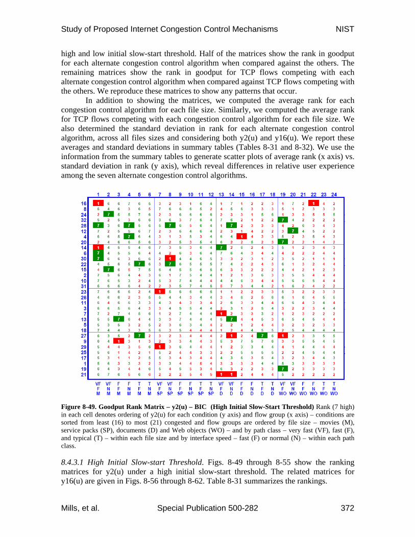
Study of Proposed Internet Congestion Control Mechanisms NIST
Mills, et al. Special Publication 500-282 372
high and low initial slow-start threshold. Half of the matrices show the rank in goodput for each alternate congestion control algorithm when compared against the others. The remaining matrices show the rank in goodput for TCP flows competing with each alternate congestion control algorithm when compared against TCP flows competing with the others. We reproduce these matrices to show any patterns that occur.
In addition to showing the matrices, we computed the average rank for each congestion control algorithm for each file size. Similarly, we computed the average rank for TCP flows competing with each congestion control algorithm for each file size. We also determined the standard deviation in rank for each alternate congestion control algorithm, across all files sizes and considering both y2(u) and y16(u). We report these averages and standard deviations in summary tables (Tables 8-31 and 8-32). We use the information from the summary tables to generate scatter plots of average rank (x axis) vs. standard deviation in rank (y axis), which reveal differences in relative user experience among the seven alternate congestion control algorithms.
Figure 8-49. Goodput Rank Matrix – y2(u) – BIC (High Initial Slow-Start Threshold) Rank (7 high) in each cell denotes ordering of y2(u) for each condition (y axis) and flow group (x axis) – conditions are sorted from least (16) to most (21) congested and flow groups are ordered by file size – movies (M), service packs (SP), documents (D) and Web objects (WO) – and by path class – very fast (VF), fast (F), and typical (T) – within each file size and by interface speed – fast (F) or normal (N) – within each path class.
8.4.3.1 High Initial Slow-start Threshold. Figs. 8-49 through 8-55 show the ranking matrices for y2(u) under a high initial slow-start threshold. The related matrices for y16(u) are given in Figs. 8-56 through 8-62. Table 8-31 summarizes the rankings.
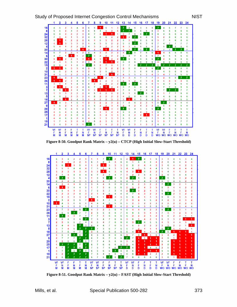
Study of Proposed Internet Congestion Control Mechanisms NIST
Mills, et al. Special Publication 500-282 373
Figure 8-50. Goodput Rank Matrix – y2(u) – CTCP (High Initial Slow-Start Threshold)
Figure 8-51. Goodput Rank Matrix – y2(u) – FAST (High Initial Slow-Start Threshold)

Study of Proposed Internet Congestion Control Mechanisms NIST
Mills, et al. Special Publication 500-282 374
Figure 8-52. Goodput Rank Matrix – y2(u) – FAST-AT (High Initial Slow-Start Threshold)
Figure 8-53. Goodput Rank Matrix – y2(u) – HSTCP (High Initial Slow-Start Threshold)

Study of Proposed Internet Congestion Control Mechanisms NIST
Mills, et al. Special Publication 500-282 375
Figure 8-54. Goodput Rank Matrix – y2(u) – HTCP (High Initial Slow-Start Threshold)
Figure 8-55. Goodput Rank Matrix – y2(u) – Scalable TCP (High Initial Slow-Start Threshold)
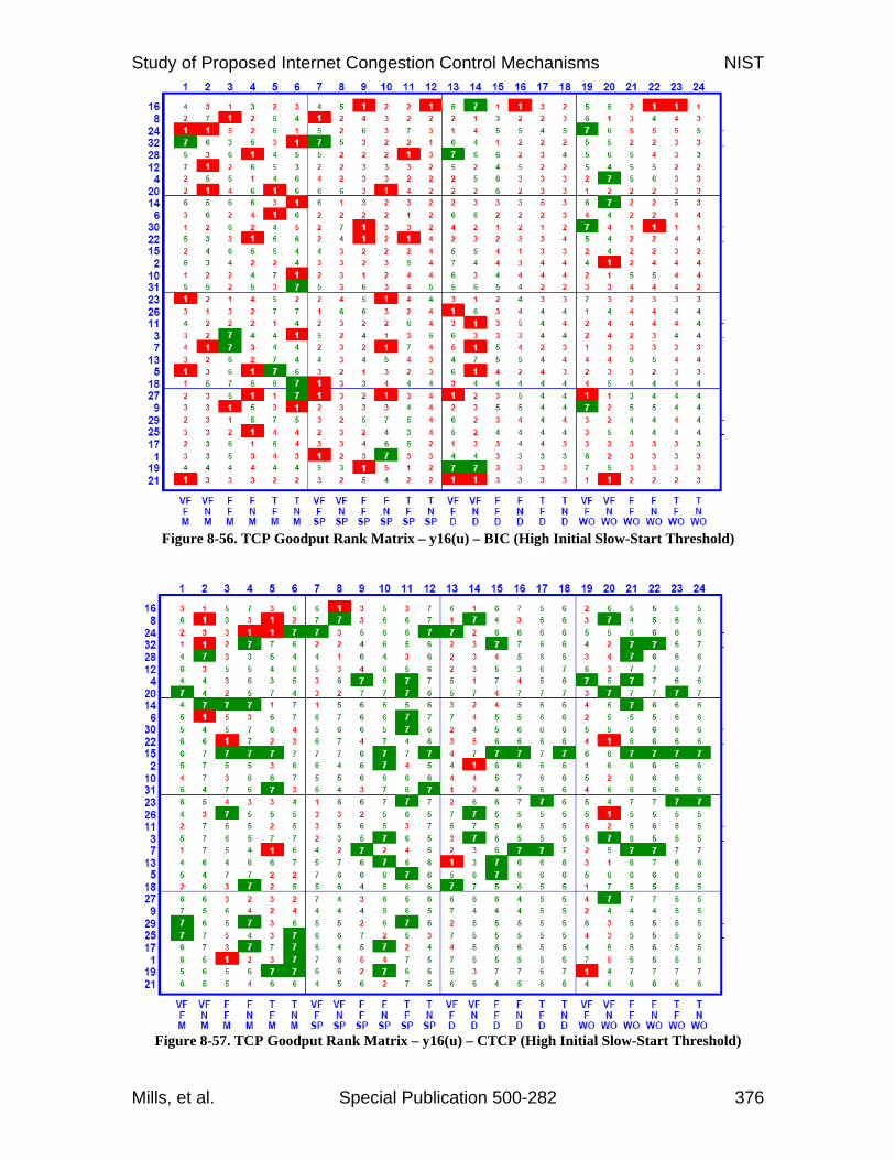
Study of Proposed Internet Congestion Control Mechanisms NIST
Mills, et al. Special Publication 500-282 376
Figure 8-56. TCP Goodput Rank Matrix – y16(u) – BIC (High Initial Slow-Start Threshold)
Figure 8-57. TCP Goodput Rank Matrix – y16(u) – CTCP (High Initial Slow-Start Threshold)

Study of Proposed Internet Congestion Control Mechanisms NIST
Mills, et al. Special Publication 500-282 377
Figure 8-58. TCP Goodput Rank Matrix – y16(u) – FAST (High Initial Slow-Start Threshold)
Figure 8-59. TCP Goodput Rank Matrix – y16(u) – FAST-AT (High Initial Slow-Start Threshold)

Study of Proposed Internet Congestion Control Mechanisms NIST
Mills, et al. Special Publication 500-282 378
Figure 8-60. TCP Goodput Rank Matrix – y16(u) – HSTCP (High Initial Slow-Start Threshold)
Figure 8-61. TCP Goodput Rank Matrix – y16(u) – HTCP (High Initial Slow-Start Threshold)
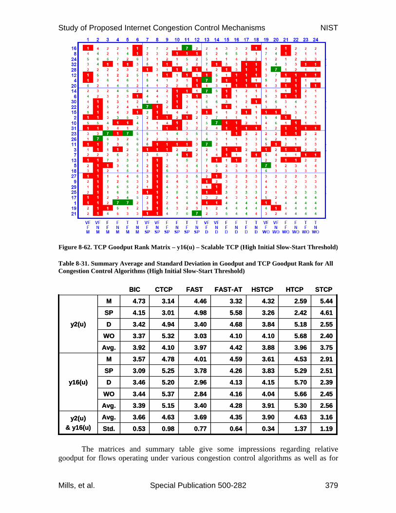
Study of Proposed Internet Congestion Control Mechanisms NIST
Mills, et al. Special Publication 500-282 379
Figure 8-62. TCP Goodput Rank Matrix – y16(u) – Scalable TCP (High Initial Slow-Start Threshold)
Table 8-31. Summary Average and Standard Deviation in Goodput and TCP Goodput Rank for All Congestion Control Algorithms (High Initial Slow-Start Threshold)
The matrices and summary table give some impressions regarding relative goodput for flows operating under various congestion control algorithms as well as for
1.191.370.340.640.770.980.53Std.
3.164.633.904.353.694.633.66Avg.y2(u) & y16(u)
2.565.303.914.283.405.153.39Avg.
2.455.664.044.162.845.373.44WO
2.395.704.154.132.965.203.46D
2.515.293.834.263.785.253.09SP
2.914.533.614.594.014.783.57M
y16(u)
3.753.963.884.423.974.103.92Avg.
2.405.684.104.103.035.323.37WO
2.555.183.844.683.404.943.42D
4.612.423.265.584.983.014.15SP
5.442.594.323.324.463.144.73M
y2(u)
STCPHTCPHSTCPFAST-ATFASTCTCPBIC
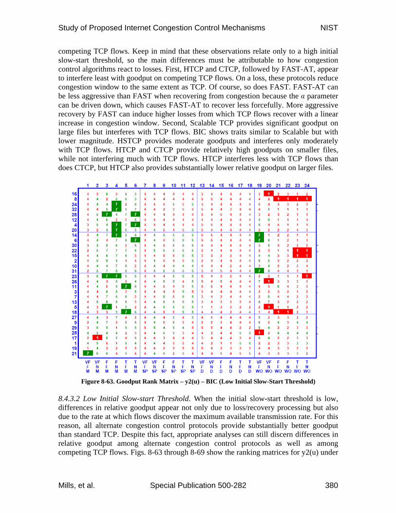
Study of Proposed Internet Congestion Control Mechanisms NIST
Mills, et al. Special Publication 500-282 380
competing TCP flows. Keep in mind that these observations relate only to a high initial slow-start threshold, so the main differences must be attributable to how congestion control algorithms react to losses. First, HTCP and CTCP, followed by FAST-AT, appear to interfere least with goodput on competing TCP flows. On a loss, these protocols reduce congestion window to the same extent as TCP. Of course, so does FAST. FAST-AT can be less aggressive than FAST when recovering from congestion because the parameter can be driven down, which causes FAST-AT to recover less forcefully. More aggressive recovery by FAST can induce higher losses from which TCP flows recover with a linear increase in congestion window. Second, Scalable TCP provides significant goodput on large files but interferes with TCP flows. BIC shows traits similar to Scalable but with lower magnitude. HSTCP provides moderate goodputs and interferes only moderately with TCP flows. HTCP and CTCP provide relatively high goodputs on smaller files, while not interfering much with TCP flows. HTCP interferes less with TCP flows than does CTCP, but HTCP also provides substantially lower relative goodput on larger files.
Figure 8-63. Goodput Rank Matrix – y2(u) – BIC (Low Initial Slow-Start Threshold)
8.4.3.2 Low Initial Slow-start Threshold. When the initial slow-start threshold is low, differences in relative goodput appear not only due to loss/recovery processing but also due to the rate at which flows discover the maximum available transmission rate. For this reason, all alternate congestion control protocols provide substantially better goodput than standard TCP. Despite this fact, appropriate analyses can still discern differences in relative goodput among alternate congestion control protocols as well as among competing TCP flows. Figs. 8-63 through 8-69 show the ranking matrices for y2(u) under

Study of Proposed Internet Congestion Control Mechanisms NIST
Mills, et al. Special Publication 500-282 381
a low initial slow-start threshold. The related matrices for y16(u) are given in Figs. 8-70 through 8-76. Table 8-32 summarizes the rankings.
Figure 8-64. Goodput Rank Matrix – y2(u) – CTCP (Low Initial Slow-Start Threshold)
Figure 8-65. Goodput Rank Matrix – y2(u) – FAST (Low Initial Slow-Start Threshold)
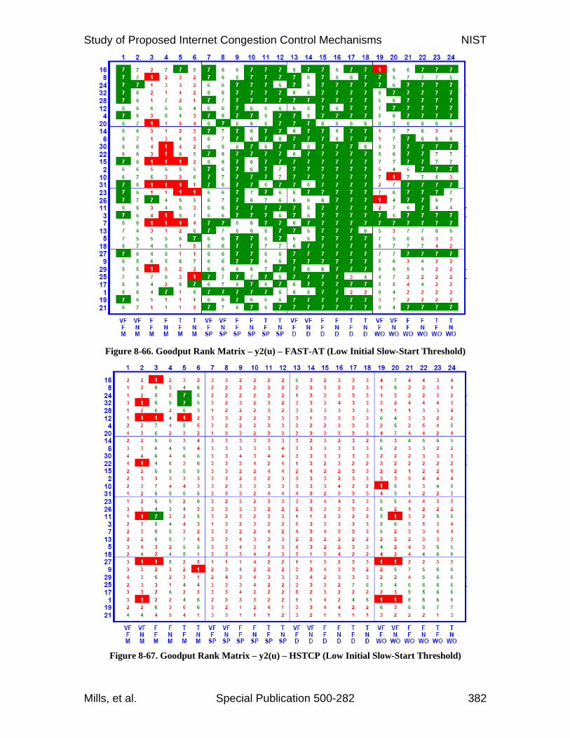
Study of Proposed Internet Congestion Control Mechanisms NIST
Mills, et al. Special Publication 500-282 382
Figure 8-66. Goodput Rank Matrix – y2(u) – FAST-AT (Low Initial Slow-Start Threshold)
Figure 8-67. Goodput Rank Matrix – y2(u) – HSTCP (Low Initial Slow-Start Threshold)
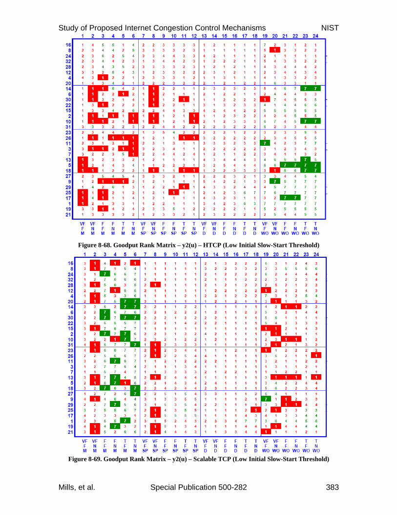
Study of Proposed Internet Congestion Control Mechanisms NIST
Mills, et al. Special Publication 500-282 383
Figure 8-68. Goodput Rank Matrix – y2(u) – HTCP (Low Initial Slow-Start Threshold)
Figure 8-69. Goodput Rank Matrix – y2(u) – Scalable TCP (Low Initial Slow-Start Threshold)
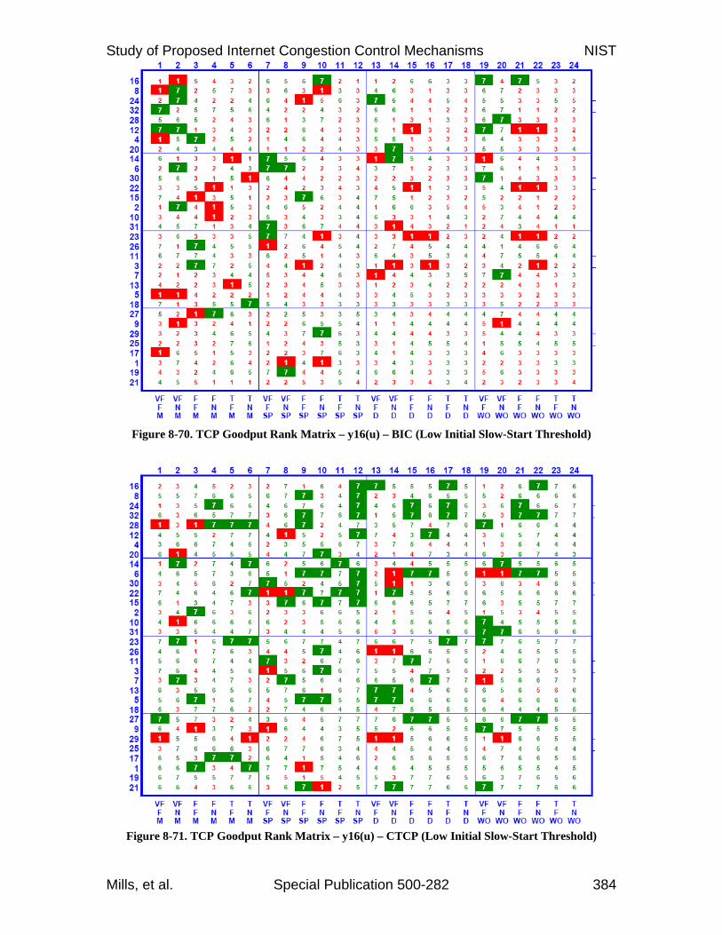
Study of Proposed Internet Congestion Control Mechanisms NIST
Mills, et al. Special Publication 500-282 384
Figure 8-70. TCP Goodput Rank Matrix – y16(u) – BIC (Low Initial Slow-Start Threshold)
Figure 8-71. TCP Goodput Rank Matrix – y16(u) – CTCP (Low Initial Slow-Start Threshold)
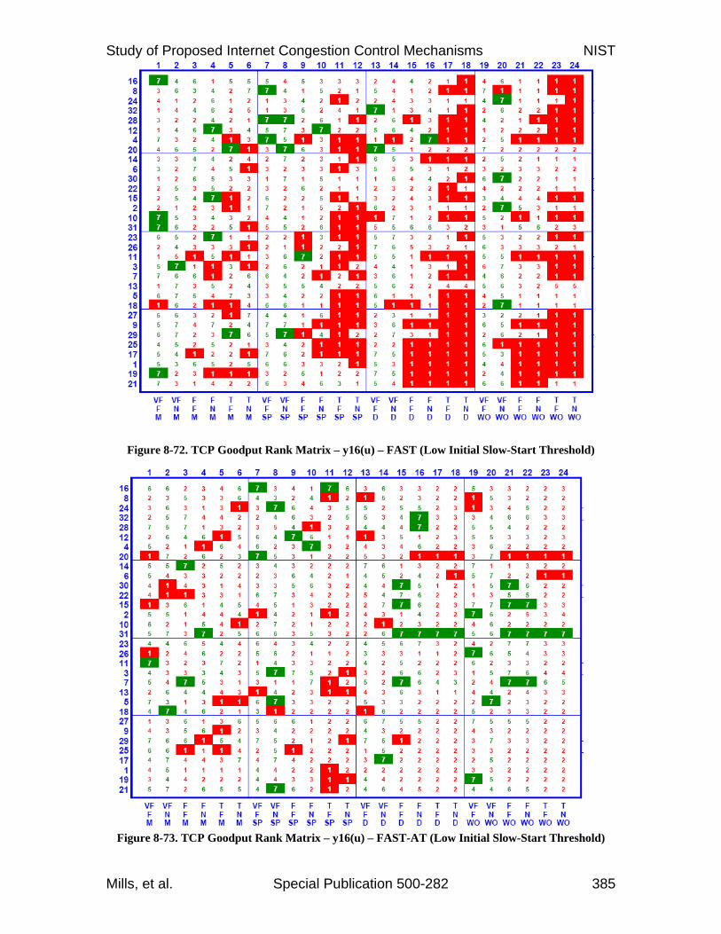
Study of Proposed Internet Congestion Control Mechanisms NIST
Mills, et al. Special Publication 500-282 385
Figure 8-72. TCP Goodput Rank Matrix – y16(u) – FAST (Low Initial Slow-Start Threshold)
Figure 8-73. TCP Goodput Rank Matrix – y16(u) – FAST-AT (Low Initial Slow-Start Threshold)
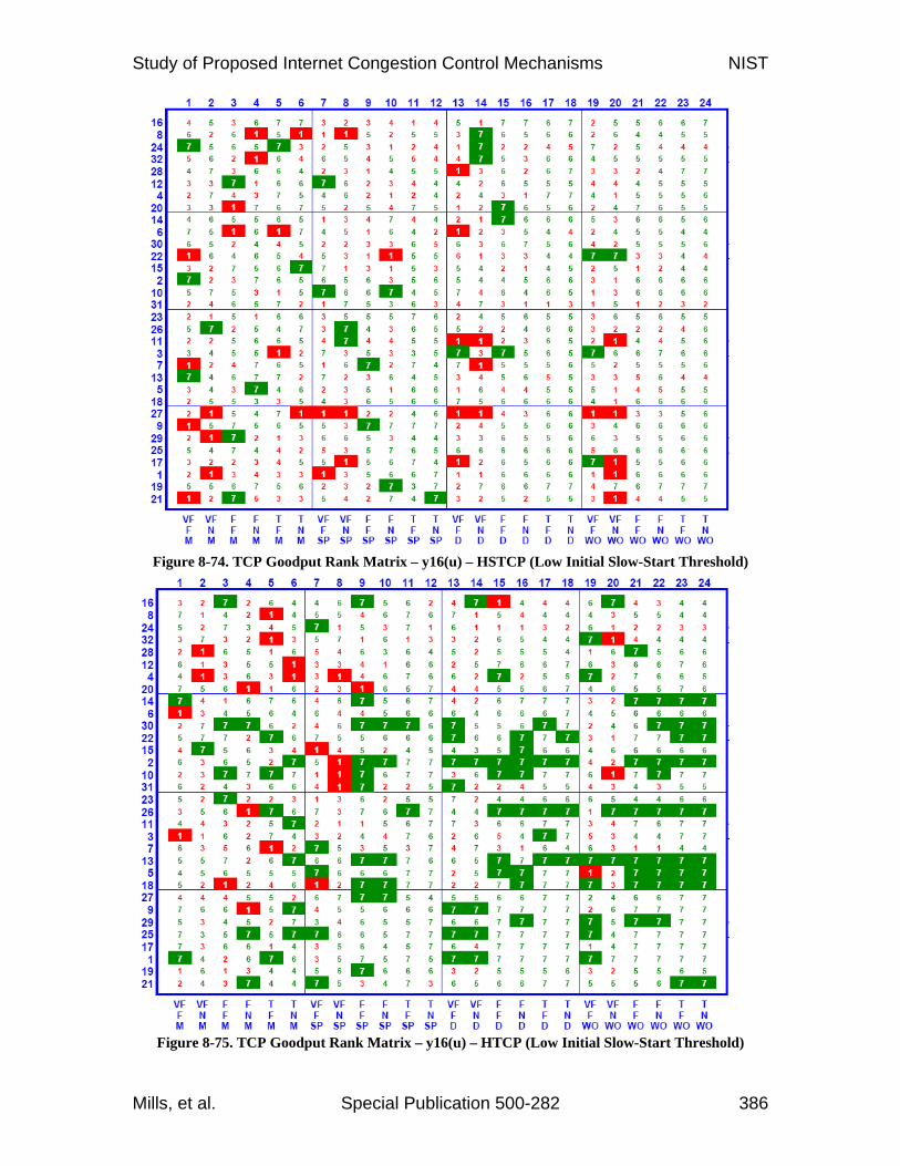
Study of Proposed Internet Congestion Control Mechanisms NIST
Mills, et al. Special Publication 500-282 386
Figure 8-74. TCP Goodput Rank Matrix – y16(u) – HSTCP (Low Initial Slow-Start Threshold)
Figure 8-75. TCP Goodput Rank Matrix – y16(u) – HTCP (Low Initial Slow-Start Threshold)

Study of Proposed Internet Congestion Control Mechanisms NIST
Mills, et al. Special Publication 500-282 387
Figure 8-76. TCP Goodput Rank Matrix – y16(u) – Scalable TCP (Low Initial Slow-Start Threshold)
Table 8-32. Summary Average and Standard Deviation in Goodput and TCP Goodput Rank for All Congestion Control Algorithms (Low Initial Slow-Start Threshold)
Figs. 8-63 through 8-76 and Table 8-32 reveal the key differences in relative goodput, under low initial slow-start threshold, among flows using alternate congestion
0.971.470.751.471.600.550.59Std.
3.213.873.754.604.234.643.71Avg.y2(u) & y16(u)
3.755.044.393.412.845.043.52Avg.
3.565.354.513.502.405.183.50WO
3.795.474.523.292.545.113.28D
3.975.024.233.202.894.983.71SP
3.684.324.323.643.544.903.61M
y16(u)
2.662.703.115.795.614.243.89Avg.
2.554.283.545.584.684.632.74WO
1.612.212.796.706.114.743.85D
2.161.942.666.586.423.894.36SP
4.322.363.464.315.243.704.60M
y2(u)
STCPHTCPHSTCPFAST-ATFASTCTCPBIC
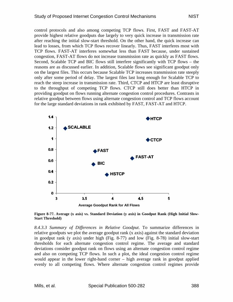
Study of Proposed Internet Congestion Control Mechanisms NIST
Mills, et al. Special Publication 500-282 388
control protocols and also among competing TCP flows. First, FAST and FAST-AT provide highest relative goodputs due largely to very quick increase in transmission rate after reaching the initial slow-start threshold. On the other hand, the quick increase can lead to losses, from which TCP flows recover linearly. Thus, FAST interferes most with TCP flows. FAST-AT interferes somewhat less than FAST because, under sustained congestion, FAST-AT flows do not increase transmission rate as quickly as FAST flows. Second, Scalable TCP and BIC flows still interfere significantly with TCP flows – the reasons are as discussed earlier. In addition, Scalable flows see significant goodput only on the largest files. This occurs because Scalable TCP increases transmission rate steeply only after some period of delay. The largest files last long enough for Scalable TCP to reach the steep increase in transmission rate. Third, CTCP and HTCP are least disruptive to the throughput of competing TCP flows. CTCP still does better than HTCP in providing goodput on flows running alternate congestion control procedures. Contrasts in relative goodput between flows using alternate congestion control and TCP flows account for the large standard deviations in rank exhibited by FAST, FAST-AT and HTCP. Figure 8-77. Average (x axis) vs. Standard Deviation (y axis) in Goodput Rank (High Initial Slow-Start Threshold)
8.4.3.3 Summary of Differences in Relative Goodput. To summarize differences in relative goodputs we plot the average goodput rank (x axis) against the standard deviation in goodput rank (y axis) under high (Fig. 8-77) and low (Fig. 8-78) initial slow-start thresholds for each alternate congestion control regime. The average and standard deviations consider goodput rank on flows using an alternate congestion control regime and also on competing TCP flows. In such a plot, the ideal congestion control regime would appear in the lower right-hand corner – high average rank in goodput applied evenly to all competing flows. Where alternate congestion control regimes provide
HTCP
CTCP
FAST-AT
Average Goodput Rank for All Flows
FAST
HSTCP
BIC
SCALABLE
HTCP
CTCP
FAST-AT
Average Goodput Rank for All Flows
FAST
HSTCP
BIC
SCALABLE

Study of Proposed Internet Congestion Control Mechanisms NIST
Mills, et al. Special Publication 500-282 389
equally high average rankings, one should prefer the regime with lower standard deviation in rank.
Figure 8-78. Average vs. Standard Deviation in Goodput Rank (Low Initial Slow-Start Threshold)
Fig. 8-77 and 8-78 show CTCP to be best with respect to relative goodput rank. CTCP provides the highest average rank (over 4.5) and the lowest standard deviation among high ranking alternatives (e.g., HTCP in Fig. 8-77 and FAST-AT in Fig. 8-78). Further, Scalable TCP is worst with respect to relative goodput rank and BIC is second worst. HSTCP ranks in the middle. HTCP ranks well with respect to average goodput under large initial slow-start threshold, but ranks significantly less well under low initial slow-start threshold. Further, HTCP exhibits a high standard deviation, interfering relatively little with TCP flows, while underperforming other alternate congestion control algorithms with respect to large files. The relative performance of FAST-AT might be considered second best, though due to its rapid increase in transmission rate (under low initial slow-start threshold) FAST-AT can induce losses in TCP flows, which recover only linearly. FAST induces more losses in TCP flows than FAST-AT, and also benefits from the same (as FAST-AT) rapid increase in transmission rate when the initial slow-start threshold is low.
8.5 Findings This experiment considered a range of files sizes (movies, service packs, documents and Web objects) being transferred across a relatively uncongested network, where some (fast and typical) paths experienced more congestion than others (very fast paths) and where some flows could achieve a maximum rate of 80 x 103 pps, while others were constrained (by the interface speed of a sender or receiver) to at most 8 x 10³ pps. Flows using TCP congestion control were mixed with flows using one of seven alternate congestion control
HTCP
CTCP
FAST-AT
Average Goodput Rank for All Flows
FAST
HSTCP
BIC
SCALABLE
HTCP
CTCP
FAST-AT
Average Goodput Rank for All Flows
FAST
HSTCP
BIC
SCALABLE
Study of Proposed Internet Congestion Control Mechanisms NIST
Mills, et al. Special Publication 500-282 390
algorithms. In general, under these conditions, goodput experienced on flows is influenced by three main factors (when ignoring network speed and delay): (1) quickeness with which the maximum transfer rate is achieved, (2) file size and (3) packet losses and related recovery procedures. The 32 conditions simulated in this experiment were run twice: once with a high and once with a low initial slow-start threshold. Under a high threshold, all flows used the same algorithm (limited slow-start) to find the maximum transfer rate. In such cases, only file size and packet loss/recovery procedures served to distinguish goodput among the various algorithms investigated. Under a low threshold, flows discovered the maximum transfer rate using techniques associated with the specific algorithms. In such cases, the quickness with which a flow could reach maximum transfer rate is the largest factor distinguishing among goodput.
8.5.1 Finding #1 Under low congestion, choice of initial slow-start threshold significantly influenced goodput differences between TCP flows and flows running alternate congestion control algorithms. Given a high threshold, all flows discovered the maximum available transmission rate using the same slow-start algorithm. In such cases, goodput differences between TCP flows and flows running alternate algorithms were diminished greatly, depending only on differences associated with loss/recovery procedures. Loss/recovery procedures played a larger role with bigger files (more packets mean more losses) and in congested areas and conditions (more simultaneous flows lead to more losses). Given a low threshold, all alternate algorithms yielded superior performance to standard TCP due to TCP’s linear rate of increase in transmission toward the maximum rate. FAST and FAST-AT, which showed the quickest increase to the maximum transmission rate, benefited most from a low initial slow-start threshold and exhibited significantly higher goodputs (than the other algorithms) for all but the smallest files. CTCP achieved the second fastest pace of increase to maximum rate.
8.5.2 Finding #2 With increasing losses, due to large file size or path congestion, goodputs were distinguished mainly by loss/recovery procedures. Scalable TCP, BIC and HSTCP do not decrease their transmission rate as much as the other algorithms when a loss is detected. This means that already established flows continue to transmit at higher rates, inducing losses in newer flows, and also in ongoing TCP flows, which cut their transmission rate in half on each loss. Thus, under congested conditions, Scalable TCP, BIC and HSTCP interfered most with competing TCP flows. On the other hand, FAST, FAST-AT, CTCP and HTCP reduce transmission rate by half on a loss, which mirrors the reduction of TCP flows. Of course, FAST (and sometimes FAST-AT) subsequently increases transmission rate quickly to recover from the loss, while CTCP increases transmission rate second most quickly. HTCP delays for one second without another packet loss before increasing transmission rate more than linearly, so HTCP lagged somewhat in recovering from losses.
The ability of FAST to rapidly increase transmission rate on loss recovery was somewhat of a double-edged sword. Increased rate of transmission by competing FAST flows could induce additional losses in TCP flows, which recover at only a linear rate. Thus, under such circumstances, FAST could interfere markedly with TCP flows. FAST-
Study of Proposed Internet Congestion Control Mechanisms NIST
Mills, et al. Special Publication 500-282 391
AT includes the ability to reduce the parameter, so when congestion is significant FAST-AT flows recover less aggressively than FAST flows. For this reason, FAST-AT interfered somewhat less with standard TCP flows.
8.5.3 Finding #3 Overall, CTCP provided the best balance in relative goodput achieved on all flows. CTCP interfered little (but HTCP interfered least) with TCP flows and proved second best (after FAST/FAST-AT) at providing goodput to flows using alternate congestion control procedures. FAST-AT disrupted TCP flows somewhat more than HTCP and CTCP, while providing nearly the best goodput to flows using alternate procedures.
8.5.4 Finding #4 As seen in earlier experiments, this experiment showed that use of some alternate congestion control protocols altered selected macroscopic characteristics of the network. Here, however, the characteristic changes were, in general, not statistically significant. We attribute this to two main factors: (1) overall congestion levels were kept much lower than in previous experiments (e.g., Chapters 6 and 7) and (2) FAST and FAST-AT, which have similar characteristics, where not separated in the analyses, which (as discussed in Chapter 7) tended to reduce the statistical significance that might be attributed to either algorithm considered without the other. In general, the current experiments confirmed (as seen previously in Chapters 6 and 7) that FAST and FAST-AT tend to increase retransmission rate under higher congestion. Thus, more flows are pending in the connecting state and fewer flows complete per unit of time. In addition, Scalable TCP tends to increase buffer occupancy throughout the network. As discussed in Sec. 8.4.1, this can also lead to higher losses and increased retransmission rates, to more flows pending in the connecting state and to fewer flows completing per unit time. At lower congestion levels, Scalable TCP performed worse on these metrics than FAST. At higher congestion levels, FAST performed worse. Finally, we found again in this experiment that CTCP can exhibit a much higher average congestion window size than other congestion control algorithms. The increase appears more prominent under lower levels of congestion.
8.6 Conclusions In this section, we described an experiment to investigate effects on macroscopic behavior and user experience when deploying various congestion control algorithms in a simulated, heterogeneous network, i.e., a network that includes flows operating under normal TCP congestion control procedures together with flows operating under one of seven alternate congestion control algorithms. Mixing each alternate congestion control regime together with standard TCP enabled us to investigate the influence of alternate congestion avoidance algorithms on the performance of TCP flows, as might prove important during a period of transition from TCP toward adoption of an alternate congestion control regime. Under half of the test conditions more flows operated with TCP, as might be typical in earlier stages of transition to an alternate congestion control regime, while under the remaining test conditions more flows operated with an alternate congestion control regime, as might be typical in later stages of transition. We also introduced additional flow sizes to represent downloading movies and software service
Study of Proposed Internet Congestion Control Mechanisms NIST
Mills, et al. Special Publication 500-282 392
packs. These file sizes augmented the Web objects and document downloads used in previous experiments. We adopted a small-scale network because earlier experiments suggested that a small network yields significant information while requiring fewer resources. Reducing computational cost allowed us to repeat our experiments first with a high initial slow-start threshold and then with a low initial slow-start threshold. We took this step in light of the apparent significance of the initial slow-start threshold, as uncovered in earlier experiments (Chapters 6 and 7).
We demonstrated that, under the conditions simulated, and setting aside network speed and delay, goodput experienced on flows is influenced by three main factors: (1) quickness with which the maximum transfer rate is achieved, (2) file size and (3) packet losses and related recovery procedures. We showed that adopting a high initial slow-start threshold throughout the network allowed all flows to reach maximum transfer rate at the same speed, which substantially reduced goodput differences among TCP flows and flows using alternate congestion control algorithms. With a high threshold, only loss/recovery procedures distinguished goodput among congestion control algorithms. We found that on a loss, Scalable TCP, BIC and HSTCP reduced transmission rate less than other algorithms, causing Scalable TCP, BIC and HSTCP to interfere more with TCP flows under congested conditions. While CTCP, FAST and FAST-AT (and sometimes HTCP) halved their transmission rate on a loss, FAST (and sometimes FAST-AT) where able to increase transmission rate at the quickest pace, followed by CTCP. The pace of increase of HTCP was much less. Under heavy congestion, FAST-AT was less aggressive in recovering from losses than was FAST.
We showed that under a low initial slow-start threshold all of the alternate congestion control algorithms reached the maximum transmission rate much more quickly than TCP, which was limited to a linear rate of increase. FAST (and FAST-AT) increased transmission rate most quickly, followed by CTCP. Scalable TCP increased transmission rate least quickly during a flow’s initial period before achieving a steep rate of increase, so under a low initial slow-start threshold, Scalable achieved substantial goodputs only on large files. Differences in the speed of increase in transmission rate among the other congestion control algorithms (BIC, HSTCP and HTCP) did not appear significant. We found that CTCP gave the best balance in goodput among all flows, but FAST and FAST-AT flows achieved the highest goodputs when all flows used a low initial slow-start threshold.
We were also able to confirm some network-wide results from earlier experiments, where FAST and FAST-AT exhibited higher retransmission rates, more pending flow connections and fewer flows completing. In addition, we found that, under high initial slow-start threshold, Scalable TCP could also exhibit such undesirable network-wide properties.
In the next section, we revisit the results from this section by rerunning the experiment on a larger (10 times more sources) and faster (10 times higher capacity) network. The substantial increase in computational requirements arising from this increase in network size and speed will limit us to consider only one setting for initial slow-start threshold. We chose the high initial slow-start threshold in order to focus on differences in loss/recovery processing. We expect that the larger network will experience substantially less congestion under most conditions. Given the findings from the current section, we suspect a less congested network, where all flows use a high

Study of Proposed Internet Congestion Control Mechanisms NIST
Mills, et al. Special Publication 500-282 393
initial slow-start threshold, will yield a narrowing of differences in goodput among the alternate congestion control algorithms. Fewer losses should mean that the algorithms have fewer opportunities to invoke their loss/recovery behaviors.