chapter 7leeds-faculty.colorado.edu/roca4364/misc/fnce4030_files/...chapter 7 optimal risky...

INVESTMENTS | BODIE, KANE, MARCUS

Copyright © 2011 by The McGraw-Hill Companies, Inc. All rights reserved. McGraw-Hill/Irwin

CHAPTER 7

Optimal Risky Portfolios


7-2

The Investment Decision

• Top-down process with 3 steps:

1.Capital allocation between the risky portfolio

and risk-free asset

2.Asset allocation across broad asset classes

3.Security selection of individual assets within

each asset class


7-3

Diversification and Portfolio Risk

• Market risk

– Systematic or nondiversifiable

• Firm-specific risk

– Diversifiable or nonsystematic


7-4

Figure 7.1 Portfolio Risk as a Function of the Number of Stocks in the Portfolio


7-5

Figure 7.2 Portfolio Diversification


7-6

Covariance and Correlation

• Portfolio risk depends on the

correlation between the returns of the

assets in the portfolio

• Covariance and the correlation

coefficient provide a measure of the

way returns of two assets vary


7-7

Two-Security Portfolio: Return

Portfolio Return

Bond Weight

Bond Return

Equity Weight

Equity Return

p D ED E

P

D

D

E

E

r

r

w

r

w

r

w wr r

( ) ( ) ( )p D D E EE r w E r w E r


7-8

Two-Security Portfolio: Risk

EDEDEEDD rrCovwwww ,222222

p

= Variance of Security D

= Variance of Security E

= Covariance of returns for

Security D and Security E

2

E

2

D

ED rrCov ,


7-9

Two-Security Portfolio: Risk

• Another way to express variance of the

portfolio is to think of Covariances:

EDED

EEEE

DDDD

rrCovww

rrCovww

rrCovww

,2

,

,2

p


7-10

D,E = Correlation coefficient of

returns

D = Standard deviation of

returns for Security D

E = Standard deviation of

returns for Security E

Covariance

EDDEED rrCov ,


7-11

Table 7.2 Computation of Portfolio Variance From the Covariance Matrix


7-12

A portfolio of 3 Assets

1 1 2 2 3 3( ) ( ) ( ) ( )pE r w E r w E r w E r

• You have three assets with weights

w1, w2, w3

• The portfolio return is simply the linear

combination of the returns with same

coefficients:

Q. is the portfolio’s variance also the

linear combination of the 3 variances?


Bordered Matrix for 3 Assets

w1 w2 w3

w1 Cov(1,1) Cov(1,2) Cov(1,3)

w2 Cov(2,1) Cov(2,2) Cov(2,3)

w3 Cov(3,1) Cov(3,2) Cov(3,3)

7-13

Step 1: write the covariance matrix and its weights



w1 w2 w3

w1

w2

w3

7-14

Step 2: Symmetry! baabCovbaCov ,,,

2

1 2,1 3,1

2

2

2

3

3,2

3,1 3,2

2,1


w1 w2 w3

w1

w2

w3


7-15

Step 3: multiply by the weights around the border

2

1w

2

2w

2

3w

21ww

21ww

31ww

31ww

32ww

32ww

2

1 2,1 3,1

2

2

2

3

3,2

3,1 3,2

2,1


7-16


3,2323,1312,121

2

3

2

3

2

2

2

2

2

1

2

1

2

222

wwwwww

wwwp

Covariance terms

Step 4: add-up all the pieces

Remember bababa ,,



w1 w2 w3

w1

w2

w3

7-17

All in one step

2

1 212,1 313,1

2

2

2

3

323,2

313,1 323,2

212,1

2

1w

2

2w

2

3w

31ww

33ww

21ww

33ww31ww

21ww


7-18


323,232

313,131

212,121

2

3

2

3

2

2

2

2

2

1

2

1

2

2

2

2

ww

ww

ww

wwwp

Add-up all the pieces


7-19

Range of values for correlation

+ 1.0 > > -1.0

If = 1.0, the securities are perfectly

positively correlated

If = - 1.0, the securities are perfectly

negatively correlated

Correlation Coefficients: Possible Values


7-20

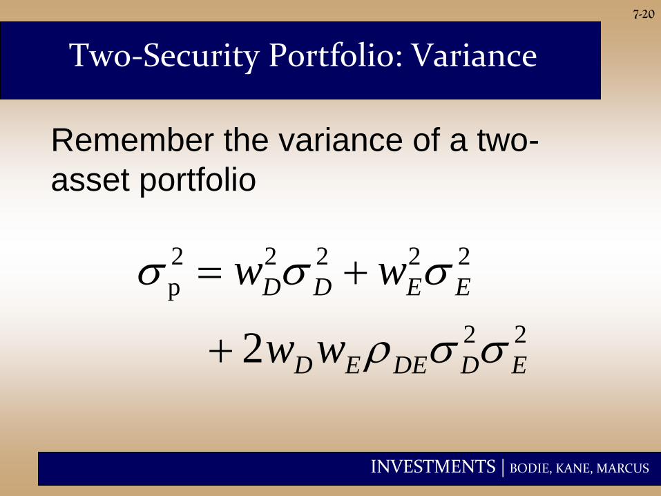
Two-Security Portfolio: Variance

Remember the variance of a two-

asset portfolio

22

22222

p

2 EDDEED

EEDD

ww

ww


7-21

Correlation Coefficients

• When ρDE = 1, there is no diversification

DDEEP ww

D

ED

DE

ED

ED www

1 and

0222222

p EDEDEEDD wwww

• When ρDE = -1, a perfect hedge is when:

the solution (which also makes wD+wE=1) is:


7-22

Figure 7.3 Portfolio Expected Return as a Function of Investment Proportions


7-23

Figure 7.4 Portfolio Standard Deviation as a Function of Investment Proportions


7-24

The Minimum Variance Portfolio

• The minimum variance portfolio is the portfolio composed of the risky assets that has the smallest standard deviation, the portfolio with least risk.

• If correlation < +1 the portfolio standard deviation may be smaller than that of either of the individual component assets.

• If correlation = -1 the standard deviation of the minimum variance portfolio is zero.


7-25

Figure 7.5 Portfolio Expected Return as a Function of Standard Deviation

Portfolio

opportunity

set for given


7-26

• The amount of possible risk reduction

through diversification depends on the

correlation.

• The risk reduction potential increases as

the correlation approaches -1.

– If = +1.0, no risk reduction is possible.

– If = 0, σP may be less than the standard

deviation of either component asset.

– If = -1.0, a riskless hedge is possible.

Correlation Effects


7-27

Figure 7.6 The Opportunity Set of the Debt and Equity Funds and Two Feasible CALs


7-28

The Sharpe Ratio

• Maximize the slope of the CAL for any

possible portfolio, P.

• The objective function is the slope:

• The slope is also the Sharpe ratio.

( )P f

P

P

E r rS


7-29

Figure 7.7 The Opportunity Set of the Debt and Equity Funds with the Optimal CAL and the Optimal Risky Portfolio


7-30

Figure 7.8 Determination of the Optimal Overall Portfolio


7-31

Markowitz Portfolio Selection Model

• Security Selection

– The first step is to determine the risk-

return opportunities available.

– All portfolios that lie on the minimum-

variance frontier from the global

minimum-variance portfolio and upward

provide the best risk-return

combinations


7-32

Figure 7.10 The Minimum-Variance Frontier of Risky Assets


7-33


• We now search for the CAL with the

highest reward-to-variability ratio

• That means to find that optimal line

that stems from the risk-free point

and is tangent to the efficient frontier


7-34

Figure 7.11 The Efficient Frontier of Risky Assets with the Optimal CAL


7-35


• Everyone invests in P, regardless of their

degree of risk aversion.

– More risk averse investors put more in the

risk-free asset.

– Less risk averse investors put more in P.


7-36

Capital Allocation and the Separation Property

• The separation property tells us that the

portfolio choice problem may be

separated into two independent tasks:

– Determination of the optimal risky

portfolio is purely technical

– Allocation of the complete portfolio to T-

bills versus the risky portfolio depends

on personal preference.


7-37

Figure 7.13 Capital Allocation Lines with Various Portfolios from the Efficient Set


7-38

The Power of Diversification

• Remember:

• If we define the average variance and average

covariance of the securities as:

2

1 1

( , )n n

P i j i j

i j

w w Cov r r

2 2

1

1 1

1

1( , )

( 1)

n

i

i

n n

i j

j ij i

n

Cov Cov r rn n


7-39

The Power of Diversification

• We can then express portfolio variance as:

2 21 1P

nCov

n n


7-40

Table 7.4 Risk Reduction of Equally Weighted Portfolios in Correlated and Uncorrelated Universes


7-41

Optimal Portfolios and Nonnormal Returns

• Fat-tailed distributions can result in extreme

values of VaR and ES and encourage smaller

allocations to the risky portfolio.

• If other portfolios provide sufficiently better VaR

and ES values than the mean-variance efficient

portfolio, we may prefer these when faced with

fat-tailed distributions.


7-42

Risk Pooling and the Insurance Principle

• Risk pooling: merging uncorrelated, risky

projects as a means to reduce risk.

– increases the scale of the risky investment by

adding additional uncorrelated assets.

• The insurance principle: risk increases less than

proportionally to the number of policies insured

when the policies are uncorrelated

– Sharpe ratio increases


7-43

Risk Sharing

• As risky assets are added to the portfolio, a

portion of the pool is sold to maintain a risky

portfolio of fixed size.

• Risk sharing combined with risk pooling is the

key to the insurance industry.

• True diversification means spreading a portfolio

of fixed size across many assets, not merely

adding more risky bets to an ever-growing risky

portfolio.


7-44

Investment for the Long Run

Long Term Strategy

• Invest in the risky portfolio for 2 years.

– Long-term strategy is riskier.

– Risk can be reduced by selling some of the risky assets in year 2.

– “Time diversification” is not true diversification.

Short Term Strategy

• Invest in the risky

portfolio for 1 year and

in the risk-free asset for

the second year.

chapter 7leeds-faculty.colorado.edu/roca4364/misc/fnce4030_files/...chapter 7 optimal risky...

Documents