chapter 7 ratio and financial statement · pdf file1 chapter 7 ratio and financial statement...

1

Chapter 7 Ratio and Financial Statement Analysis

The objectives of this chapter are to enable you to:

Compute and categorize ratios

Apply ratio analysis to evaluate a company’s liquidity, performance and risks

Construct and analyze common-size accounting statements

Be wary of potential pitfalls undermining ratio and financial statement analysis

A. Introduction to Financial Statement Analysis

Financial statement analysis will usually involve the comparison of financial statement

figures based on either a cross-section of different firms or based on a time-series of statements.

Among the tools used by the analyst are common-size statements where income statement items

are expressed as a percentage of revenues and balance sheet items are expressed as a percentage

of assets. Standardizing statement balances enable simplified comparisons either across firms or

over time. Financial ratios are also most important and will be discussed in detail later. The

construction of pro-forma statements will also be discussed here.

There exist numerous sources for financial statement data. Data will be available from

publicly traded companies in annual reports or 10-K reports filed with the S.E.C. Standardized

hard copy (paper) statements may be purchased from companies such as Moody's, Standard and

Poors, Commerce Clearing House, Value Line and Dun and Bradstreet. Examples for sources of

such standardized reports include Moody's Handbook of Common Stocks, Value Line Investment

Survey, FactSet, StockVal, WRDS and Standard and Poor's Industry Survey. Computerized data

sources such as Yahoo.com, Compustat and CD Disclosure are available at many libraries and

can download data to computer-based spreadsheets. However, users should be aware that these

data bases (paper or computer) may exclude firms, particularly those no longer in existence, may

be missing recent data, may contain recording errors, may record statement accounts

inconsistently across firms and may altogether exclude important accounting statement items.

Some analysts are concerned with the distinction between value and growth stocks.

Growth stocks may be thought of as those with exceptional growth potential. Some analysts use

historical earnings or returns growth as the indicator for growth stocks. Presumably, stocks with

high historical rates of growth may be expected to realize higher growth rates in the future.

Value investors are concerned with the market price of the stock relative to some other indicator

of value such as book value. The book to market value of a stock is often taken as an indicator of

the relative value of the stock. Higher book to market value is perceived as indicating a good

buy.

Chapter 7

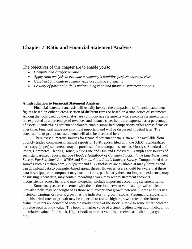
Common Size Accounting Statements

Firms use a variety of accounting conventions to present their financial statements,

rendering their comparisons somewhat more difficult. Analysts, newsletters and research

companies like Compustat restate financial statements in standardized form, making them easier

to compare. In addition, many analysts find common-size statements even easier to compare,

especially across firms or through time. Common-size income statements normally express all

items as a fraction or percentage of sales and common-size balance sheets normally express

balance sheet items as a fraction or percentage of assets. Income Statements and Balance Sheets

are presented for the Madison Company. Common-size statements for the Madison Company are

presented below the original statements.

Madison Company Cash Sales 2,000,000

Credit Sales 4,000,000 Total Sales 6,000,000

Other Revenue 1,000,000 Total Revenue 7,000,000

Raw Material cost 1,900,000

Direct Labor cost 1,100,000 Cost of Goods sold 3,000,000

Gross Margin 4,000,000

Plant operating cost 800,000

Maintenance cost 500,000

Managerial salaries 400,000

Other Fixed costs 300,000 Fixed Overhead cost 2,000,000

Depreciation 200,000 2,200,000

Earnings before interest and taxes ( EBIT) 1,800,000

Interest on current debt 50,000

Interest on notes payable 150,000

Interest on bonds payable 650,000

Total interest 850,000

Earnings Before taxes 950,000

Less Taxes @ 30 % of EBT 285,000 Net Income after taxes ( NIAT ) 665,000

Dividends 332,500

Retained Earnings 332,500

Number of shares outstanding 10,000

Earnings per share ( EPS ) 33

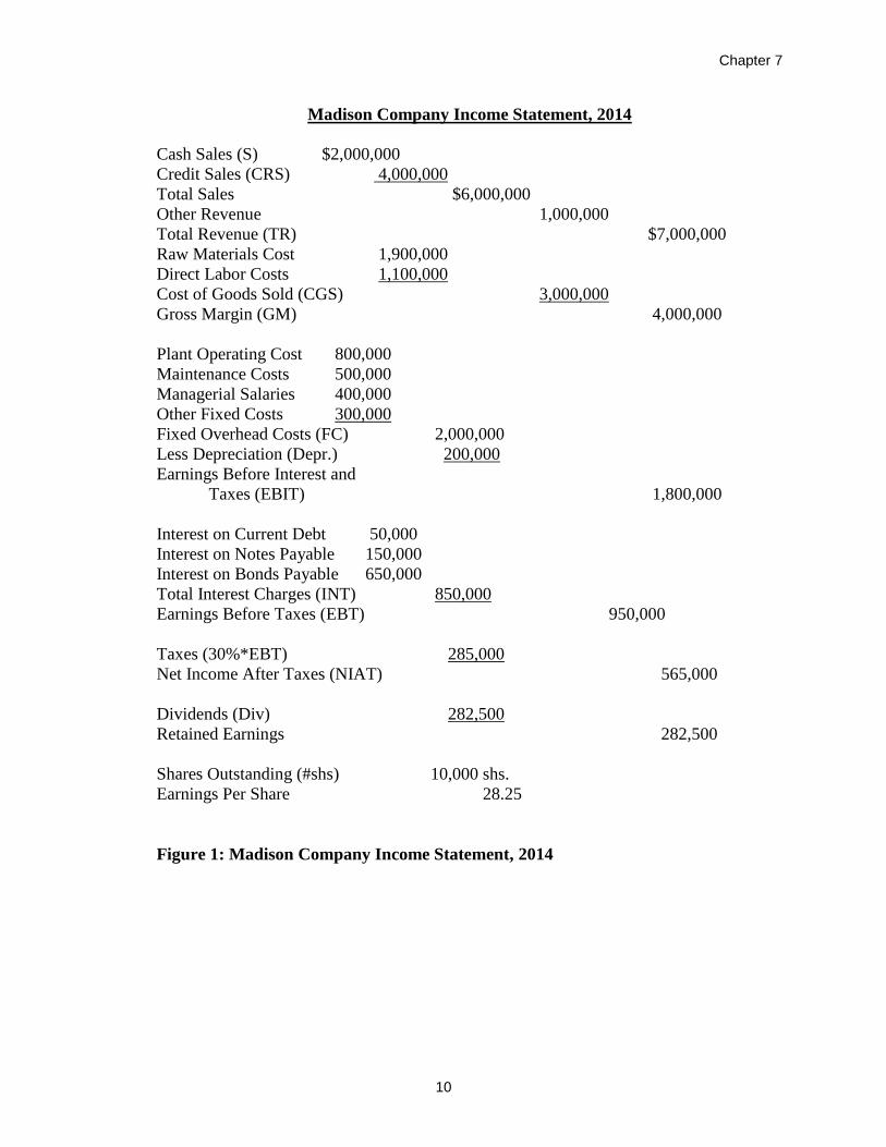
Figure 1: Madison Company Income Statement, 2014

MADISON COMPANY

Balance Sheet: December 31, 2013

Assets Amount Liabilities& Equity Amount

Cash $ 100,000 Accounts payable $ 500,000 Marketable Securities $ 300,000 Taxes payable $ 50,000 Inventory $ 700,000 Wages payable $ 50,000

Accounts Receivable $ 400,000

Current Assets $ 1,500,000 Current Liabilities $ 600,000 Equipment $ 200,000 Notes Payable $ 1,000,000 Plant $ 3,000,000 Bonds Payable $ 5,000,000

Land $ 4,000,000 Long Term Debt $ 6,000,000

Fixed Assets $ 7,200,000 Total Debt $ 6,600,000

Common Equity ( Par) $ 10,000

Cumulative Retained Earnings $ 2,090,000

Total Equity $ 2,100,000

Total Assets 8,700,000 Total Liabilities and Equity 8,700,000

Note:

Number of shares outstanding = 10,000

Market Price per share December 31, 2013 ( Po) = $ 250

Balance Sheet: December 31, 2014

Assets Amount Liabilities& Equity Amount

Cash $ 100,000 Accounts payable $ 500,000 Marketable Securities $ 300,000 Taxes payable $ 100,000 Inventory $ 500,000 Wages payable $ 50,000

Accounts Receivable $ 600,000

Current Assets $ 1,500,000 Current Liabilities $ 650,000 Equipment $ 900,000 Notes Payable $ 1,000,000 Plant $ 3,182,500 Bonds Payable $ 5,000,000

Land $ 3,500,000 Long Term Debt $ 6,000,000

Fixed Assets $ 7,582,500

Total Debt $ 6,650,000

Common Equity ( Par) $ 10,000

Cumulative Retained Earnings $ 2,422,500

Total Equity $ 2,432,500

Total Assets 9,082,500 Total Liabilities and Equity 9,082,500

Note:



Figure 2: Madison Company Balance Sheets

Chapter 8

MADISON COMPANY

Common Size Balance Sheet: December 31, 2013

Assets Liabilities& Equity

Cash 1.15 Accounts payable 5.75 Marketable Securities 3.45 Taxes payable 0.57 Inventory 8.05 Wages payable 0.57 Accounts Receivable 4.60

Current Assets 17.24 Current Liabilities 6.90

Equipment 2.30 Notes Payable 11.49 Plant 34.48 Bonds Payable 57.47 Land 45.98 Long Term Debt 68.97 Fixed Assets 82.76

Total Debt 75.86

Common Equity ( Par) 0.11

Cumulative Retained Earnings 24.02

Total Equity 24.14

Total Assets 100.00 Total Liabilities and Equity 100.00

Note:



Common Size Balance Sheet: December 31, 2014

Assets Liabilities& Equity

Cash 1.10 Accounts payable 5.51 Marketable Securities 3.30 Taxes payable 1.10 Inventory 5.51 Wages payable 0.55 Accounts Receivable 6.61

Current Assets 16.52 Current Liabilities 7.16

Equipment 9.91 Notes Payable 11.01 Plant 35.04 Bonds Payable 55.05 Land 38.54 Long Term Debt 66.06 Fixed Assets 83.48

Total Debt 73.22

Common Equity ( Par) 0.11

Cumulative Retained Earnings 26.67

Total Equity 26.78

Figure 3: Madison Company Common-Size Balance Sheets, 2013-14

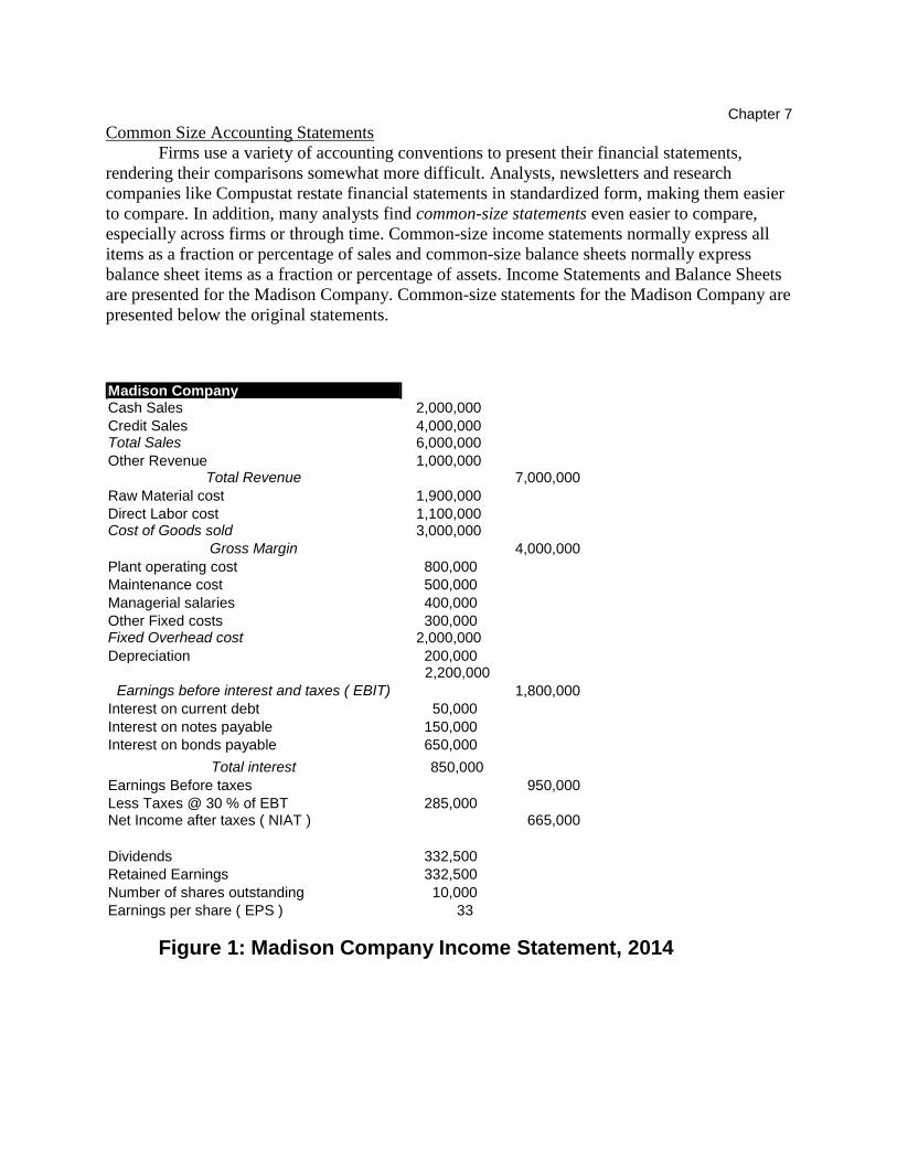
MadisonCompany

Income Statement for Year Ending 31 December, 2014 Common Size Income Statement

Cash Sales 29

Credit Sales 57

Total Sales 86

Other Revenue 14

Total Revenue 100

Raw Material cost 27

Direct Labor cost 16

Cost of Goods sold 43

Gross Margin 57

Plant operating cost 11

Maintenance cost 7

Managerial salaries 6

Other Fixed costs 4

Fixed Overhead cost 29

Depreciation 3

31

Earnings before interest and taxes ( EBIT) 26

Interest on current debt 1

Interest on notes payable 2

Interest on bonds payable 9

Total interest 12

Earnings Before taxes 14

Less Taxes @ 30 % of EBT 4

Net Income after taxes ( NIAT ) 10

Dividends 5

Retained Earnings 5

Figure 4: Madison Company Common-Size Income Statement, 2014

Chapter 7

6

B. Pro-forma Statements

A pro-forma statement is compiled based on forecasted or projected values. For example,

a pro-forma statement for 2015 compiled in 2014 lists accounts whose values were forecasted in

2014. The following portrays a historical balance sheet for 2014 along with a pro-forma balance

sheet for the Marlowe Company dated December 31, 2015 and a pro-forma income statement for

2015. Because one rarely predicts with certainty, account balances actually realized may differ

from the forecasted levels given in the pro-forma statements. Thus, the analyst may rely on a

combination of "best outcome", "worst outcome" and "most likely" outcome statements.

Computer based simulations and spreadsheets provide an efficient means of generating multiple

potential outcome scenarios.

The sales forecast might involve use of regression techniques along with analyses of

economy-wide and industry factors. The analyst must distinguish between variable and fixed

costs and determine the extent to which these costs are fixed or variable. Balance sheet and

income statement items must also reflect any capital investments and acquisitions projected by

the firm.

Marlowe Company Balance Sheet: Dec. 31, 2014

Assets Capital

Cash $77,703 Accounts Payable(AP) $90,000

Marketable Securities 15,000 Notes Payable 65,000

Accounts Receivable(AR) 50,000 Taxes Payable 15,000

Inventory (INV) 5,000 Current Liabilities(CL) 170,000

Current Assets(CA) $147,703

Term Loans 30,000

Land 7,000 Debentures 45,000

Plant (Net) 90,000 Total Debt(D) 245,000

Equipment (Net) 15,000

Fixed Assets(FA) $112,000 Common Equity Par 10,000

Total Assets $259,703 Paid in Capital 20,000

Retained Earnings -15,297

Total Equity (E) 14,703

Total Debt plus Equity $259,703

7

Pro-Forma Marlowe Company Income Statement, 2015 Sales (S) $295,000

Income from Securities (ifs) 1,500

Total Revenue (TR) 298,500 S + ifs

Beginning Inventory (bi) 5,000

Production Cost (pc) 175,000

Ending Inventory (ei) 8,000

Cost of Goods Sold (CGS) 172,000 bi + pc - ei

Gross Margin (GM) 116,500 TR - CGS

Fixed Manufacturing Cost (fmc) 70,000

Inventory Carry Cost (ic) 50

Selling and Administrative Costs (sc) 20,000

Depreciation - Plant (depr-p) 10,000

Depreciation - Machines (depr - m) 3,000

Depreciation - Other (depr -o) 400

Earnings Before Interest and Taxes (EBIT) 13,050 GM-fmc-ic-sc-DEPR

Note Payable Interest (int - n) 11,000

Term Loan Interest (int - t) 3,000

Debenture Interest (int - d) 4,500

Earnings Before Taxes (EBT) -5,450 EBIT - INT

Income Taxes (TAX) -2,507 EBT * .46

Net Income After Taxes (NIAT) -2,943 EBT - TAX

Dividends (DIV) 0

Add to Retained Earnings -2,943 NIAT – DIV

Pro-Forma Marlowe Company Balance Sheet: Dec. 31, 2015

Assets Capital

Cash $47,000 Accounts Payable(AP) $70,000

Marketable Securities 10,000 Notes Payable 55,000

Accounts Receivable(AR) 70,000 Taxes Payable 0

Inventory (INV) 8,000 Current Liabilities(CL) 125,000

Current Assets(CA) $135,000

Term Loans 42,240

Land 7,000 Debentures 55,000

Plant (Net) 80,000 Total Debt(D) 222,240

Equipment (Net) 12,000

Fixed Assets(FA) $99,000 Common Equity Par 10,000

Total Assets $234,000 Paid in Capital 20,000

Retained Earnings -18,240

Total Equity (E) 11,760

Total Debt plus Equity $234,000

Chapter 7

8

C. Ratio Analysis

Among the most important tools to fundamental analysts are accounting statement ratios.

This is because data taken from accounting statements are much more useful when they can be

compared to other data. This is the purpose of ratio analysis: to compare accounting statement

data. A financial ratio is simply one accounting statement value relative to another. Ratio

Analysis is very useful for measuring performance and risk and for comparing the relative

effectiveness of companies.

Figures 1 and 2 provide sample accounting statements for the Madison Company from

which ratios may be computed. Various ratios are listed and determined for the Madison

Company in Figures 3 and 4.

Ratios can be used to measure a number of important company characteristics. Various

ratios can be categorized according to which characteristics they are intended to measure. One

category of ratios is the liquidity group. These ratios are analyzed in an attempt to measure the

firm's liquidity position; that is, they are used to determine a firm's ability to convert assets into

cash in a short period of time. Firms must raise cash in order to operate. Even a firm that in the

past has been highly profitable will be unable to operate effectively if it is unable to raise cash to

compensate employees and to pay suppliers and taxes, etc. From Figure 3, we see that a sample

liquidity ratio is the firm's current ratio. This ratio, simply current assets divided by current

liabilities, may be used to measure a firm's ability to meet its short-run obligations. Current

Assets are those assets that are generally convertible into cash within a fairly short period of time

(frequently about one year). Cash, the most liquid of all assets and is likely to be a major

component of these current assets.

A second ratio group is the profitability ratios. These ratios are used to determine the

economic efficiency of the firm. An example of such a ratio is the firm's return-on-equity. This

ratio measures profits awarded to shareholders relative to how much they have invested in the

firm. A second profitability ratio is the firm's return-on-assets. This ratio measures cash flows

available to both shareholders and creditors compared to the total sum both have invested in the

firm. Thus, this ratio measures the profitability of all of the money invested in the firm.

A third ratio group comprises the leverage ratios. This group of ratios is used to

determine a firm's ability to meet its fixed obligations. These ratios are also very useful in

determining the risk or variability associated with a firm's profits. An obvious example of a

leverage ratio is the firm's debt-equity ratio. This ratio, simply the firm's debt level divided by its

equity level, measures the firm's ability to fulfill its obligations to creditors. Degree of Operating

Leverage and Degree of Financial Leverage ratios are very useful in the assessment of operating

and financial risk.

The fourth group discussed here are the activity ratios. These ratios measure a firm's

ability to perform certain activities. An example of such a ratio is the sales-turnover ratio. This

ratio measures a firm's capacity to sell its products given a specified level of investment.

The fifth group discussed in this chapter are the market ratios. These ratios, including P/E

and market-to-book ratios, focus on market values of shares or equity relative to certain

accounting statement values. These ratios are particularly useful for stock valuation.

Figures 1 and 2 display accounting statements for the Madison Company. A variety of

ratios for this company are computed in Figure 4. Ratios are defined and grouped in Figure 3.

The use of ratios requires some standards for comparison. Useful standards for

comparison include ratios generated by the firm in previous periods, ratios generated by other

firms and target levels set by the firm. Contrary to the beliefs of some individuals, there are no

9

target ratio levels (such as the 2 to 1 current ratio sometimes mentioned) that may be universally

applied across all firms in all situations. Often, the most difficult steps in ratio analysis are

generating appropriate standards for comparison and inferring reasons for deviation from those

standards.

Comparison of ratios across several time periods may provide useful information

regarding firm trends. For example, declining profitability ratios over a long period of time may

be indicative of serious problems within the firm. If over the same period inventory turnover

ratios have been declining, perhaps an associated problem or even a cause for the declining

profitability has been pinpointed.

Ratios of one firm may be compared to those of another with similar operating

characteristics. Comparison of a bank's liquidity ratios to those of an automobile manufacturer

may be meaningless because the operating characteristics of the two types of firms are entirely

different. Thus, it may be more practical to compare ratios among firms in the same or a similar

industry. Several institutions, such as Dun and Bradstreet provide data useful for ratio

comparison. For example, Dun and Bradstreet provides "average" ratio levels for firms in a

number of different industries. Deviation from the "industry norm" by a firm may indicate one of

the following: 1) a strength in the firm, 2) a weakness in the firm, or 3) a difference in the

operating characteristics between the firm and the "industry norm." One must realize that a ratio

that is higher than the norm is not necessarily better. This is obviously true for the debt-equity

ratio and perhaps less obviously true for the current ratio. A current ratio that is too low may

indicate that the firm is not able to raise cash easily; a current ratio that is too high may indicate

that the firm is not investing its funds in the most profitable assets (fixed asset investment is

often more profitable than current asset investment).

An obvious standard for ratio comparison is a target level that may have been established

by management of the firm. For example, a firm that is unable to attain its target 15%

return-on-equity level may have operating problems, or it may simply have established an

unrealistic target level. Presumably, a firm is successful if it is able to attain or exceed the target

ratio levels established by its management.

Chapter 7

10

Madison Company Income Statement, 2014

Cash Sales (S) $2,000,000

Credit Sales (CRS) 4,000,000

Total Sales $6,000,000

Other Revenue 1,000,000

Total Revenue (TR) $7,000,000

Raw Materials Cost 1,900,000

Direct Labor Costs 1,100,000

Cost of Goods Sold (CGS) 3,000,000

Gross Margin (GM) 4,000,000

Plant Operating Cost 800,000

Maintenance Costs 500,000

Managerial Salaries 400,000

Other Fixed Costs 300,000

Fixed Overhead Costs (FC) 2,000,000

Less Depreciation (Depr.) 200,000

Earnings Before Interest and

Taxes (EBIT) 1,800,000

Interest on Current Debt 50,000

Interest on Notes Payable 150,000

Interest on Bonds Payable 650,000

Total Interest Charges (INT) 850,000

Earnings Before Taxes (EBT) 950,000

Taxes (30%*EBT) 285,000

Net Income After Taxes (NIAT) 565,000

Dividends (Div) 282,500

Retained Earnings 282,500

Shares Outstanding (#shs) 10,000 shs.

Earnings Per Share 28.25

Figure 1: Madison Company Income Statement, 2014

11

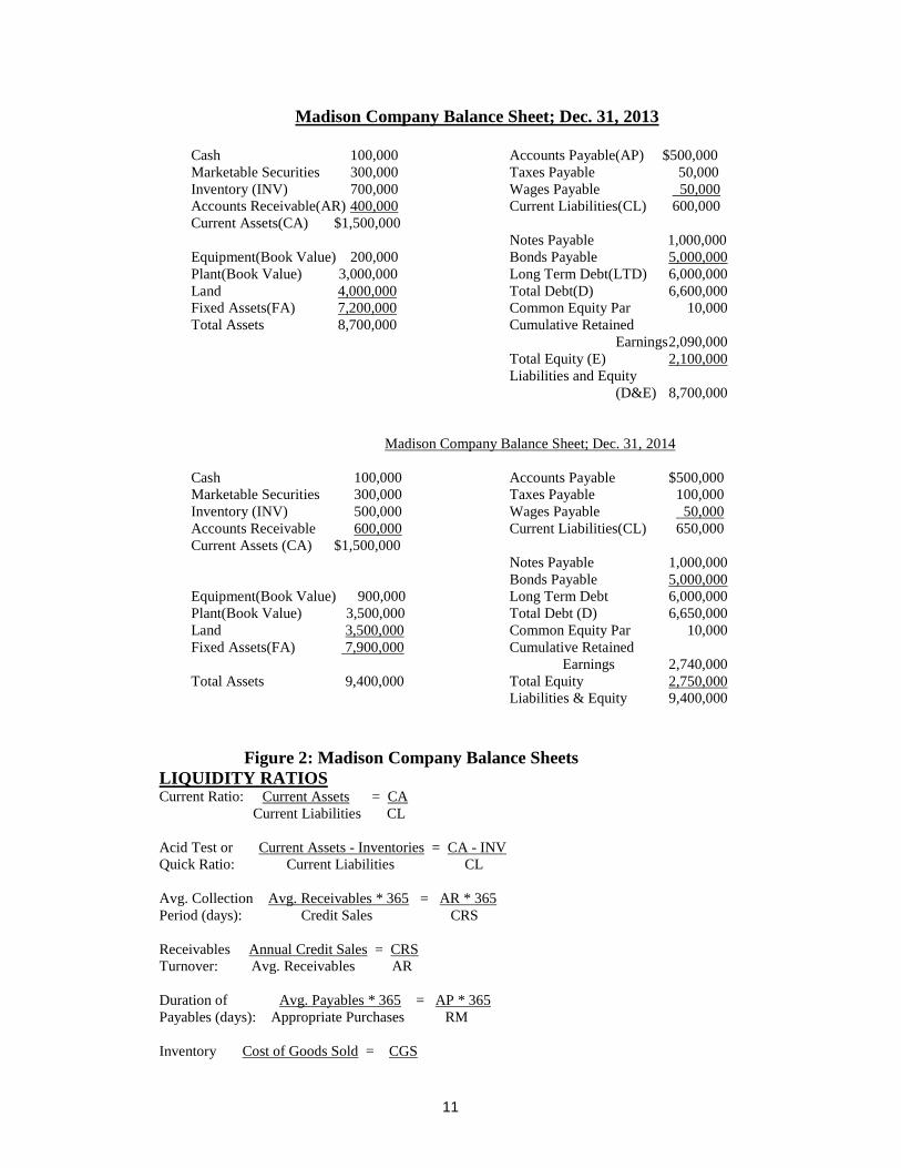
Madison Company Balance Sheet; Dec. 31, 2013

Cash 100,000 Accounts Payable(AP) $500,000

Marketable Securities 300,000 Taxes Payable 50,000

Inventory (INV) 700,000 Wages Payable 50,000

Accounts Receivable(AR) 400,000 Current Liabilities(CL) 600,000

Current Assets(CA) $1,500,000

Notes Payable 1,000,000

Equipment(Book Value) 200,000 Bonds Payable 5,000,000

Plant(Book Value) 3,000,000 Long Term Debt(LTD) 6,000,000

Land 4,000,000 Total Debt(D) 6,600,000

Fixed Assets(FA) 7,200,000 Common Equity Par 10,000

Total Assets 8,700,000 Cumulative Retained

Earnings 2,090,000

Total Equity (E) 2,100,000

Liabilities and Equity

(D&E) 8,700,000

Madison Company Balance Sheet; Dec. 31, 2014

Cash 100,000 Accounts Payable $500,000

Marketable Securities 300,000 Taxes Payable 100,000

Inventory (INV) 500,000 Wages Payable 50,000

Accounts Receivable 600,000 Current Liabilities(CL) 650,000

Current Assets (CA) $1,500,000

Notes Payable 1,000,000

Bonds Payable 5,000,000

Equipment(Book Value) 900,000 Long Term Debt 6,000,000

Plant(Book Value) 3,500,000 Total Debt (D) 6,650,000

Land 3,500,000 Common Equity Par 10,000

Fixed Assets(FA) 7,900,000 Cumulative Retained

Earnings 2,740,000

Total Assets 9,400,000 Total Equity 2,750,000

Liabilities & Equity 9,400,000

Figure 2: Madison Company Balance Sheets

LIQUIDITY RATIOS Current Ratio: Current Assets = CA

Current Liabilities CL

Acid Test or Current Assets - Inventories = CA - INV

Quick Ratio: Current Liabilities CL

Avg. Collection Avg. Receivables * 365 = AR * 365

Period (days): Credit Sales CRS

Receivables Annual Credit Sales = CRS

Turnover: Avg. Receivables AR

Duration of Avg. Payables * 365 = AP * 365

Payables (days): Appropriate Purchases RM

Inventory Cost of Goods Sold = CGS

Chapter 8

12

Turnover: Avg. Inventory Avg. Inv

Net Working Current Assets - Current Liab. = CA - CL

Capital to Total Assets TA

Total Assets:

PROFITABILITY RATIOS Return on Net Income After Tax = NIAT

Equity: Equity E

Return on Net Income After Tax + Int. = NIAT+Int.

Assets: Assets A

Gross Profit Sales - Cost of Goods Sold = S - CGS

Margin Ratio: Sales S

Net Profit Net Profit After Tax = NIAT


LEVERAGE RATIOS Financial Debt = D

Leverage: Debt + Equity D + E

Debt-Equity Debt = D

Ratio: Equity E

Times Interest Earnings Before Int. and Taxes = EBIT

Earned: Interest Payment Int.

ACTIVITY AND OTHER RATIOS

Sales Turnover: Total Sales = S

Total Assets A

Dividend Payout: Dividends = DIV

Net Income After Tax NIAT

Figure 3: LIST OF RATIOS

Ratio and Financial Statement Analysis

13

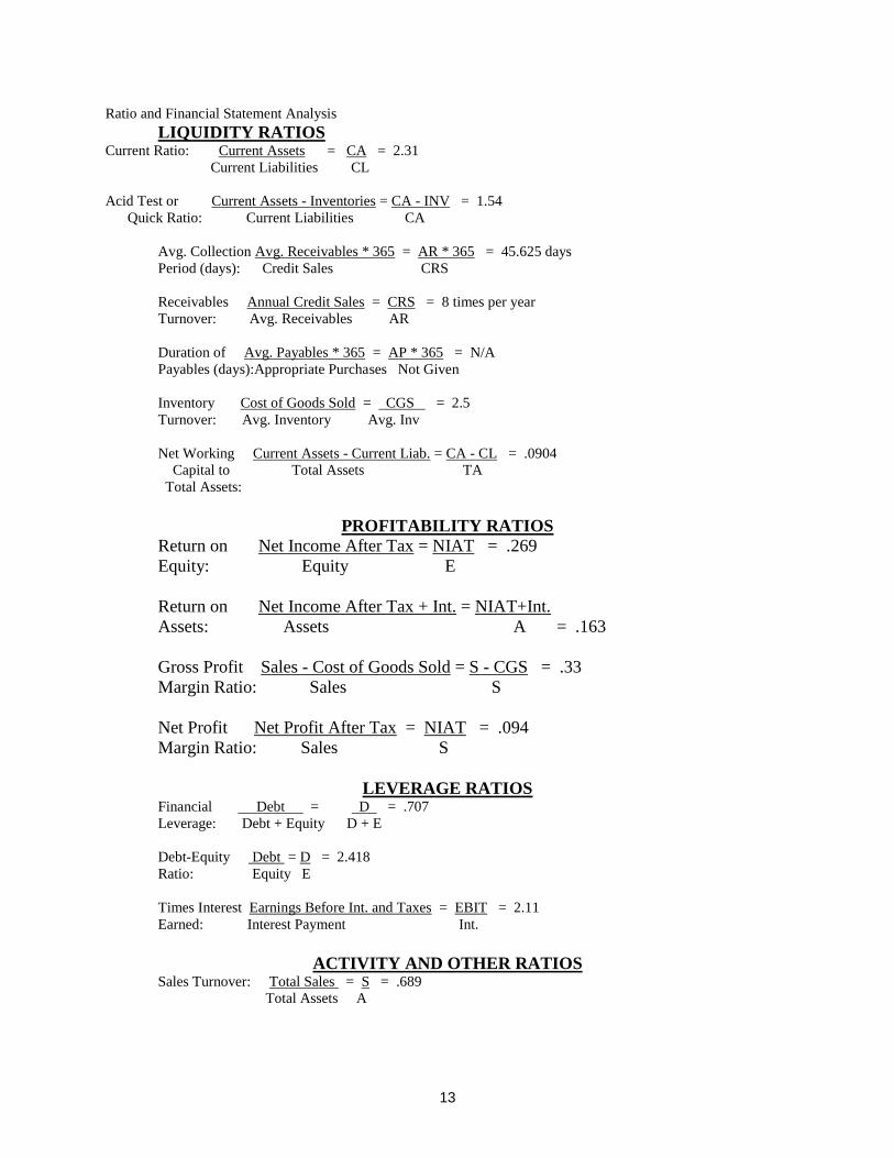
LIQUIDITY RATIOS Current Ratio: Current Assets = CA = 2.31

Current Liabilities CL

Acid Test or Current Assets - Inventories = CA - INV = 1.54

Quick Ratio: Current Liabilities CA

Avg. Collection Avg. Receivables * 365 = AR * 365 = 45.625 days

Period (days): Credit Sales CRS

Receivables Annual Credit Sales = CRS = 8 times per year

Turnover: Avg. Receivables AR

Duration of Avg. Payables * 365 = AP * 365 = N/A

Payables (days):Appropriate Purchases Not Given

Inventory Cost of Goods Sold = CGS = 2.5

Turnover: Avg. Inventory Avg. Inv

Net Working Current Assets - Current Liab. = CA - CL = .0904

Capital to Total Assets TA

Total Assets:

PROFITABILITY RATIOS

Return on Net Income After Tax = NIAT = .269

Equity: Equity E

Return on Net Income After Tax + Int. = NIAT+Int.

Assets: Assets A = .163

Gross Profit Sales - Cost of Goods Sold = S - CGS = .33


Net Profit Net Profit After Tax = NIAT = .094


LEVERAGE RATIOS Financial Debt = D = .707

Leverage: Debt + Equity D + E

Debt-Equity Debt = D = 2.418

Ratio: Equity E

Times Interest Earnings Before Int. and Taxes = EBIT = 2.11

Earned: Interest Payment Int.

ACTIVITY AND OTHER RATIOS Sales Turnover: Total Sales = S = .689

Total Assets A

Chapter 8

14

Dividend Payout: Dividends = DIV = .5

Net Income After Tax NIAT

Figure 4: FINANCIAL RATIOS FOR THE MADISON COMPANY

December 31,2014 or for Fiscal Year 2014


15

Ratio Disaggregation

Ratio analysis can be quite useful in locating firm difficulties. Common sense is

sometimes the best guide for their use; however, a number of useful analytical ratio techniques

have been devised. The multi-discriminant analysis described later in this chapter and

methodologies involving ratio disaggregation or decomposition such as DuPont analysis have

proven very useful tools for financial statement analysis and projections. Ratio disaggregation

decomposes a ratio into various component ratios facilitating analysis of the factors affecting the

original ratio in question. For example, consider the following disaggregation of Return on

Assets:

ROA = EBIT/Assets = Sales/Assets * GM/Sales * EBIT/GM

Thus, the firm’s return on assets can be disaggregated into the product of sales turnover, gross

margin and the inverse of the Degree of Operating Leverage. Hence, if the firm’s Return on

Assets were undesirably low, one or more of these ratios in the disaggregation would be low. In

fact, identification of the unexpected low ratio in the disaggregation might lead to explaining

why Return on Assets was so low. Suppose that the .1762 ROA for the Martin Company were

considered to be unacceptably low relative to the .2068 ROA ratio for the Madison Company.

The companies’ ROA ratios might be decomposed as follows:

.1762 = .4796 * .88 * .4176 (Martin)

.2068 = .6897 * .6667 * .45 (Madison)

One might observe that the Martin Company has a large sales to asset ratio relative to the

Madison Company. This might, at least in part, explain why its return on assets is lower.

Consider this second example, known as the DuPont identity, disaggregating return on

equity:

ROE = NIAT/Equity = NIAT/Sales * Sales/Assets * Assets/Equity

.221 = .1295 * .4796 * 3.564 (Martin)

.317 = .1108 * .6897 * 4.143 (Madison)

Balance sheet items were taken from the 2013 Balance sheets. This return on equity ratio (ROE)

is expressed as the product of one ratio from each of three ratio categories listed above:

Profitability * Activity * Leverage. Combining ratios from different categories demonstrates how

each category might impact shareholder returns. This Dupont identity reveals that Madison

Company seems to use its assets more efficiently, leading to a higher return on equity. Each of

these ratios could be further disaggregated. For example, the net margin ratio, NIAT/sales can be

decomposed as follows:

NIAT/Sales = NIAT/EBT * EBT/EBIT * EBIT/Sales

If a problem existed with a firm’s net profit margin, this decomposition and comparisons might

enable the analyst to better determine whether the source of the problem appears to be with tax

payments, interest payments or operations (gross margin.

Chapter 8

16

More generally, any ratio can be decomposed into a combination of other ratios. The

profitability ratios are most frequently decomposed. The decomposition method is to select (or

make up) ratios in such a manner such that when they are multiplied, all numerators cancel out

all denominators with the exception of one each. The remaining numerator and denominator

should be identical to those of the ratio being decomposed. Notice how the numerators and

denominators in the DuPont identity above cancel to leave NIAT and Equity as the remaining

numerator and denominator. The following factors might be called “profit drivers,” as they are

factors that will tend to increase returns on equity:

1. Net profit margin. Net profit margin is Net Income/Net Sales. It measures how

much of every sales dollar is profit. It can be increased by

a. Increasing sales volume.

b. Increasing sales price.

c. Decreasing expenses.

2. Asset turnover (efficiency). Asset turnover is Net Sales/Average Total Assets.

It measures how many sales dollars the company generates with each dollar of

assets. It can be increased by

a. Increasing sales volume.

b. Disposing of (decreasing) less productive assets.

3. Financial leverage. Financial leverage is Average Total Assets/Average

Stockholders’ Equity. It measures how many dollars of assets are employed for

each dollar of stockholder investment. It can be increased by

a. Increased borrowing.

b. Repurchasing (decreasing) outstanding stock.


17

D. Misreading and Misleading Financial Statements

In an ideal world, financial statements would be intended to give clear and accurate

portrayals of economic value and information needed to make economic decisions.

Unfortunately, it is not possible to follow through on this ideal, and financial statements are, in

reality, subject to a myriad of complicated accounting rules and regulations, differences in

interpretation and application, subject to omissions and, in the worst cases, deception. An

equities analyst would certainly benefit from training in accounting, at a minimum, introductory

and intermediate accounting along with financial statement analysis. There are a number of

excellent books that deal with the subject, including those that are used to prepare candidates for

the CFA certification.1

First, managers are under intense pressure to meet revenue and earnings targets. For

example, Skinner and Sloan [2002] find that when firms announce quarterly earnings beating

consensus analyst forecasts, stock prices show abnormal price increases averaging 5.5%.

Negative earnings surprises result in abnormal price declines averaging -5.04%. Most

professional analysts are aware that they must view income statements and earnings reports with

at least some skepticism. For example, consider some of the abuses that occur with revenue

recognition. To realize sales projections or revenue increases, a company may slash prices, relax

credit standards and cut deals at the end of the quarter to off-load products to dealers when there

is no underlying retail demand. These deliveries of goods still count as sales. Sometimes firms

will ship their products on or close to Dec. 31 in order to record the sale for the year just ending.

However, the company receiving the shipment after the new-year may record the purchase

expense for the new-year. For example, under the leadership of “Chainsaw” Al Dunlap,

appliance maker Sunbeam Corp. was forced to restate financial results for 1996 and 1997 after

the firm was accused of using this type of phony accounting to boost profits. The company later

filed for bankruptcy. At the root of this fraud was Sunbeam’s having made side agreements with

customers to accept product deliveries prematurely, where products were shipped to warehouses

with rights to refuse the shipment. IBM (with its 2001 $340 million sale of optical transceiver

business to JDS Uniphase on the final day of the quarter) and Xerox were among the many

companies to have been accused of such practices.

Many analysts and investors are impressed with companies that can demonstrate a long

history of uninterrupted earnings growth. Myers, Myers and Skinner (2007) found that firms that

experienced the same average rate and growth rate of returns over 20 quarters, those firms whose

earnings growth rates were consistently positive sold at a 6% premium over those firms that had

experienced at least one quarter where earnings did not grow. In their study concerning earnings

manipulation, they calculated that over the 42-year period of their study, no more than 18-46

companies should have experienced more than 20 consecutive quarters of uninterrupted earnings

growth. This figure, based on simulations, assumed that no companies manipulated their

earnings levels. However, in their study, the actual number of firms with more than 20 quarters

of uninterrupted earnings growth was 587, suggesting that companies do manage their earnings

to maintain consistent earnings growth.

Consider a survey by Graham, Harvey and Rajgopal [2005] of 401 corporate CFOs

asking the following question: “Near the end of the quarter, it looks like your company might

come in below the desired earnings target. Within what is permitted by GAAP, which of the

1 For example, see White, Gerald I., Ashwinpaul C. Sondhi and Dov Fried (2002). The Analysis and Use of

Financial Statements, 3rd Ed. New York: Wiley Publishers.

Chapter 8

18

following choices might your company make?” Their survey results indicated that 80% of these

CFOs companies would be willing to delay discretionary spending such as R&D, advertising and

maintenance, and over 55% would knowingly sacrifice small value increases by delaying the

project starts. Almost 40% would speed revenue generation. Glater.[2005] reported that a record

number (253) of public companies restated their annual audited financial statements in 2004 and

161 companies restated their quarterly statements.2

The analyst should take care to examine sudden changes in sales levels, performing

comparisons with peer firms and with prior years’ data. Common size accounting statements

(where sales are standardized at 100 and other income statement items are expressed as fractions

of 100) are often helpful for such comparisons. Checks for relaxation in credit standards (e.g.,

significant growth in Accounts Receivable relative to sales) should be performed when suspicion

arises.

Similar sorts of games have been played with operating expenses. The GAAP guideline

known as the matching principle requires companies to match expenses with corresponding

reported revenues. Companies have ignored this requirement, deferring current expenses or by

capitalizing normal operating expenses as assets. This technique can temporarily boost current

earnings. Enron, WorldCom and AOL (both by capitalizing expenses) and Cendant (whose $100

million restatement cost shareholders $15 billion in a single day) are among the firms that have

been accused of these abuses.

Accounting restatements may create even more significant problems for the firm’s

investors. The United States General Accounting Office (GAO) reported that the number of

restatements grew by 300% from 1997 through 2004. Numerous studies have shown that

financial restatements adversely impact firm value (e.g., Dechow, Sloan and Sweeney [1996]).

For example, Kinney and McDaniel (1989) characterized firms filing restatements of quarterly

earnings reports, finding that these firms were smaller, less profitable, exhibited slower growth;

had greater leverage and received more qualified audit opinions than their industry counterparts.

Financial restatements are costly to the firm. They lead to unfavorable publicity, can trigger SEC

and other formal investigations, impair the credibility of firm executives and can lead to their

replacement. Financial restatements imply impaired transparency and reduce the reliability of the

accounting statements of the firm. In addition, restatements can be expected to alter investors’

perceptions of current and future performance and value.

Relatively recent bankruptcies related to accounting fraud include Enron, McKesson

HBOC, ConAgra, Sybase, S3, Fine Host, Versatility, Physicians’ Computer, Medaphis,

Parmalat, Centennial Technology, WorldCom, Norland Medical, Premier Laser, Altris Software,

Micro Warehouse, Transcrypt, Sunbeam, Paracelsus, DonnKenny, RasterGraphics, Covad and

TriTeal. However, much of the difficulty in interpreting financial statements is not related to

fraud; it is simply difficult to use accounting statements to accurately reflect economic values.

But, there may not be any better alternatives.

Balance sheets can also be affected by deception and questions of interpretation.

Contingent liabilities are always a source of difficulty, especially when potential payoffs and

their probabilities simply cannot be known. Footnotes should be carefully scrutinized. Special

purpose entities, subsidiaries, pyramid structures and cross ownership should always be carefully

examined.

2 See Jensen [2005] for a discussion of these and related results.


19

Example: Cross-ownership and Share Value Inflation

Cross ownership exists when firms own shares of each others’ stock. Firms often

purchase shares for investment purposes and may own each other’s shares to forge strategic

alliances ad for other purposes. Cross ownership of shares is a very common phenomenon in

many parts of the world such as in Japan with the keiretsu, Korea with the chaebol and in Europe

with privately held companies. It has also been used to create deceptions of several types. For

example, Enron Corporation created a number of “special purpose entities” that it used to place

the parent firm’s debt and equity securities. Such placements contributed to the fall of Enron.

Parmalat, in a case that we will discuss later, used off shore subsidiaries to hide non-performing

assets and certain liabilities. In the late 1990s (and even today), many companies in the

telecommunications and cable industries hold shares of each other’s stock. Such cross holdings

inflated the book values of equity of these firms since the equity held by each company increased

the book value of the equity held by other companies that hold its shares. This will be illustrated

below. Pyramid schemes employing cross-ownership have long been used to create the

perception of wealth that simply does not exist.

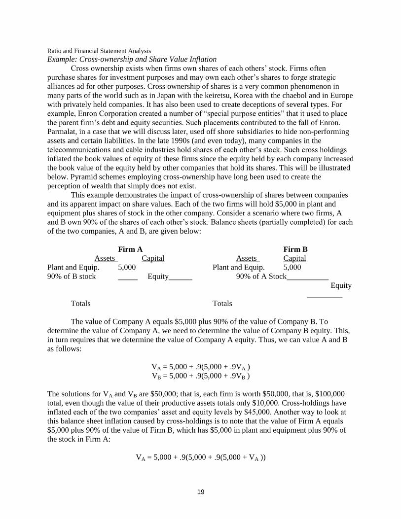
This example demonstrates the impact of cross-ownership of shares between companies

and its apparent impact on share values. Each of the two firms will hold $5,000 in plant and

equipment plus shares of stock in the other company. Consider a scenario where two firms, A

and B own 90% of the shares of each other’s stock. Balance sheets (partially completed) for each

of the two companies, A and B, are given below:

Firm A Firm B Assets Capital Assets Capital

Plant and Equip. 5,000 Plant and Equip. 5,000

90% of B stock Equity 90% of A Stock

Equity

_________

Totals Totals

The value of Company A equals $5,000 plus 90% of the value of Company B. To

determine the value of Company A, we need to determine the value of Company B equity. This,

in turn requires that we determine the value of Company A equity. Thus, we can value A and B

as follows:

VA = 5,000 + .9(5,000 + .9VA )

VB = 5,000 + .9(5,000 + .9VB )

The solutions for VA and VB are $50,000; that is, each firm is worth $50,000, that is, $100,000

total, even though the value of their productive assets totals only $10,000. Cross-holdings have

inflated each of the two companies’ asset and equity levels by $45,000. Another way to look at

this balance sheet inflation caused by cross-holdings is to note that the value of Firm A equals

$5,000 plus 90% of the value of Firm B, which has $5,000 in plant and equipment plus 90% of

the stock in Firm A:

VA = 5,000 + .9(5,000 + .9(5,000 + VA ))

Chapter 8

20

which, since Firm A value equals $5000 plus 90% of the value of Firm B:

VA = 5,000 + .9(5,000 + .9(5,000 + (5,000 + VB )))

or, more generally,

VA = 5,000 (.90

+ .91

+ .92

+ . . . + .9)

We can simplify this expression with a geometric expansion to obtain:3

VA = 5,000/.1 = 50,000

Regardless, cross ownership has inflated the value of each company from $5,000 to $5,000/(1-.9)

= $45,000. Cross ownership, in and of itself, is not necessarily fraudulent or abusive, but it is a

practice that analysts need to be aware of when examining accounting statements.

3 Multiply both sides by .9VA to obtain .9VA = 5,000 (.9

1 + .9

2 + . . . + .9

+1) and then subtract this equation

from VA to obtain VA - .9VA = 5,000 (.90

- .9+1

). Simplify further to obtain VA(1-.9) = 5,000(1), which leads to

VA = 5,000/.1 = 50,000.


21

E. Comparables-Based Valuation

While we have spent much time on growth models and forecasting dividends, earnings

and free cash flows, market-based ratios from comparable firms are used more frequently by

equity analysts to derive firm values. The results of such comparisons seem less sensitive to

estimation errors and require less forecasting ability. Using the Relative Valuation

(Comparables) Approaches involves comparing the target firm to a group of other firms with

similar operating circumstances. In some instances, there will be obvious firms to serve as

comparisons. Many analysts rely on Standard Industrial Classification (SIC) or North American

Industry Classification System (NAICS) codes to identify a target firm’s peer group. Several

institutions such as Dun and Bradstreet provide data useful for comparisons of ratios. For

example, Dun and Bradstreet provides "average" ratio levels for firms in a number of different

industries.

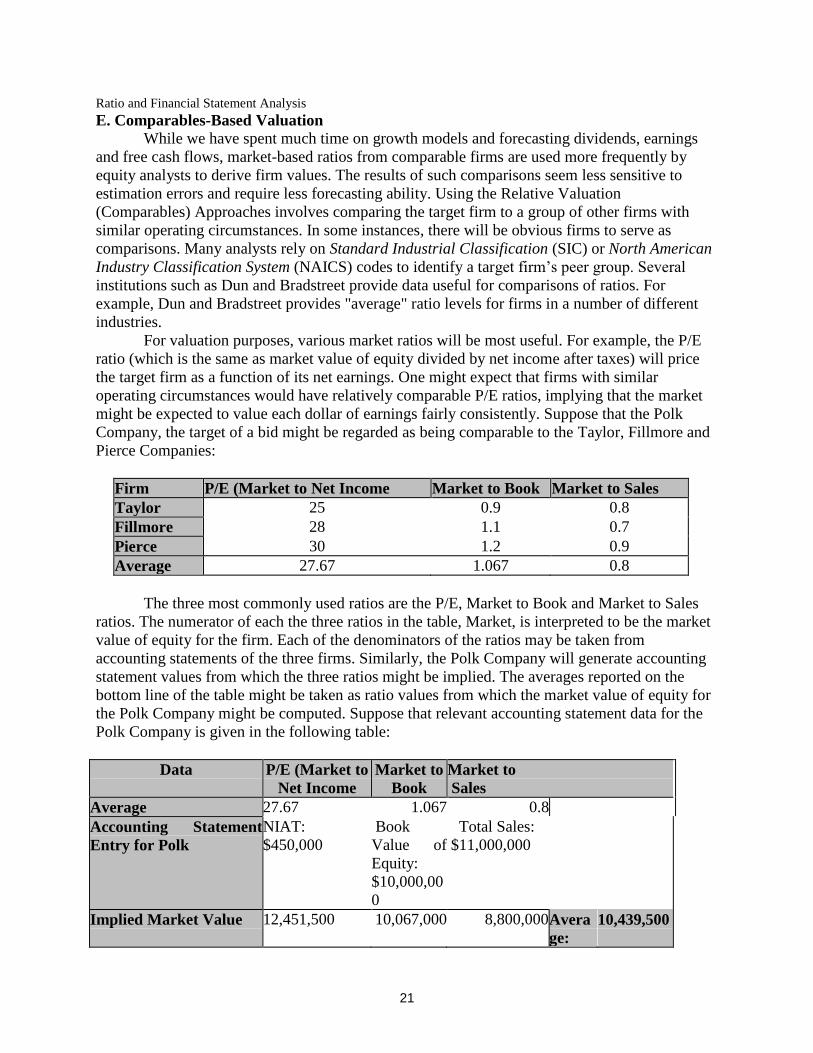
For valuation purposes, various market ratios will be most useful. For example, the P/E

ratio (which is the same as market value of equity divided by net income after taxes) will price

the target firm as a function of its net earnings. One might expect that firms with similar

operating circumstances would have relatively comparable P/E ratios, implying that the market

might be expected to value each dollar of earnings fairly consistently. Suppose that the Polk

Company, the target of a bid might be regarded as being comparable to the Taylor, Fillmore and

Pierce Companies:

Firm P/E (Market to Net Income Market to Book Market to Sales

Taylor 25 0.9 0.8

Fillmore 28 1.1 0.7

Pierce 30 1.2 0.9

Average 27.67 1.067 0.8

The three most commonly used ratios are the P/E, Market to Book and Market to Sales

ratios. The numerator of each the three ratios in the table, Market, is interpreted to be the market

value of equity for the firm. Each of the denominators of the ratios may be taken from

accounting statements of the three firms. Similarly, the Polk Company will generate accounting

statement values from which the three ratios might be implied. The averages reported on the

bottom line of the table might be taken as ratio values from which the market value of equity for

the Polk Company might be computed. Suppose that relevant accounting statement data for the

Polk Company is given in the following table:

Data P/E (Market to

Net Income

Market to

Book

Market to

Sales

Average 27.67 1.067 0.8

Accounting Statement

Entry for Polk

NIAT:

$450,000

Book

Value of

Equity:

$10,000,00

0

Total Sales:

$11,000,000

Implied Market Value 12,451,500 10,067,000 8,800,000 Avera

ge:

10,439,500

Chapter 8

22

With data from each of the three peer firms weighted identically, and values taken from

Polk Company accounting statements, we find that potential values of the Polk Company are

$12,451,500, $10,067,000 and $8,800,000. If we were to weight these values equally, we would

value the Polk Company at $10,439,500. A share price for Polk can be obtained by dividing

$10,439,500 by the number of outstanding shares.

Performance: DCF versus Comparables

We have discussed DCF and Comparables analysis in this chapter. Which works better?

First, it is clear that most analysts make more extensive use of price multiples than DCF.

However, as we will discuss later, in their study of 51 highly leveraged transactions, Kaplan and

Ruback [1995] found that DCF analysis provided better estimates of value than price-based

multiples, though the price-based multiples did add useful information to the valuation process.

Some analysts have noted that the comparables approach does not provide a proper accounting

for risk differences among companies and does not allow for differences in growth and super-

growth opportunities. Such market-based comparisons may be vulnerable to short-term price

fluctuations or temporary accounting statement changes.

Other research (e.g., Lie and Lie [2002]) has suggested that price multiples may be more

useful for IPOs and other valuations where future cash flows are particularly difficult to estimate.

However, highly comparable companies must still be made available for comparison. In

addition, negative earnings, as is so common for IPO companies and their peers, can create bias

or render the more simple comparisons meaningless.


23

References

Dechow, P., R. Sloan, and A. Sweeney, 1996, Causes and consequences of earnings

manipulation, an analysis of firms subject to enforcement actions by the SEC, Contemporary

Accounting Research 13, 1–36.

Glater. J.D. (2005): “Restatements, and Lawsuits, are on the Rise.” New York Times, January 20.

Graham. J.R., C.R. Harvey, and S. Rajgopal (2005): “The Economic Implications of Corporate

Financial Reporting,” Journal of Accounting and Economics.

Jensen, Michael (2005): “Agency Costs of Overvalued Equity,” Financial Management, Spring,

pp. 5-19.

Kaplan, Steven N. and Richard S. Ruback (1995). “The Valuation of Cash Flow Forecasts: An

Empirical Analysis,” Journal of Finance 50, no. 4 (September), pp. 1059-1093.

Kinney, W. R. Jr., and L. S. McDaniel, 1989, Characteristics of firms correcting previously

reported quarterly earnings, Journal of Accounting and Economics 11, 71–93.

Lie, Eric and Heidi Lie (2002): “Multiples Used to Estimate Corporate Value,” Financial

Analysts Journal March/April pp. 1-11.

Myers, James N., Linda A. Myers and Douglas J. Skinner (2007). Earnings Momentum and

Earnings Management,” Journal of Accounting, Auditing and Finance, Spring.

Skinner. D.J. and R.G Sloan (2002): “Earnings Surprises. Growth Expectations, and Stock

Returns or Don't Let an Earnings Torpedo Sink Your Portfolio,” Review of Accounting Studies 1.

289-312.

White, Gerald I., Ashwinpaul C. Sondhi and Dov Fried (2002). The Analysis and Use of

Financial Statements, 3rd Ed. New York: Wiley Publishers.

Weston, J. Fred, Kwang S. Chung and Susan E. Hoag (1990): Mergers, Restructuring and

Corporate Control, Englewood Cliffs, New Jersey: Prentice-Hall.

Chapter 8

24

Exercises

7.1. The following are accounting statements for the Jeffries Sporting Goods Company:

Income Statement, 2014 Balance Sheet, Dec.31,2013

Rev......$800,000 ASSETS CAPITAL

CGS.......100,000 Cash.........$25,000 Tax Payable.$25,000

FC........300,000 Mkt. Secs.....75,000 A.P..........75,000

EBIT......400,000 Accts. Rec...350,000 C.L.........100,000

INT.......100,000 Inv..........250,000 Notes Pay...300,000

EBT.......300,000 C.A..........700,000 Bonds Pay...600,000

Taxes.....100,000 Plant&Equip..900,000 L.T.D.......900,000

NIAT......200,000 Fixed Assets.900,000 Debt......1,000,000

Div....... 50,000 Equity......600,000

RE........150,000 Assets.....1,600,000 Capital...1,600,000

The following are accounting statements for the Tunney Sporting Goods Company: Income Statement, 2014 Balance Sheet, Dec.31,2013

Rev......$600,000 ASSETS CAPITAL

CGS........60,000 Cash........$100,000 Tax Payable.$75,000

FC........300,000 Mkt. Secs.....30,000 A.P.........225,000

EBIT......240,000 Accts. Rec...170,000 C.L.........300,000

INT.......150,000 Inv..........200,000 Notes Pay...200,000

EBT........90.000 C.A..........500,000 Bonds Pay...400,000

Taxes......30,000 Plant&Equip..950,000 L.T.D.......600,000

NIAT.......60,000 Fixed Assets.950,000 Debt........900,000

Div........50,000 Equity......550,000

RE.........10,000 Assets.....1,450,000 Capital...1,450,000

a. Compute the following ratios for each of the two sporting

goods companies:

i. Current Ratio

ii. Acid Test Ratio

iii. Net Working Capital to Total Assets

iv. Return on Equity

v. Return on Assets

vi. Gross Profit Margin

vii. Net Profit Margin

viii.Financial Leverage Ratio

ix. Debt-Equity Ratio

x. Times Interest Earned Ratio

xi. Dividend Payout

b. Which of the two companies seems to operate more efficiently?

c. How did you measure efficiency?

d. Why is this company capable of operating more efficiently?

e. What advice would you give to managers of the two companies on the basis of the accounting

statement information and ratios?

f. Which company would you prefer to lend money to? Why?


25

g. In your opinion, what are the probabilities associated with either company defaulting on its

debt

obligations?

h. What are your estimates for NIAT for both companies in 2015, given that each expects a 2015

sales level of $500,000?

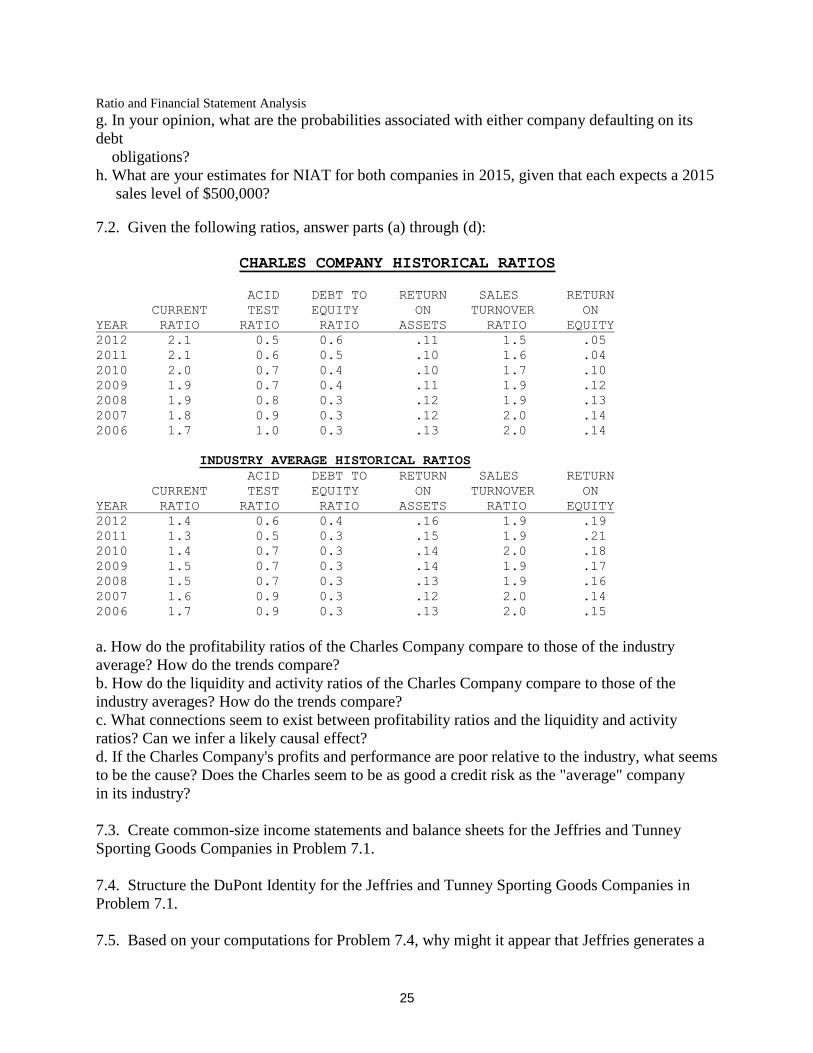
7.2. Given the following ratios, answer parts (a) through (d):

CHARLES COMPANY HISTORICAL RATIOS

ACID DEBT TO RETURN SALES RETURN

CURRENT TEST EQUITY ON TURNOVER ON

YEAR RATIO RATIO RATIO ASSETS RATIO EQUITY

2012 2.1 0.5 0.6 .11 1.5 .05

2011 2.1 0.6 0.5 .10 1.6 .04

2010 2.0 0.7 0.4 .10 1.7 .10

2009 1.9 0.7 0.4 .11 1.9 .12

2008 1.9 0.8 0.3 .12 1.9 .13

2007 1.8 0.9 0.3 .12 2.0 .14

2006 1.7 1.0 0.3 .13 2.0 .14

INDUSTRY AVERAGE HISTORICAL RATIOS

ACID DEBT TO RETURN SALES RETURN

CURRENT TEST EQUITY ON TURNOVER ON

YEAR RATIO RATIO RATIO ASSETS RATIO EQUITY

2012 1.4 0.6 0.4 .16 1.9 .19

2011 1.3 0.5 0.3 .15 1.9 .21

2010 1.4 0.7 0.3 .14 2.0 .18

2009 1.5 0.7 0.3 .14 1.9 .17

2008 1.5 0.7 0.3 .13 1.9 .16

2007 1.6 0.9 0.3 .12 2.0 .14

2006 1.7 0.9 0.3 .13 2.0 .15

a. How do the profitability ratios of the Charles Company compare to those of the industry

average? How do the trends compare?

b. How do the liquidity and activity ratios of the Charles Company compare to those of the

industry averages? How do the trends compare?

c. What connections seem to exist between profitability ratios and the liquidity and activity

ratios? Can we infer a likely causal effect?

d. If the Charles Company's profits and performance are poor relative to the industry, what seems

to be the cause? Does the Charles seem to be as good a credit risk as the "average" company

in its industry?

7.3. Create common-size income statements and balance sheets for the Jeffries and Tunney

Sporting Goods Companies in Problem 7.1.

7.4. Structure the DuPont Identity for the Jeffries and Tunney Sporting Goods Companies in

Problem 7.1.

7.5. Based on your computations for Problem 7.4, why might it appear that Jeffries generates a

Chapter 8

26

much higher return to shareholders?

chapter 7 ratio and financial statement · pdf file1 chapter 7 ratio and financial statement...

Documents