Ch

ap

ter 7

PRODUCTION

McGraw-Hill/Irwin Copyright © 2011 by The McGraw-Hill Companies, Inc. All rights reserved.

Ch

ap

ter 7

9-3

Chapter Outline

• The Production Function• Production In The Short Run• Production In The Long Run• Returns To Scale

9-4

The Production Function

• Production function: the relationship that describes how inputs like capital and labour are transformed into output.

• Mathematically,

Q = F (K, L)K = CapitalL = Labour

9-5

Figgure 7.1: A Production Worker

9-6

Figure 7.2: The Production Function InputsLand, labour, capital, and so forth

Outputs(cars, polio vaccine,home-cooked meals,TV broadcasts, and so forth)

9-7

The Production Function

• Long run: the shortest period of time required to alter the amounts of all inputs used in a production process.

• Short run: the longest period of time during which at least one of the inputs used in a production process cannot be varied.

• Variable input: an input that can be varied in the short run.

• Fixed input: an input that cannot vary in the short run.

9-8

Short-run Production Funtion

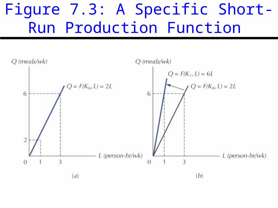
• Three properties:1.It passes through the origin.2.Initially the addition of variable inputs augments

output at an increasing rate.3.Beyond some point additional units of the variable

input give rise to smaller and smaller increments in output.

9-9

Figure 7.3: A Specific Short-Run Production Function

9-10

Figure 7.4: Another Short-Run Production Function

9-11

Short-run Production Function

• Law of diminishing returns: if other inputs are fixed, the increase in output (marginal product) from an increase in the variable input must eventually decline.

9-12

Figure 7.5: The Effect of Technological Progress in Food Production

Q2010

Q1810

L2010L18100

9-13

Short-run Production Function

• Total product curve: a curve showing the amount of output as a function of the amount of variable input.

• Marginal product: change in total product due to a 1-unit change in the variable input.

• Average product: total output divided by the quantity of the variable input.

9-14

Figure 7.6: The Marginal Productof a Variable Input

0

9-15

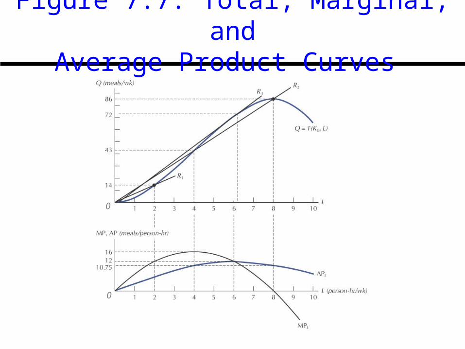
Figure 7.7: Total, Marginal, andAverage Product Curves

0

0

9-16

Relationship between Total, Marginal and Average Product Curves

• When the marginal product curve lies above the average product curve, the average product curve must be rising.

• When the marginal product curve lies below the average product curve, the average product curve must be falling.

• The two curves intersect at the maximum value of the average product curve.

9-17

The Practical Significance Of The Average -Marginal Distinction

• Suppose you own a fishing fleet consisting of a given number of boats, and can send your boats in whatever numbers you wish to either of two ends of an extremely wide lake, east or west. Under your current allocation of boats, the ones fishing at the east end return daily with 100 kilograms of fish each, while those in the west return daily with 120 kilograms each. The fish populations at each end of the lake are completely independent, and your current yields can be sustained indefinitely.

• Should you alter your current allocation of boats?

9-18

The Practical Significance Of The Average -Marginal Distinction

• The general rule for allocating an input efficiently in such cases is to allocate the next unit of the input to the production activity where its marginal product is the highest.

9-19

Figure 7.8: Effectiveness vs. Use: Lobs and Passing Shots

0

9-20

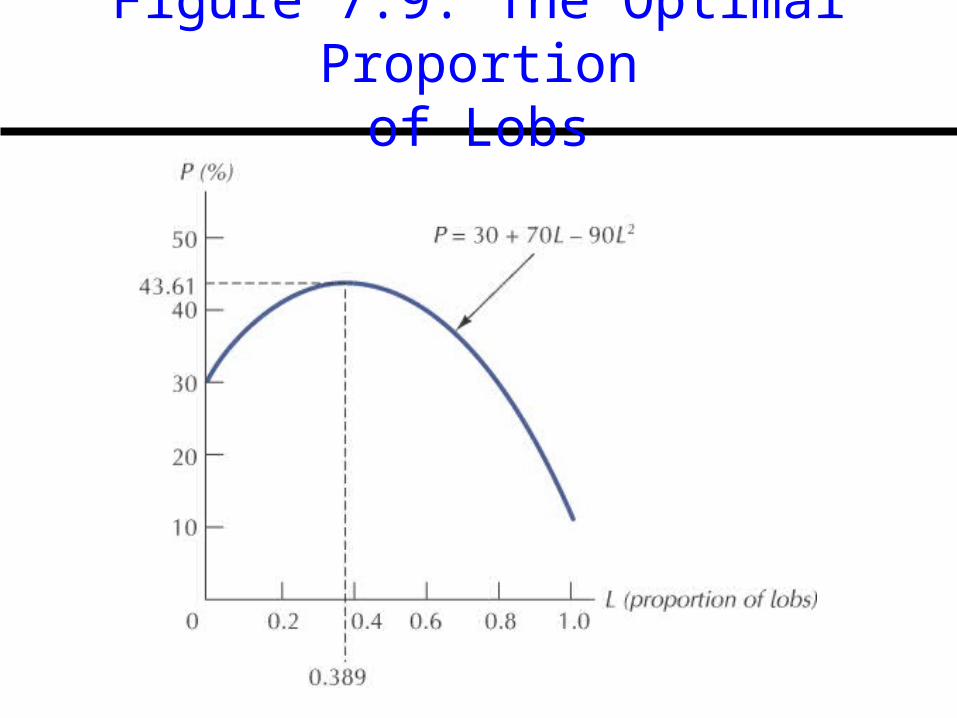
Figure 7.9: The Optimal Proportionof Lobs

9-21

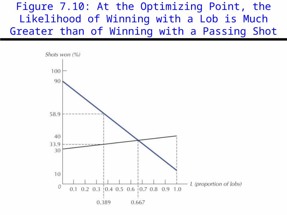
Figure 7.10: At the Optimizing Point, the Likelihood of Winning with a Lob is Much Greater than of Winning with a Passing Shot

0

9-22

Production In The Long Run

• Isoquant: the set of all input combinations that yield a given level of output.

• Marginal rate of technical substitution (MRTS): the rate at which one input can be exchanged for another without altering the total level of output.

9-23

Figure 7.11: Part of an Isoquant Map for the Production Function Q = 2KL

Labour (L)0

9-24

Figure 7.12: Isoquant Map for the Cobb-DouglasProduction Function Q = K½L½

9-25

Figure 7.13: Isoquant Map for the Leontief Production Function Q = min (2K,3L)

9-26

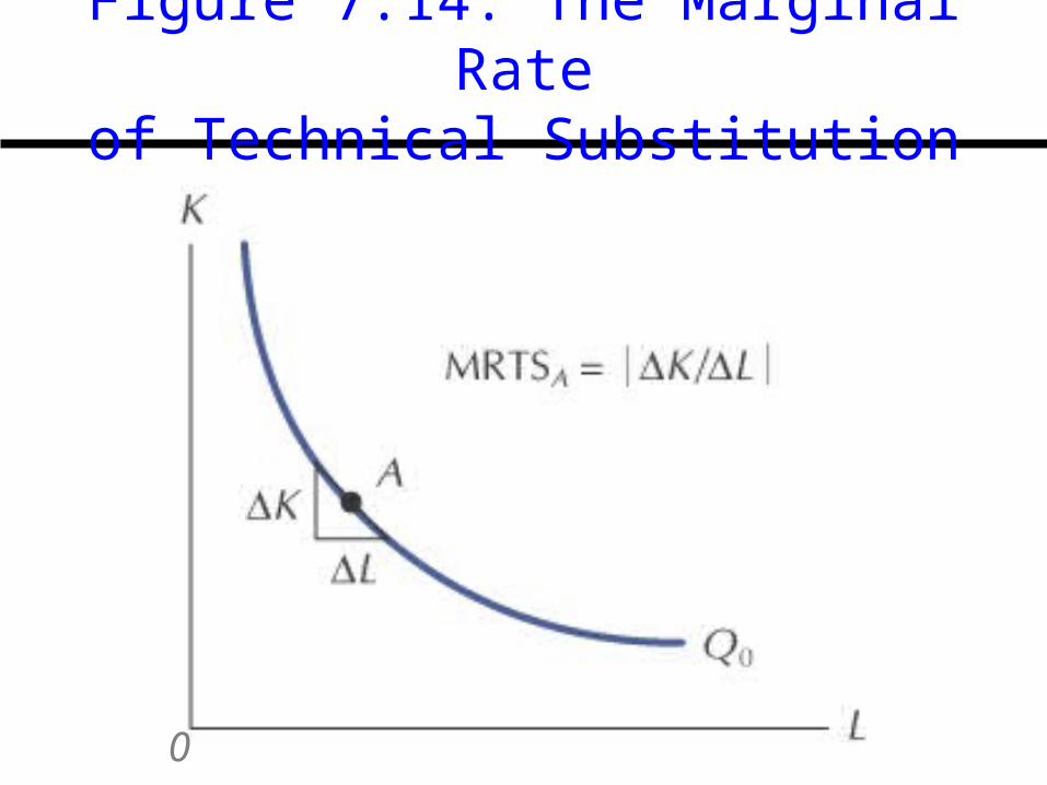
Figure 7.14: The Marginal Rateof Technical Substitution

0

9-27

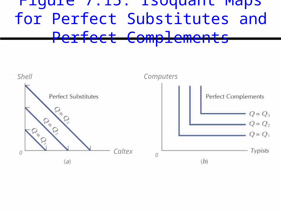
Figure 7.15: Isoquant Maps for Perfect Substitutes and Perfect Complements

Shell

Caltex

Computers

0 0

9-28

Returns To Scale

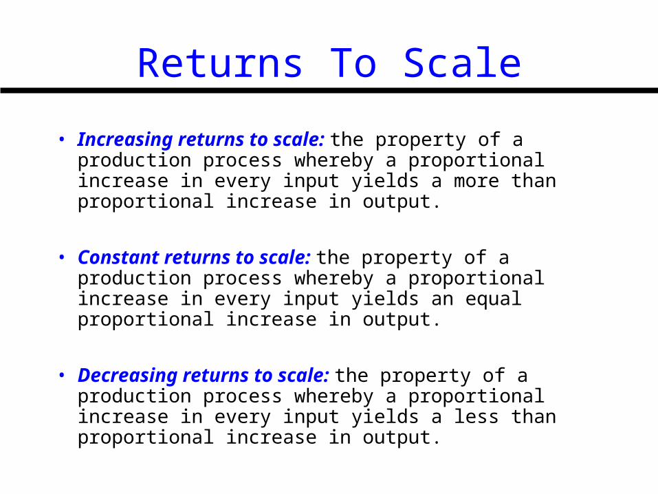
• Increasing returns to scale: the property of a production process whereby a proportional increase in every input yields a more than proportional increase in output.

• Constant returns to scale: the property of a production process whereby a proportional increase in every input yields an equal proportional increase in output.

• Decreasing returns to scale: the property of a production process whereby a proportional increase in every input yields a less than proportional increase in output.

9-29

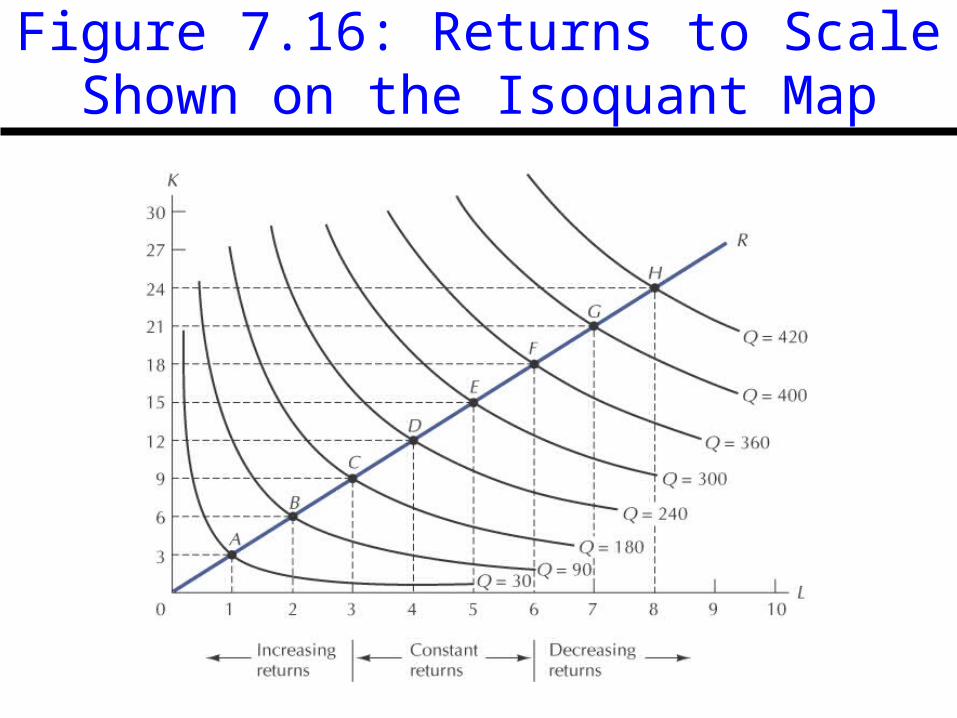
Figure 7.16: Returns to Scale Shown on the Isoquant Map