126

CHAPTER 7

POLARIZATION-SENSITIVE MULTIPATH PROPAGATION MODELING

7.1 Introduction

A variety of propagation models have been reported in the literature that

approximate characteristics of a radio channel, including path loss, shadowing, and

multipath effects. These models provide some insight into the effects of different channel

characteristics on wireless communication systems. Models can be used for preliminary

evaluation of system alternatives before investing in prototype hardware.

Current propagation models do not consider the polarization of transmitted signal,

depolarization introduced by the channel, or polarized multipath. Propagation models

that include polarization effects will be useful for evaluating the performance of

polarization-sensitive adaptive arrays and diversity reception techniques. While

polarization-sensitive adaptive arrays have been proposed as described in Chapter 5, their

performance has not been evaluated in multipath channels. In this chapter, existing

multipath propagation models are extended to include the effects of antenna pattern,

antenna orientation, and wave polarization.

7.2 Existing Multipath Propagation Models

Many multipath propagation models have been developed for evaluating antenna

diversity and adaptive array systems. Several of these models are summarized in [7.1].

These models typically assume there are a number of objects that cause scattering or

specular reflections (for brevity both of these will be referred to as “scatterers”) in the

vicinity of the transmitter and/or receiver. The signal at the receiver consists of signals

reflected or scattered from objects, and possibly also a line-of-sight component. These

models generate several multipath components, each having distinct amplitude, phase,

and angle of arrival at each receiving antenna. The models yield a vector containing the

resultant signal at each antenna due to all the multipath components. Because of this,

these models are sometimes called vector channel models.

Site-specific propagation prediction approaches such as ray tracing and finite-

difference time domain (FDTD) are deterministic and exploit knowledge of physical

objects in the propagation environment and their properties. These models can provide

127

good agreement with measured results [7.2], but detailed information on the size, shape,

and location of objects in the channel is required. In addition, extensive measurements

are required to optimize such models for a specific location.

In contrast, more general models like those described in this section address

channels with specific characteristics (i.e. multipath delay and angle spread) but do not

attempt to represent a specific channel exactly. The models discussed here include free-

space path loss and are useful for simulating multipath effects but do not attempt to

simulate the effects of shadowing. These models can be deterministic, with scatterers

placed in specific locations, as in Lee’s model, or stochastic like Liberti’s and Petrus’

models, where scatterers are distributed randomly. Deterministic simulations can be

performed using a specific sample of scatterers from the Petrus or Liberti models, but the

scatterer locations are not chosen to simulate a particular physical channel as they are in

site-specific models.

Propagation conditions in a wireless communication system vary depending on

the position of the mobile or hand-held unit. The line-of-sight path is obstructed in some

cases but not others. The channel models described in this chapter represent a “worst

case” where several multipath components have similar power levels. In this scenario

very deep fades occur. These models require much less information and computation

than site-specific models such as ray tracing and FDTD, and are useful for assessing the

performance of a system in a range of channel conditions. Three general vector channel

models are discussed below.

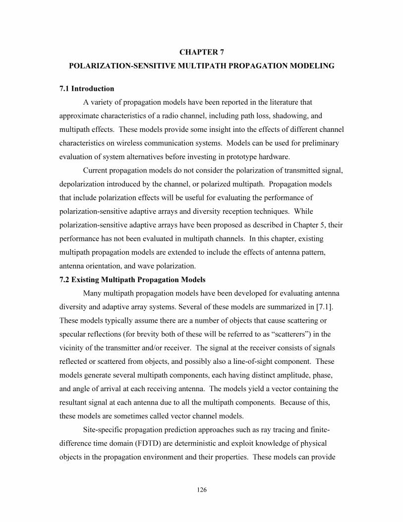
7.2.1 Ring of scatterers model (Lee)

Lee’s model [7.3] assumes that the base station antenna is located above the

terrain and buildings, as in a macrocell system, so that reflections occur near the mobile

and not near the base station. In this model, scatterers are evenly spaced on a circle about

the mobile as shown in Fig. 7-1. The radius of the ring of scatterers is 30-60 m or about

100-200 wavelengths at 850 MHz. The contribution of the reflected ray from each

scatterer at the receiver is calculated. Several variations on this model are discussed in

[7.1].

128

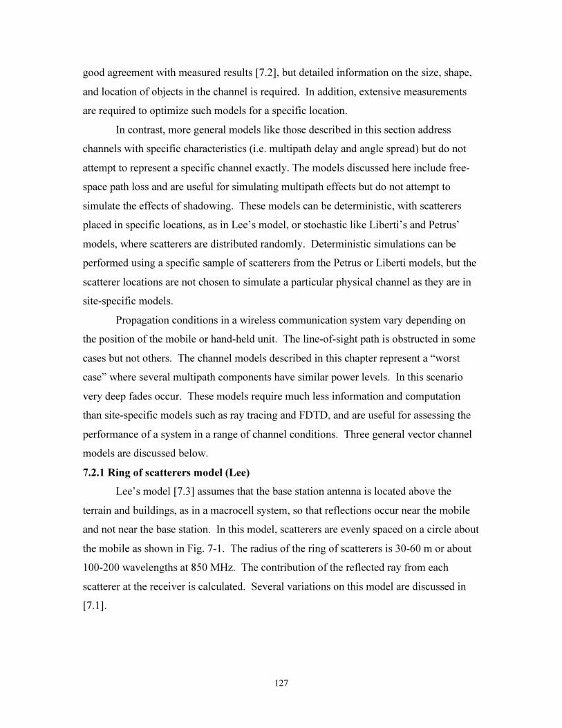
Figure 7-1. Ring of scatterers model (Lee)

7.2.2 Geometrically-based single-bounce circular model (Petrus)

Another model that represents a macrocell environment is the geometrically-

based single-bounce circular model [7.4]. This model places a selected number of

scatterers randomly with a uniform probability distribution within a circular region

surrounding the mobile, as in Fig. 7-2. From there, modeling proceeds as in Lee’s model.

Figure 7-2. Geometrically-based single-bounce circular model

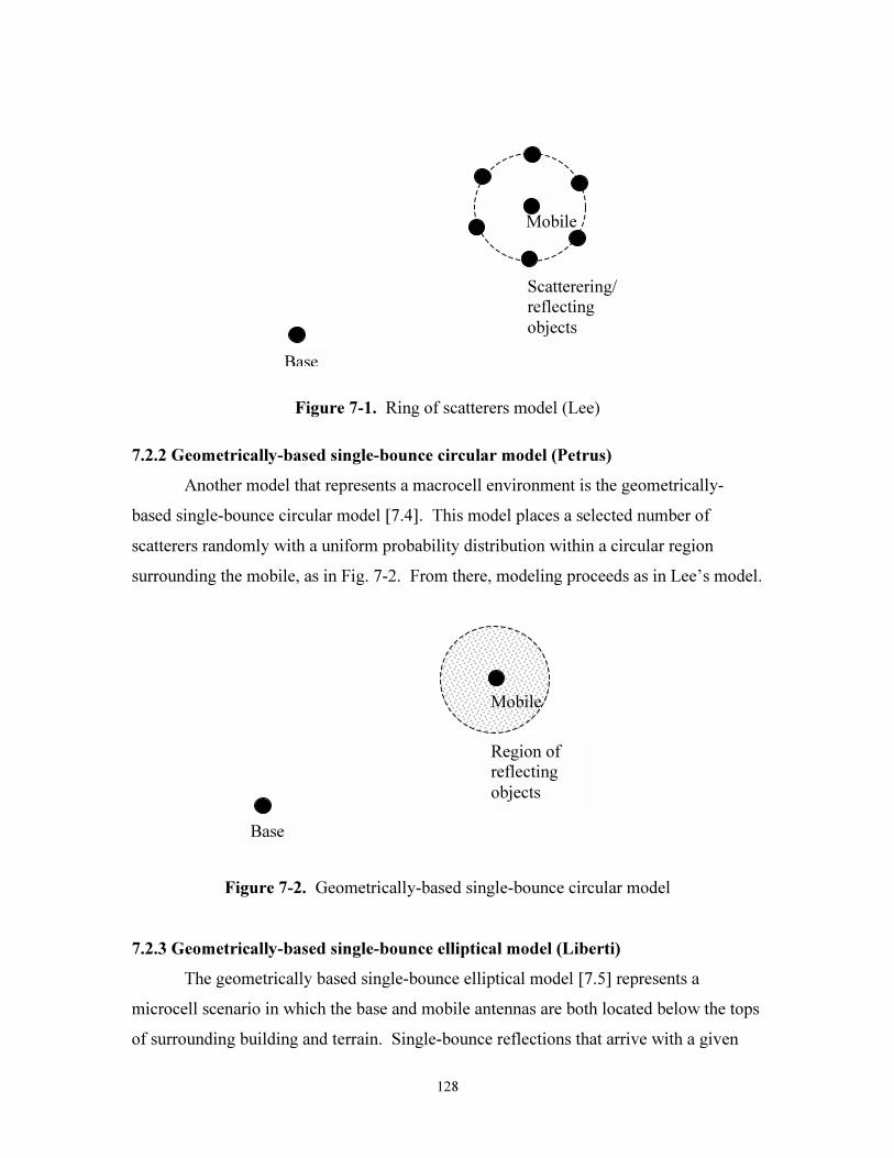
7.2.3 Geometrically-based single-bounce elliptical model (Liberti)

The geometrically based single-bounce elliptical model [7.5] represents a

microcell scenario in which the base and mobile antennas are both located below the tops

of surrounding building and terrain. Single-bounce reflections that arrive with a given

Mobile

Base

Scatterering/

reflecting

objects

Mobile

Base

Region of

reflecting

objects

129

delay are due to reflecting objects that lie on an ellipse that has its foci at the base and

mobile locations. In this model, reflectors are randomly located with a uniform

probability distribution within a region bounded by the ellipse that corresponds to the

maximum delay in the channel. Figure 7-3 shows this region of scatterers.

Figure 7-3. Geometrically-based single-bounce elliptical model

7.3 Reflection of Polarized Waves

The reflection of a polarized wave at a planar surface depends on the properties of

the material and on the angle of incidence and polarization of the incoming wave.

Because orthogonally polarized components of the wave are reflected differently,

reflection usually results in some depolarization of the wave.

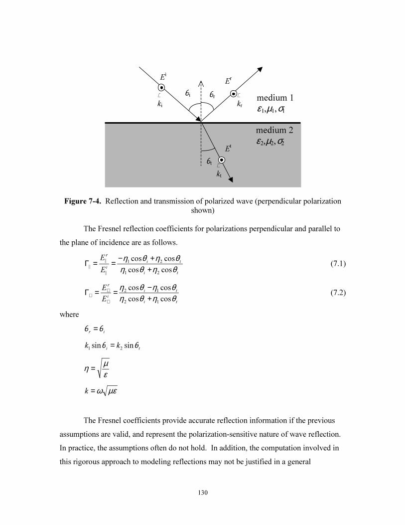
The Fresnel reflection coefficients [7.6] describe the reflection of polarized waves

at the planar interface of two dissimilar media, as shown in Fig. 7-4. The Fresnel

coefficients are based on the assumptions that the media and their interface are infinite in

extent, and that the interface is smooth. This is approximately true if irregularities in the

interface are much smaller than a wavelength, and the dimensions of the interface and the

depth of the media are much larger than a wavelength.

Mobile

Base

Region of

reflecting

objects

130

Figure 7-4. Reflection and transmission of polarized wave (perpendicular polarization

shown)

The Fresnel reflection coefficients for polarizations perpendicular and parallel to

the plane of incidence are as follows.

ti

ti

i

r

E

E

θηθηθηθη

coscos

coscos

21

21

||

||

|| ++−==Γ (7.1)

ti

ti

i

r

E

E

θηθηθηθη

coscos

coscos

12

12

+−==Γ

⊥

⊥⊥ (7.2)

where

irθθ =

tikk θθ sinsin21

=

εµη =

µεω=k

The Fresnel coefficients provide accurate reflection information if the previous

assumptions are valid, and represent the polarization-sensitive nature of wave reflection.

In practice, the assumptions often do not hold. In addition, the computation involved in

this rigorous approach to modeling reflections may not be justified in a general

θt ∧kt

θi θr

Ei

medium 2

ε2,µ2,σ2

medium 1

ε1,µ1,σ1

Et

Er

∧kr

∧ki

131

propagation model. An alternative is to use reflection coefficients that do not include

dependence on the angle of incidence. This introduces an approximation but requires less

computation. Constant reflection coefficients can be assumed to be the same or different

for different polarizations, and can be determined based on the mean of the Fresnel

coefficients or based on some empirical approach, as is often the case in ray-tracing

models. Reflection using constant reflection coefficients will introduce some

depolarization unless the transmitted wave has pure vertical or pure horizontal

polarization.

7.4 Geometric Components for Modeling Transmission and Reception of Polarized

Waves in a Mobile Communication System

To evaluate the performance of polarization diversity or polarization-sensitive

adaptive array systems, it is necessary to model the propagation environment and the

antenna patterns in a way that includes polarization information. Mobile radios generally

use vertically polarized antennas. Handsets typically use linearly polarized antennas, but

the orientation of the antenna is random. When the handset is held to the user’s ear, the

antenna is inclined approximately 60° from vertical, and the azimuth angle is random

with a uniform probability distribution, if the user is assumed to be equally likely to face

any direction.

It is useful to represent electric field antenna patterns in terms of vertical and

horizontal components for any antenna orientation. This section presents a three-

dimensional representation of the antenna pattern and procedures for rotating the pattern

and determining the vertical and horizontal components of the rotated pattern.

Modeling the reception of polarized waves in a multipath channel leads to a new

definition of polarization for multipath signals. This can be used to generate fading

envelopes for diversity systems or spatial-polarization signatures for adaptive arrays.

132

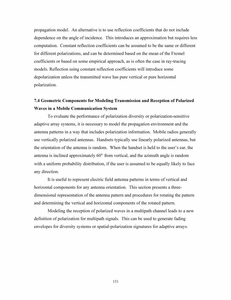
Figure 7-5. Coordinate systems for modeling transmission and reception of

polarized waves

7.4.1 Antenna pattern representation for polarization-sensitive channel modeling

To facilitate polarization-sensitive channel modeling, antenna patterns are

represented in three dimensions. Vertical and horizontal electric field component

patterns are sampled at regularly spaced angles θ and φ. This has been implemented in

MATLAB with the sampling resolution specified in degrees. Resolutions must be chosen

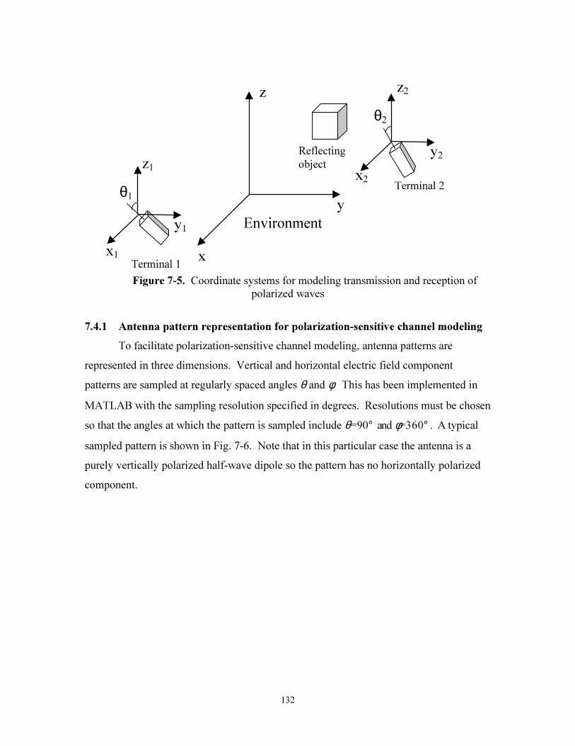
so that the angles at which the pattern is sampled include θ=90° and φ=360° . A typical

sampled pattern is shown in Fig. 7-6. Note that in this particular case the antenna is a

purely vertically polarized half-wave dipole so the pattern has no horizontally polarized

component.

x

y

z z2

x2z1

y1

x1

Terminal 2

Terminal 1

Environment

y2

θ2

θ1

Reflecting

object

133

Figure 7-6. Sampled 3-dimensional pattern of a vertical half-wave dipole with 10°

resolution in θ and φ. The pattern has no horizontally polarized component.

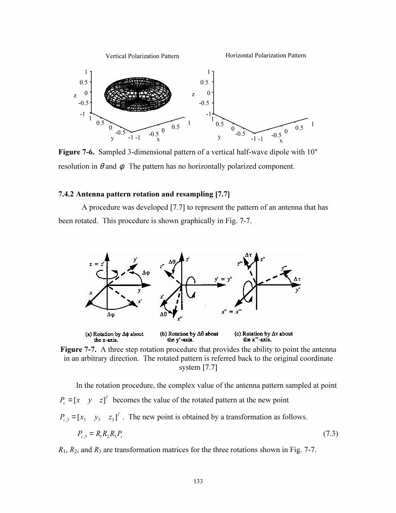
7.4.2 Antenna pattern rotation and resampling [7.7]

A procedure was developed [7.7] to represent the pattern of an antenna that has

been rotated. This procedure is shown graphically in Fig. 7-7.

Figure 7-7. A three step rotation procedure that provides the ability to point the antenna

in an arbitrary direction. The rotated pattern is referred back to the original coordinate

system [7.7]

In the rotation procedure, the complex value of the antenna pattern sampled at point

T

czyxP ][= becomes the value of the rotated pattern at the new point

T

czyxP ][ 3333, = . The new point is obtained by a transformation as follows.

ccPRRRP 3213, = (7.3)

R1, R2, and R3 are transformation matrices for the three rotations shown in Fig. 7-7.

-1-0.5

00.5

1

-1-0.5

0

1

xy

Vertical Polarization Pattern

-1-0.5

00.5

1

-1-0.5

00.5

1

-0.5

-1

0

0.5

1

x

z

Horizontal Polarization Pattern

-0.5

-1

0

0.5

1

0.5

z

y

134

The transformation matrices are

∆∆∆−∆

=100

0cossin

0sincos

1φφφφ

R (7.4)

∆∆−

∆∆=

θθ

θθ

cos0sin

010

sin0cos

2R (7.5)

∆∆∆−∆=ττττ

cossin0

sincos0

001

3R (7.6)

In spherical coordinates, the sampling points are Pc =(1,θ,φ) (before rotation) and

Pc, 3 =(1,θ ′′′ ,φ′′′ ) where the triple prime denotes the three rotations (∆φ,∆θ, and ∆τ ). The

original vertically and horizontally polarized patterns are rotated to obtain

),()(),()(

),()(),()(

,3,,

,3,,

φθφθφθφθ

HcHrotHcrotH

VcVrotVcrotV

fPffPf

fPffPf

==′′′′′′===′′′′′′=

(7.7)

The rotated patterns are then resampled at the nearest discrete points (θ,φ) determined by

the sampling resolution. The relationships between spherical and rectangular coordinates

are given by

=

+=

++=

−

−

x

y

z

yx

zyxr

1

22

1

222

tan

tan

φ

θ (7.8)

and

θφθφθ

cos

sinsin

cossin

rz

ry

rx

===

(7.9)

135

7.4.3 Antenna pattern repolarization

The pattern samples fV,rot(Pc3) and fH,rot(Pc3) obtained after rotating the pattern no

longer represent vertical and horizontal polarizations. It is relatively straightforward to

obtain the new vertically and horizontally polarized components of the rotated pattern,

and the procedure is described below. This procedure corresponds to Ludwig’s second

definition of cross polarization [7.8] and is also compatible with patterns obtained from

measurements using an azimuth-over-elevation positioner or from moment-method codes

such as NEC and WIRE.

All vectors shown in this procedure are represented in terms of the original basis

vectors [ ]Tx 001ˆ = , [ ]Ty 010ˆ = , and [ ]Tz 100ˆ = .

For a point Pc=(1,θ, φ) the unit vectors are given by

[ ]θφθφθ cossinsincossinˆ =r (7.10a)

rz

rz

ˆˆ

ˆˆˆ

××=φ (7.10b)

r

r

ˆˆ

ˆˆˆ

××=

φφθ (7.10c)

After rotation the new rectangular unit vectors are xRRRx ˆˆ321

=′′′ , yRRRy ˆˆ321

=′′′ , and

zRRRz ˆˆ321

=′′′ , where the triple prime denotes three rotations. The unit vector r is as

defined in (7.10a) above, and the other spherical unit vectors are

rz

rz

ˆˆ

ˆˆˆ

×′′′×′′′=′′′φ (7.11a)

r

r

ˆˆ

ˆˆˆ

×′′′×′′′=′′′

φφθ (7.11b)

The vertically polarized component of the rotated pattern ( the component in the θ

direction) and the horizontally polarized component (the component in the φdirection)

are given by

),(]ˆˆ[),(]ˆˆ[),(,,,

φθθφφθθθφθrotHrotVVrot

fff ⋅′′′+⋅′′′= (7.12a)

136

),(]ˆˆ[),(]ˆˆ[),(,,,

φθφφφθφθφθrotHrotVHrot

fff ⋅′′′+⋅′′′= (7.12b)

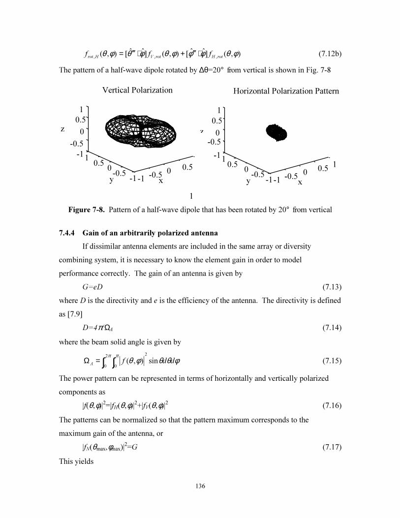
The pattern of a half-wave dipole rotated by ∆θ=20° from vertical is shown in Fig. 7-8

Figure 7-8. Pattern of a half-wave dipole that has been rotated by 20° from vertical

7.4.4 Gain of an arbitrarily polarized antenna

If dissimilar antenna elements are included in the same array or diversity

combining system, it is necessary to know the element gain in order to model

performance correctly. The gain of an antenna is given by

G=eD (7.13)

where D is the directivity and e is the efficiency of the antenna. The directivity is defined

as [7.9]

D=4π/ΩA (7.14)

where the beam solid angle is given by

∫ ∫=Ωπ π

φθθφθ2

0

2

0

sin),( ddfA

(7.15)

The power pattern can be represented in terms of horizontally and vertically polarized

components as

|f(θ,φ)|2=|fH(θ,φ)|

2+|fV(θ,φ)|

2(7.16)

The patterns can be normalized so that the pattern maximum corresponds to the

maximum gain of the antenna, or

|fN(θmax,φmax)|2=G (7.17)

This yields

1

-1 -0.50 0.5

-1-0.5

00.5

1-1

-0.5

0

0.5

1

xy

z

Vertical Polarization

-0.5

z

-1 -0.50

0.51

-1-0.5

00.5

1-1

0

0.5

1

xy

Horizontal Polarization Pattern

137

),(),(

),(maxmax

φθφθ

φθ ff

GfN

= (7.18)

If the antenna does not have pure polarization, then

),(),(

),(maxmax

,φθ

φθφθ

HNHf

f

Gf = (7.19a)

),(),(

),(maxmax

,φθ

φθφθ

VNVf

f

Gf = (7.19b)

Note that after the rotation procedure described in Sections 7.4.2 and 7.4.3, the gain will

be unchanged except for the error introduced by resampling the rotated pattern.

7.4.5 Polarization in Multipath Channels

Polarization states are well defined for plane waves. Because mobile radio

channels typically include multipath propagation, a new definition is needed for these

channels. Here three increasingly general definitions are presented that are applicable to

multipath channels.

The horizontally and vertically polarized components of a plane wave are

represented in phasor notation as follows [7.10]:

1EE

H= (7.20a)

δjV eEE

2= (7.20b)

where E1 and E2 are the amplitudes of the horizontal and vertical components,

respectively and δ is the phase of the vertically polarized part of the signal relative to the

horizontally polarized part. The absolute phase is omitted. This definition does not apply

in a multipath channel. The received signal in a multipath channel can be represented as

the superposition of M plane waves. In general, each of these plane waves can have a

different absolute phase, angle of arrival, and polarization state.

The following representation is independent of antenna pattern (or assumes

isotropic horizontally and vertically polarized patterns):

∑=

′′=M

i

j

Hi

i

eEE

1

1

δ(7.21a)

138

∑=

+′′=M

i

j

Vii

i

eEE

1

)(

2

δδ(7.21b)

E1i and E2i are the horizontal and vertical components of the ith

plane wave, respectively

and δi is the phase of the vertically polarized part of the ith

multipath component relative

to the horizontally polarized part.

If a receiver uses two antennas that are oriented vertically and horizontally, the

polarization can be defined in terms of the antenna response g(θ,φ,P) as:

∑=

′′=M

i

j

iiHi

i

eEHgE1

1),,(δφθ (7.22a)

∑=

+′′=M

i

j

iiVii

i

eEVgE1

)(

2),,(δδφθ (7.22b)

In the general case of three dimensions, up to three orthogonal polarizations are

possible. The polarization can be defined in terms of three polarizations as follows. In

this case the polarizations are not assumed to be horizontal and vertical.

∑=

′′=′M

i

j

iiPi

i

eEPgE1

11),,(

1

δφθ (7.23a)

∑=

+′′=′M

i

j

iiPii

i

eEPgE1

)(

222

2

),,(δδφθ (7.23b)

∑=

+′′=′M

i

j

iiPii

i

eEPgE1

)(

333

3

),,(δδφθ (7.23c)

7.5 Simulation of Polarization-Sensitive Multipath Propagation [7.11]

The Vector Multipath Propagation Simulator (VMPS) was developed to function

in conjunction with experimental measurements in either narrowband or wideband signal

environments. The complete radio channel can be modeled with this simulator including

antenna and propagation effects. Polarization is included in the models. The modeled

results can be used to confirm experimental results and visa versa. The goal is to study

and isolate the independent effects of such parameters as antenna pattern, polarization,

and spacing, multipath, interference, algorithm performance, and others. This section

draws extensively from a previous report on VMPS [7.11] but contains some additional

material.

139

7.5.1 Description of VMPS

The vector multipath propagation simulator (VMPS) is a two-dimensional

polarization-sensitive vector multipath channel modeling software tool that implements

many of the features described in this chapter. A receiver system with up to 8 antennas

can be modeled with the VMPS simulator. Up to 6 transmitters can be activated and

placed at arbitrary locations around the receiver. Any of these transmitters can be

selected to be the desired transmitter leaving the remaining activated transmitters as

sources of interference. Multipath is simulated through the addition of scatterers in the

propagation environment. The locations of scatterers seen by each transmitter are

determined using built in multipath models can be selected by the user. Manual

placement of scatterers is currently implemented for wideband simulations and will be

supported for narrowband simulations in future versions of VMPS. The power sent out

of each transmitter can be varied as well as two angle-independent reflection coefficients

(one each for vertically and horizontally polarized waves) that apply to all of the

scatterers associated with that transmitter. Additionally, the direct line of sight between

the receiver and a given transmitter can be turned off or on, simulating blocked or

unblocked line of sight. The combination of all these features allows for the simulation

of a wide variety of channel conditions.

VMPS includes both wideband and narrowband modeling. The narrowband

simulator can model the performance of receiving array configurations that include

spatial, polarization, and pattern or angle diversity. Performance of array configurations

with diversity combining as well as adaptive beamforming algorithms can be evaluated

using VMPS. The result is to establish the statistics of diversity gain or interference

rejection as a function of envelope correlation, multipath scenario, and antenna

configuration. The diversity gain can be established for one of the following combining

schemes: maximal ratio, selection, or equal gain combining. The diversity schemes are

applied to the received signal envelopes at the antenna elements of a moving receiver

within the propagation environment. A plot of the statistics of diversity gain and the

individual envelopes received at the antennas can be plotted for a user-defined

environment.

140

7.5.2 Simulation procedure

To simulate the performance of an adaptive array or diversity combining system

the procedure shown below is used:

1. Generate antenna pattern files for transmitting and receiving antenna elements

2. Generate array pattern file for transmitting terminal (if array is used at transmitter)

3. Specify terminal locations, multipath model parameters

4. Calculate spatial signature of desired and interfering signals

5. Generate received signal(s) if needed

6. Apply adaptive or diversity combining algorithm

7. Compare SNR or SINR before and after combining

The terminal locations are specified for each simulation and the scatterer locations

are determined using one of the models described in Section 7.2. The angles φ0, φ1i, and

φ2i are obtained directly from the system geometry, and the reflection angle φri can be

obtained from the other angles. From the system geometry and specification of the

antennas at each terminal, a spatial signature and/or instantaneous received signal

envelope can be obtained. By running consecutive simulations with one of the terminals

moving, time-varying spatial signatures or spatial-polarization signatures (described in

Chapter 3) and received signal envelopes can be obtained. These in turn can be used to

evaluate the performance of adaptive and diversity combining systems.

As with the receiver, the transmitter can be given an arbitrary antenna pattern. In

order to introduce multipath, scatterers (reflectors) can be introduced into to propagation

environment. A multipath component arrives from each scatterer location which can be

placed anywhere within the region. One of the built-in propagation models (Lee, Petrus,

Liberti) can also be used to randomly place scatterers within the environment (see

appendix). The number of scatterers as well as their reflection coefficients can be varied.

The version of VMPS used in this investigation represented used fixed scattering

coefficients and retained the same scatterer locations as the receiver or transmitter

moved. A newer version of VMPS that is currently being tested models specular

reflection implemented such that the initial reflection is assumed to occur at a point on a

planar surface. In the newer version of VMPS, the reflection point moves along the

141

surface as the receivers and/or transmitters moved so that the angles of incidence and

reflection are kept equal.

The received signal at each antenna is the sum of all signals arriving at the

antenna and the signal at each element can be combined using selection, equal gain, or

maximal ratio combining. A series of programs has been developed for simulating

polarization-sensitive multipath propagation. This software accounts for array geometry,

antenna gain, pattern, orientation, and polarization at the transmitting and receiving

terminals, and the multipath propagation environment. The simulation software allows

for arbitrary location of the two terminals. An example geometry shown in Fig. 7-9

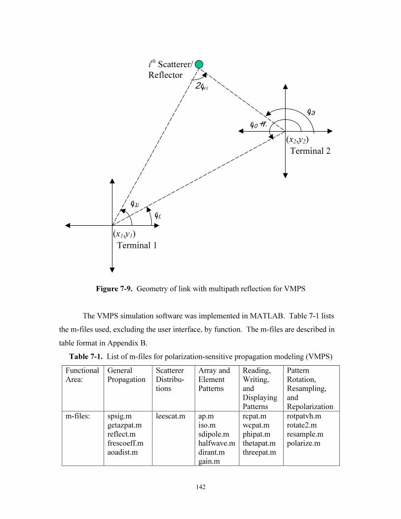
142

Figure 7-9. Geometry of link with multipath reflection for VMPS

The VMPS simulation software was implemented in MATLAB. Table 7-1 lists

the m-files used, excluding the user interface, by function. The m-files are described in

table format in Appendix B.

Table 7-1. List of m-files for polarization-sensitive propagation modeling (VMPS)

Functional

Area:

General

Propagation

Scatterer

Distribu-

tions

Array and

Element

Patterns

Reading,

Writing,

and

Displaying

Patterns

Pattern

Rotation,

Resampling,

and

Repolarization

m-files: spsig.m leescat.m ap.m rcpat.m rotpatvh.m

getazpat.m iso.m wcpat.m rotate2.m

reflect.m sdipole.m phipat.m resample.m

frescoeff.m halfwave.m thetapat.m polarize.m

aoadist.m dirant.m threepat.m

gain.m

φ0

φ1i

φ2ι

2φri

φ0 +π

(x1,y1)

(x2,y2)

Terminal 1

Terminal 2

ith

Scatterer/

Reflector

143

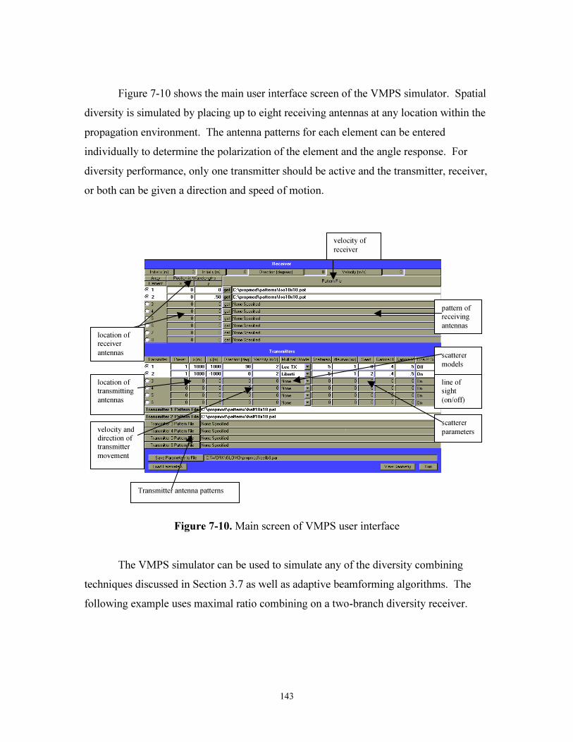
Figure 7-10 shows the main user interface screen of the VMPS simulator. Spatial

diversity is simulated by placing up to eight receiving antennas at any location within the

propagation environment. The antenna patterns for each element can be entered

individually to determine the polarization of the element and the angle response. For

diversity performance, only one transmitter should be active and the transmitter, receiver,

or both can be given a direction and speed of motion.

location ofreceiver

antennas

pattern ofreceiving

antennas

location of

transmitting

antennas

velocity and

direction oftransmitter

movement

scatterer

models

scatterer

parameters

Transmitter antenna patterns

velocity of

receiver

line of

sight

(on/off)

Figure 7-10. Main screen of VMPS user interface

The VMPS simulator can be used to simulate any of the diversity combining

techniques discussed in Section 3.7 as well as adaptive beamforming algorithms. The

following example uses maximal ratio combining on a two-branch diversity receiver.

144

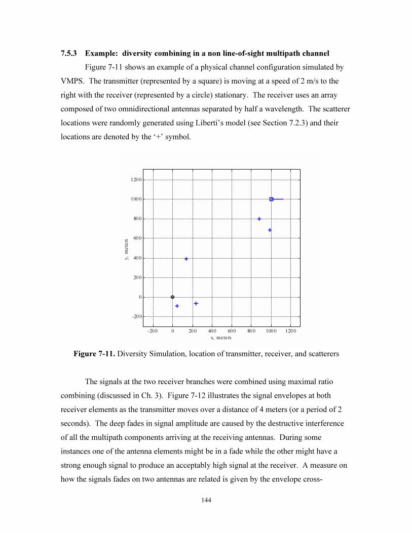
7.5.3 Example: diversity combining in a non line-of-sight multipath channel

Figure 7-11 shows an example of a physical channel configuration simulated by

VMPS. The transmitter (represented by a square) is moving at a speed of 2 m/s to the

right with the receiver (represented by a circle) stationary. The receiver uses an array

composed of two omnidirectional antennas separated by half a wavelength. The scatterer

locations were randomly generated using Liberti’s model (see Section 7.2.3) and their

locations are denoted by the ‘+’ symbol.

Figure 7-11. Diversity Simulation, location of transmitter, receiver, and scatterers

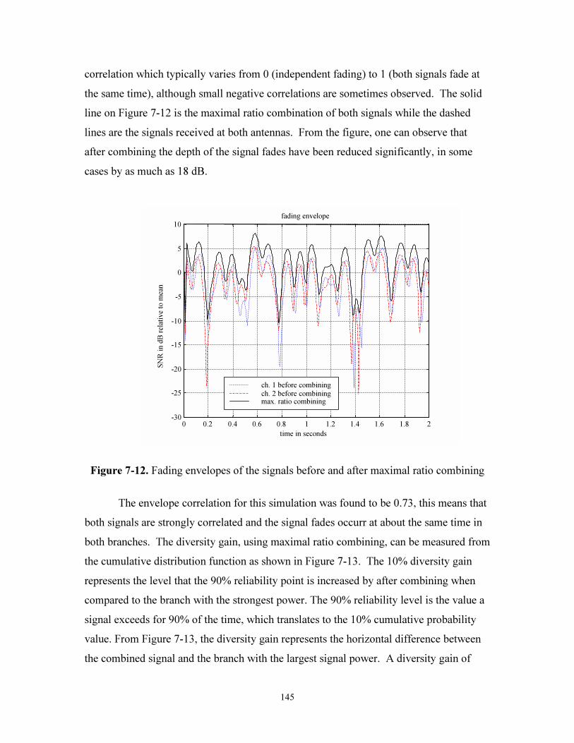
The signals at the two receiver branches were combined using maximal ratio

combining (discussed in Ch. 3). Figure 7-12 illustrates the signal envelopes at both

receiver elements as the transmitter moves over a distance of 4 meters (or a period of 2

seconds). The deep fades in signal amplitude are caused by the destructive interference

of all the multipath components arriving at the receiving antennas. During some

instances one of the antenna elements might be in a fade while the other might have a

strong enough signal to produce an acceptably high signal at the receiver. A measure on

how the signals fades on two antennas are related is given by the envelope cross-

-200 0 200 400 600 800 1000 1200

-200

0

200

400

600

800

1000

1200

x, meters

y,

me

ters

145

correlation which typically varies from 0 (independent fading) to 1 (both signals fade at

the same time), although small negative correlations are sometimes observed. The solid

line on Figure 7-12 is the maximal ratio combination of both signals while the dashed

lines are the signals received at both antennas. From the figure, one can observe that

after combining the depth of the signal fades have been reduced significantly, in some

cases by as much as 18 dB.

Figure 7-12. Fading envelopes of the signals before and after maximal ratio combining

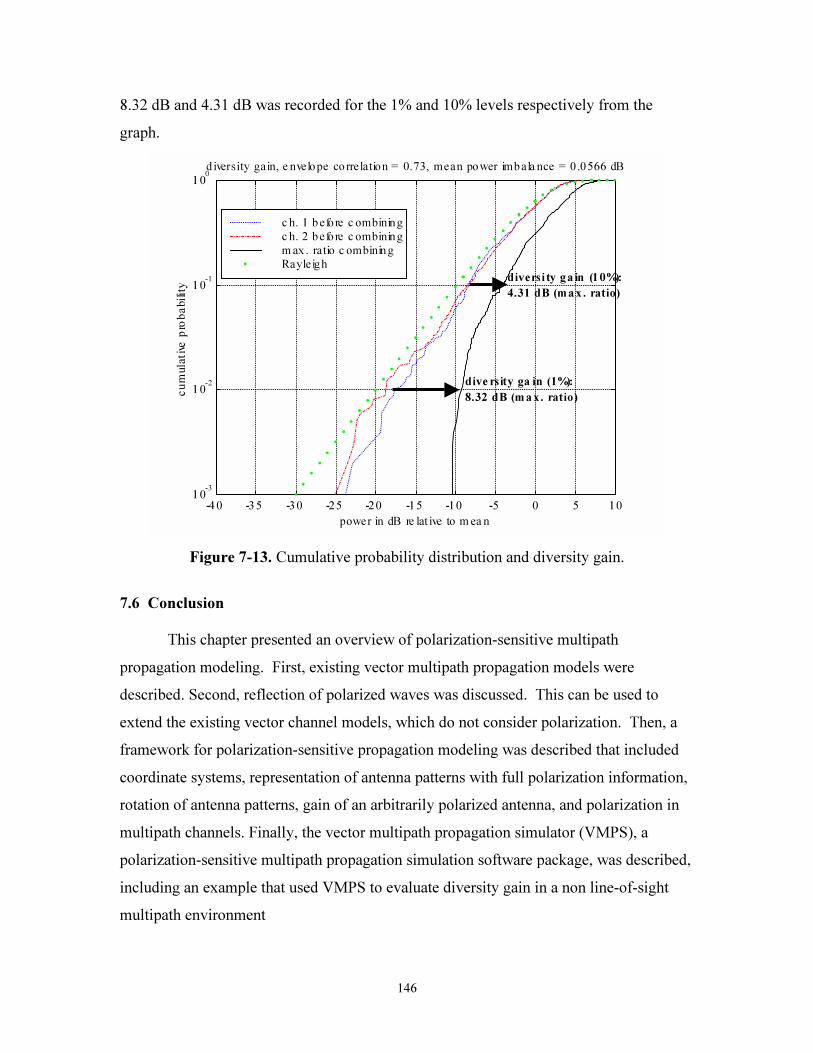
The envelope correlation for this simulation was found to be 0.73, this means that

both signals are strongly correlated and the signal fades occurr at about the same time in

both branches. The diversity gain, using maximal ratio combining, can be measured from

the cumulative distribution function as shown in Figure 7-13. The 10% diversity gain

represents the level that the 90% reliability point is increased by after combining when

compared to the branch with the strongest power. The 90% reliability level is the value a

signal exceeds for 90% of the time, which translates to the 10% cumulative probability

value. From Figure 7-13, the diversity gain represents the horizontal difference between

the combined signal and the branch with the largest signal power. A diversity gain of

0 0.2 0.4 0.6 0.8 1 1.2 1.4 1.6 1.8 2-30

-25

-20

-15

-10

-5

0

5

10fading envelope

time in seconds

SN

R i

n d

B r

ela

tive t

o m

ean

ch. 1 before combiningch. 2 before combiningmax. ratio combining

146

8.32 dB and 4.31 dB was recorded for the 1% and 10% levels respectively from the

graph.

-40 -35 -30 -25 -20 -15 -10 -5 0 5 1010

-3

10-2

10-1

100diversity gain, e nvelope co rrelation = 0.73, mean power imbala nce = 0 .0566 dB

power in dB re lat ive to m ea n

cu

mula

tive

pro

ba

bili

ty

diversi ty ga in (10%):

4.31 dB (max. ratio)

dive rsity ga in (1%):

8.32 dB (m ax. ratio)

c h. 1 before c ombining

c h. 2 before c ombining

m ax . ratio c ombining

Rayleigh

Figure 7-13. Cumulative probability distribution and diversity gain.

7.6 Conclusion

This chapter presented an overview of polarization-sensitive multipath

propagation modeling. First, existing vector multipath propagation models were

described. Second, reflection of polarized waves was discussed. This can be used to

extend the existing vector channel models, which do not consider polarization. Then, a

framework for polarization-sensitive propagation modeling was described that included

coordinate systems, representation of antenna patterns with full polarization information,

rotation of antenna patterns, gain of an arbitrarily polarized antenna, and polarization in

multipath channels. Finally, the vector multipath propagation simulator (VMPS), a

polarization-sensitive multipath propagation simulation software package, was described,

including an example that used VMPS to evaluate diversity gain in a non line-of-sight

multipath environment

147

References

[7.1] R. B. Ertel, et al., “Overview of Spatial Channel Models for Antenna Array

Communication Systems,” IEEE Personal Communications, pp. 10-22, February

1998.

[7.2] S. Y. Seidel and T. S. Rappaport, “Site-specific propagation prediction for wireless

in-building personal communication system design,” IEEE Transactions on

Vehicular Technology, vol.43, no.4, Nov. 1994, pp.879-91.

[7.3] W. C. Y. Lee, Mobile Communications Engineering, McGraw Hill, New York,

1982.

[7.4] P. Petrus, J. H. Reed, and T. S. Rappaport, “Geometrically Based Statistical

Channel Model for Macrocellular Mobile Environments,” IEEE GLOBECOM,

Vol. 2, pp. 1197-1201, 1996.

[7.5] J. C. Liberti and T. S. Rappaport, “A Geometrically Based Model for Line-of-

Sight Multipath Radio Channels,” IEEE Vehicular Technology Conference, Vol. 2,

pp. 844-848, 1996.

[7.6] C. A. Balanis, Advanced Engineering Electromagnetics, John Wiley & Sons,

1989.

[7.7] J. C. Liberti, “Antenna File Formats for SISP,” Draft Report for MPRG, Virginia

Tech, September 6, 1994.

[7.8] A. C. Ludwig, “The Definition of Cross Polarization,” IEEE Transactions on

Antennas and Propagation, Vol. AP-21, pp. 116-119, Jan. 1973

[7.9] W. L. Stutzman and G. A. Thiele, Antenna Theory and Design, John Wiley &

Sons, New York, 1981.

[7.10] W. L. Stutzman, Polarization in Electromagnetic Systems, Artech House,

Norwood, MA, 1993.

[7.11] Kai Dietze, Carl Dietrich, and Warren Stutzman, Vector Multipath Propagation

Simulator (VMPS), Draft report, Virginia Tech Antenna Group, April 7, 1999.