chapter 7: derivation of discrete probability distributions · chapter 7: derivation of discrete...
TRANSCRIPT

Chapter 7: Derivation of Discrete ProbabilityDistributions
James B.Ramsey
Department of Economics, NYU
October 2007
(Institute) Chapter 7 October 2007 1 / 33

Explore Relationship Between Experiment & Prob. Distn.
So far all our probability distributions have started with probs.of elementary events under the equally likely principle.
We now derive more interesting distributions & relate the shapeof the prob. distribution to the details of the experiment.
(Institute) Chapter 7 October 2007 2 / 33

An Aside on Permutations & Combinations
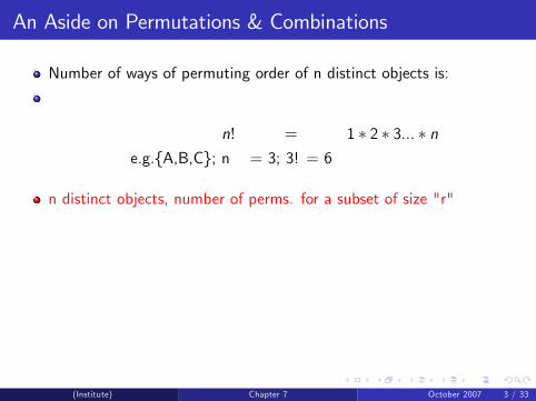
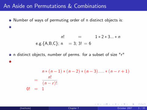
Number of ways of permuting order of n distinct objects is:
n! = 1 � 2 � 3... � ne.g.{A,B,C}; n = 3; 3! = 6
n distinct objects, number of perms. for a subset of size "r"
n � (n� 1) � (n� 2) � (n� 3)..... � (n� r + 1)
=n!
(n� r)!0! = 1
(Institute) Chapter 7 October 2007 3 / 33

An Aside on Permutations & Combinations
Number of ways of permuting order of n distinct objects is:
n! = 1 � 2 � 3... � ne.g.{A,B,C}; n = 3; 3! = 6
n distinct objects, number of perms. for a subset of size "r"
n � (n� 1) � (n� 2) � (n� 3)..... � (n� r + 1)
=n!
(n� r)!0! = 1
(Institute) Chapter 7 October 2007 3 / 33

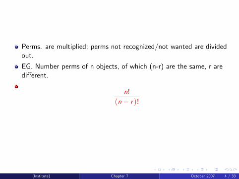
Perms. are multiplied; perms not recognized/not wanted are dividedout.
EG. Number perms of n objects, of which (n-r) are the same, r aredi¤erent.
n!(n� r)!
(Institute) Chapter 7 October 2007 4 / 33
Perms. are multiplied; perms not recognized/not wanted are dividedout.
EG. Number perms of n objects, of which (n-r) are the same, r aredi¤erent.
n!(n� r)!
(Institute) Chapter 7 October 2007 4 / 33
Perms. are multiplied; perms not recognized/not wanted are dividedout.
EG. Number perms of n objects, of which (n-r) are the same, r aredi¤erent.
n!(n� r)!
(Institute) Chapter 7 October 2007 4 / 33

Perms. & Combinations continued
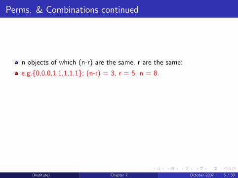
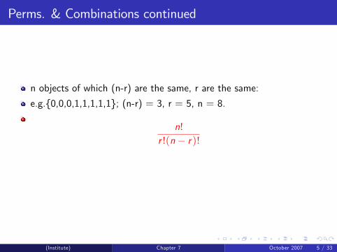
n objects of which (n-r) are the same, r are the same:
e.g.{0,0,0,1,1,1,1,1}; (n-r) = 3, r = 5, n = 8.
n!r !(n� r)!
Swap de�nition of which terms are (n-r), r to get same result.
(Institute) Chapter 7 October 2007 5 / 33
Perms. & Combinations continued
n objects of which (n-r) are the same, r are the same:
e.g.{0,0,0,1,1,1,1,1}; (n-r) = 3, r = 5, n = 8.
n!r !(n� r)!
Swap de�nition of which terms are (n-r), r to get same result.
(Institute) Chapter 7 October 2007 5 / 33
Perms. & Combinations continued
n objects of which (n-r) are the same, r are the same:
e.g.{0,0,0,1,1,1,1,1}; (n-r) = 3, r = 5, n = 8.
n!r !(n� r)!
Swap de�nition of which terms are (n-r), r to get same result.
(Institute) Chapter 7 October 2007 5 / 33

Perms. & Combinations continued
n objects of which (n-r) are the same, r are the same:
e.g.{0,0,0,1,1,1,1,1}; (n-r) = 3, r = 5, n = 8.
n!r !(n� r)!
Swap de�nition of which terms are (n-r), r to get same result.
(Institute) Chapter 7 October 2007 5 / 33

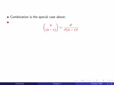
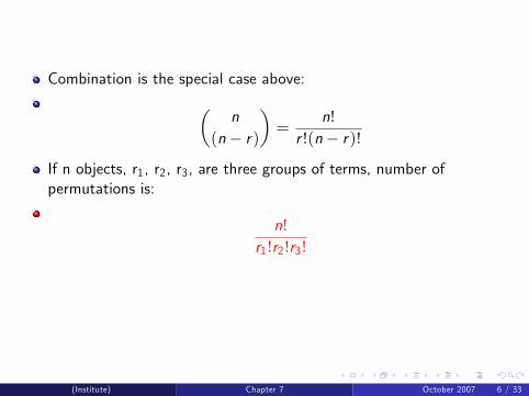
Combination is the special case above:
�n
(n� r)
�=
n!r !(n� r)!
If n objects, r1, r2, r3, are three groups of terms, number ofpermutations is:
n!r1!r2!r3!
n = ∑i ri .
(Institute) Chapter 7 October 2007 6 / 33
Combination is the special case above:�n
(n� r)
�=
n!r !(n� r)!
If n objects, r1, r2, r3, are three groups of terms, number ofpermutations is:
n!r1!r2!r3!
n = ∑i ri .
(Institute) Chapter 7 October 2007 6 / 33

Combination is the special case above:�n
(n� r)
�=
n!r !(n� r)!
If n objects, r1, r2, r3, are three groups of terms, number ofpermutations is:
n!r1!r2!r3!
n = ∑i ri .
(Institute) Chapter 7 October 2007 6 / 33
Combination is the special case above:�n
(n� r)
�=
n!r !(n� r)!
If n objects, r1, r2, r3, are three groups of terms, number ofpermutations is:
n!r1!r2!r3!
n = ∑i ri .
(Institute) Chapter 7 October 2007 6 / 33

Combination is the special case above:�n
(n� r)
�=
n!r !(n� r)!
If n objects, r1, r2, r3, are three groups of terms, number ofpermutations is:
n!r1!r2!r3!
n = ∑i ri .
(Institute) Chapter 7 October 2007 6 / 33
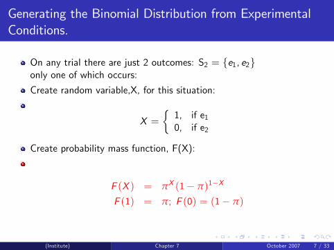
Generating the Binomial Distribution from ExperimentalConditions.
On any trial there are just 2 outcomes: S2 = fe1, e2gonly one of which occurs:
Create random variable,X, for this situation:
X =�1, if e10, if e2
Create probability mass function, F(X):
F (X ) = πX (1� π)1�X
F (1) = π; F (0) = (1� π)
(Institute) Chapter 7 October 2007 7 / 33

Binomial Generation continued:
Now consider a sequence of n, independent trials with constant π.
On each trial record as outcome: {0, or 1}.
We seek probability of getting K successes [1�s] in n trials.
Probability distribution for n trials is by independence:
Fj (X1,X2, ....Xn) = ∏iF (Xi )
= ∏i
πXi (1� π)1�Xi
(Institute) Chapter 7 October 2007 8 / 33

Aside on "convolution sum" as used above for getting K successes.Let Xi = {0, 1}, i = 1,2,3 and independent; range of Xi is {0,1}.Let Y � ∑i Xi , convolution sum, then the range of Y values is {0,1,2,3}
(Institute) Chapter 7 October 2007 9 / 33

What is the probability of K successes in n independenttrials?
Consider �rst the prob. of K successes in some given �xed order: e.g.
f1, 1, 0, 1, 0gK = 3, n = 5
Probability of this joint event is:
F (X1 = 1,X2 = 1,X3 = 0,X4 = 1,X5 = 0)
= π � π � (1� π) � π � (1� π)
= π3 � (1� π)2
(Institute) Chapter 7 October 2007 10 / 33
Each sequence containing three 1�s and two 0�s is mutually exclusiveto anothersequence with the same number of 1�s & 0�s
We can add the probabilities; question is how many such sequencesare there?We have out of �ve trials, three 1�s & 2 0�s, so answer is:�
53
�=
5!3!2!
= 10
And the probability is given by:(for given value of π)
10 � π3 � (1� π)2
= 10 � (12)5 = 0.3125
for π =1/2
= 10 � (3/8)3 � (5/8)2 = 0.206for π = 3/8
(Institute) Chapter 7 October 2007 11 / 33
Each sequence containing three 1�s and two 0�s is mutually exclusiveto anothersequence with the same number of 1�s & 0�sWe can add the probabilities; question is how many such sequencesare there?
We have out of �ve trials, three 1�s & 2 0�s, so answer is:�53
�=
5!3!2!
= 10
And the probability is given by:(for given value of π)
10 � π3 � (1� π)2
= 10 � (12)5 = 0.3125
for π =1/2
= 10 � (3/8)3 � (5/8)2 = 0.206for π = 3/8
(Institute) Chapter 7 October 2007 11 / 33
Each sequence containing three 1�s and two 0�s is mutually exclusiveto anothersequence with the same number of 1�s & 0�sWe can add the probabilities; question is how many such sequencesare there?We have out of �ve trials, three 1�s & 2 0�s, so answer is:
�53
�=
5!3!2!
= 10
And the probability is given by:(for given value of π)
10 � π3 � (1� π)2
= 10 � (12)5 = 0.3125
for π =1/2
= 10 � (3/8)3 � (5/8)2 = 0.206for π = 3/8
(Institute) Chapter 7 October 2007 11 / 33

Each sequence containing three 1�s and two 0�s is mutually exclusiveto anothersequence with the same number of 1�s & 0�sWe can add the probabilities; question is how many such sequencesare there?We have out of �ve trials, three 1�s & 2 0�s, so answer is:�
53
�=
5!3!2!
= 10
And the probability is given by:(for given value of π)
10 � π3 � (1� π)2
= 10 � (12)5 = 0.3125
for π =1/2
= 10 � (3/8)3 � (5/8)2 = 0.206for π = 3/8
(Institute) Chapter 7 October 2007 11 / 33

De�nition of the Binomial Distribution
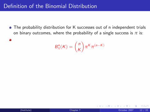
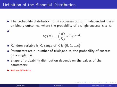
The probability distribution for K successes out of n independent trialson binary outcomes, where the probability of a single success is π is:
Bnπ(K ) =�nK
�πKπ(n�K )
Random variable is K, range of K is {0, 1, ...n}
Parameters are n, number of trials,and π, the probability of successon a single trial.
Shape of probability distribution depends on the values of theparameters;
see overheads.
(Institute) Chapter 7 October 2007 12 / 33
De�nition of the Binomial Distribution
The probability distribution for K successes out of n independent trialson binary outcomes, where the probability of a single success is π is:
Bnπ(K ) =�nK
�πKπ(n�K )
Random variable is K, range of K is {0, 1, ...n}
Parameters are n, number of trials,and π, the probability of successon a single trial.
Shape of probability distribution depends on the values of theparameters;
see overheads.
(Institute) Chapter 7 October 2007 12 / 33
Do the Binomial Probabilities Sum to One?
Consider the expansion:
(π + (1� π))n =n
∑0
�nK
�πK (1� π)n�K = 1n = 1
Recall Pascal�s Triangle for the coe¢ cients in a bivariate expansion:(a+b)n.
11 1
1 2 11 3 3 1
(Institute) Chapter 7 October 2007 13 / 33

Do the Binomial Probabilities Sum to One?
Consider the expansion:
(π + (1� π))n =n
∑0
�nK
�πK (1� π)n�K = 1n = 1
Recall Pascal�s Triangle for the coe¢ cients in a bivariate expansion:(a+b)n.
11 1
1 2 11 3 3 1
(Institute) Chapter 7 October 2007 13 / 33

Do the Binomial Probabilities Sum to One?
Consider the expansion:
(π + (1� π))n =n
∑0
�nK
�πK (1� π)n�K = 1n = 1
Recall Pascal�s Triangle for the coe¢ cients in a bivariate expansion:(a+b)n.
11 1
1 2 11 3 3 1
(Institute) Chapter 7 October 2007 13 / 33

Do the Binomial Probabilities Sum to One?
Consider the expansion:
(π + (1� π))n =n
∑0
�nK
�πK (1� π)n�K = 1n = 1
Recall Pascal�s Triangle for the coe¢ cients in a bivariate expansion:(a+b)n.
11 1
1 2 11 3 3 1
(Institute) Chapter 7 October 2007 13 / 33

Theoretical Moments
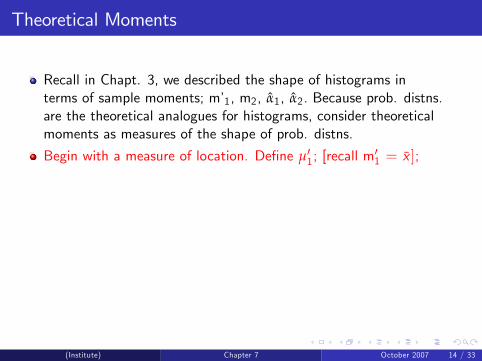
Recall in Chapt. 3, we described the shape of histograms interms of sample moments; m�1, m2, α̂1, α̂2. Because prob. distns.are the theoretical analogues for histograms, consider theoreticalmoments as measures of the shape of prob. distns.
Begin with a measure of location. De�ne µ01; [recall m01 = x̄ ];
µ01(X ) =n
∑1XiP(Xi )
if P(Xi ) = 1/nlink to m1�is clear.
(Institute) Chapter 7 October 2007 14 / 33
Theoretical Moments
Recall in Chapt. 3, we described the shape of histograms interms of sample moments; m�1, m2, α̂1, α̂2. Because prob. distns.are the theoretical analogues for histograms, consider theoreticalmoments as measures of the shape of prob. distns.
Begin with a measure of location. De�ne µ01; [recall m01 = x̄ ];
µ01(X ) =n
∑1XiP(Xi )
if P(Xi ) = 1/nlink to m1�is clear.
(Institute) Chapter 7 October 2007 14 / 33

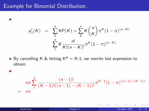
Example for Binomial Distribution.
µ01(K ) =n
∑0KP(K ) =
n
∑0K�nK
�πK (1� π)(n�K )
n
∑1K
n!K !(n�K )! πK (1� π)(n�K )
By cancelling K & letting K* = K-1; we rewrite last expression toobtain:
nπn
∑1
(n� 1)!(K � 1)!((n� 1)� (K � 1))! πK�1(1� π)((n�1)�(K�1))
= nπ
(Institute) Chapter 7 October 2007 15 / 33

Measure of "spread". We de�ne:
µ2(K ) = ∑(K � µ01)2P(K )
= nπ(1� π) = nπq
q = (1� π)
(Institute) Chapter 7 October 2007 16 / 33

Measure of Symmetry;we de�ne:
µ3(K ) = ∑(K � µ01)3P(K )
= nπq(1� 2π)
And a measure of peakedness, or of fat tails:
µ4(K ) = ∑(K � µ01)4P(K )
= 3(nπq)2 + nπq(1� 6πq)
(Institute) Chapter 7 October 2007 17 / 33

Measure of Symmetry;we de�ne:
µ3(K ) = ∑(K � µ01)3P(K )
= nπq(1� 2π)
And a measure of peakedness, or of fat tails:
µ4(K ) = ∑(K � µ01)4P(K )
= 3(nπq)2 + nπq(1� 6πq)
(Institute) Chapter 7 October 2007 17 / 33

Measure of Symmetry;we de�ne:
µ3(K ) = ∑(K � µ01)3P(K )
= nπq(1� 2π)
And a measure of peakedness, or of fat tails:
µ4(K ) = ∑(K � µ01)4P(K )
= 3(nπq)2 + nπq(1� 6πq)
(Institute) Chapter 7 October 2007 17 / 33

We standardize the third & fourth moments to obtain:
α1(K ) =nπq(1� 2π)
(nπq)3/2
=(1� 2π)pnπq
α2(K ) =3(nπq)2 + nπq(1� 6πq)
(nπq)2
= 3+(1� 6πq)(nπq)
(Institute) Chapter 7 October 2007 18 / 33

We standardize the third & fourth moments to obtain:
α1(K ) =nπq(1� 2π)
(nπq)3/2
=(1� 2π)pnπq
α2(K ) =3(nπq)2 + nπq(1� 6πq)
(nπq)2
= 3+(1� 6πq)(nπq)
(Institute) Chapter 7 October 2007 18 / 33

We can take limits of the standardized moments as n ) ∞.
limn)∞
(α1) = limn)∞
((1� 2π)pnπq
)
= 0
limn)∞
(α2) = limn)∞
(3+(1� 6πq)(nπq)
)
= 3
(Institute) Chapter 7 October 2007 19 / 33

We can take limits of the standardized moments as n ) ∞.
limn)∞
(α1) = limn)∞
((1� 2π)pnπq
)
= 0
limn)∞
(α2) = limn)∞
(3+(1� 6πq)(nπq)
)
= 3
(Institute) Chapter 7 October 2007 19 / 33

We can take limits of the standardized moments as n ) ∞.
limn)∞
(α1) = limn)∞
((1� 2π)pnπq
)
= 0
limn)∞
(α2) = limn)∞
(3+(1� 6πq)(nπq)
)
= 3
(Institute) Chapter 7 October 2007 19 / 33
Explore the shape of the prob. distn. as a function of "n" & π; seeoverheads.
NOTE: notice Greek characters for parameters of the prob. distns.& no hats on α1, α2.
Parameters determine shape of prob. distn.;moments as functions of the parameters reveal shape of prob. distn.;conditions of the experiment determine the values of the parameters.
Remember that random variables are theoretical entities &ALWAYS have associated with them a probability distribution.
(Institute) Chapter 7 October 2007 20 / 33

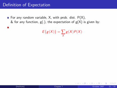
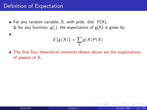
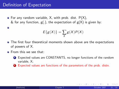
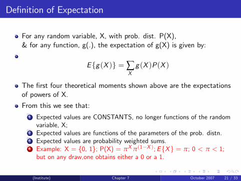
De�nition of Expectation
For any random variable, X, with prob. dist. P(X),& for any function, g(.), the expectation of g(X) is given by:
Efg(X )g = ∑X
g(X )P(X )
The �rst four theoretical moments shown above are the expectationsof powers of X.
From this we see that:
1 Expected values are CONSTANTS, no longer functions of the randomvariable, X;
2 Expected values are functions of the parameters of the prob. distn.3 Expected values are probability weighted sums.4 Example: X = {0, 1}; P(X) = πXπ(1�X );EfXg = π; 0 < π < 1;but on any draw,one obtains either a 0 or a 1.
(Institute) Chapter 7 October 2007 21 / 33

De�nition of Expectation
For any random variable, X, with prob. dist. P(X),& for any function, g(.), the expectation of g(X) is given by:
Efg(X )g = ∑X
g(X )P(X )
The �rst four theoretical moments shown above are the expectationsof powers of X.
From this we see that:1 Expected values are CONSTANTS, no longer functions of the randomvariable, X;
2 Expected values are functions of the parameters of the prob. distn.3 Expected values are probability weighted sums.4 Example: X = {0, 1}; P(X) = πXπ(1�X );EfXg = π; 0 < π < 1;but on any draw,one obtains either a 0 or a 1.
(Institute) Chapter 7 October 2007 21 / 33
De�nition of Expectation
For any random variable, X, with prob. dist. P(X),& for any function, g(.), the expectation of g(X) is given by:
Efg(X )g = ∑X
g(X )P(X )
The �rst four theoretical moments shown above are the expectationsof powers of X.
From this we see that:1 Expected values are CONSTANTS, no longer functions of the randomvariable, X;
2 Expected values are functions of the parameters of the prob. distn.
3 Expected values are probability weighted sums.4 Example: X = {0, 1}; P(X) = πXπ(1�X );EfXg = π; 0 < π < 1;but on any draw,one obtains either a 0 or a 1.
(Institute) Chapter 7 October 2007 21 / 33

De�nition of Expectation
For any random variable, X, with prob. dist. P(X),& for any function, g(.), the expectation of g(X) is given by:
Efg(X )g = ∑X
g(X )P(X )
The �rst four theoretical moments shown above are the expectationsof powers of X.
From this we see that:1 Expected values are CONSTANTS, no longer functions of the randomvariable, X;
2 Expected values are functions of the parameters of the prob. distn.3 Expected values are probability weighted sums.
4 Example: X = {0, 1}; P(X) = πXπ(1�X );EfXg = π; 0 < π < 1;but on any draw,one obtains either a 0 or a 1.
(Institute) Chapter 7 October 2007 21 / 33
De�nition of Expectation
For any random variable, X, with prob. dist. P(X),& for any function, g(.), the expectation of g(X) is given by:
Efg(X )g = ∑X
g(X )P(X )
The �rst four theoretical moments shown above are the expectationsof powers of X.
From this we see that:1 Expected values are CONSTANTS, no longer functions of the randomvariable, X;
2 Expected values are functions of the parameters of the prob. distn.3 Expected values are probability weighted sums.4 Example: X = {0, 1}; P(X) = πXπ(1�X );EfXg = π; 0 < π < 1;but on any draw,one obtains either a 0 or a 1.
(Institute) Chapter 7 October 2007 21 / 33

Properties of the Expectation Operator
If Y = a +bX, E{Y} = a +bE{X}.
If Y = a1X1 + a2X2; F(X1, X2) is the joint distribution of {X1, X2}:
EfY g = a1 ∑X2, X1
X1F (X1,X2) + a2 ∑X1,X2
X2F (X1,X2)
= a1 ∑X1
X1FX1(X1) + a2 ∑X2
X2FX2(X2)
= a1EfX1g+ a2EfX2gFX1(X1) = ∑
X2
F (X1,X2), FX2(X2) = ∑X1
F (X1,X2)
(Institute) Chapter 7 October 2007 22 / 33
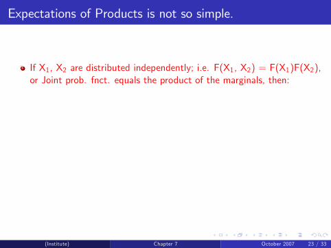
Expectations of Products is not so simple.
If X1, X2 are distributed independently; i.e. F(X1, X2) = F(X1)F(X2),or Joint prob. fnct. equals the product of the marginals, then:
EfX1 � X2g = ∑X1, X2
[X1 � X2]F (X1) � F (X2)
= ∑X1
[X1F (X1)]∑X2
[X2F (X2)]
= EfX1g � EfX2g
(Institute) Chapter 7 October 2007 23 / 33

But if the joint distn. is not the product of the marginals:
FjfX1, X2g 6= F (X1) � F (X2), but does equal conditional * marginal,or:
FjfX1, X2g = FfX2 j X1gFfX1g
EfX1X2g = ∑X1
X1
"∑X2
X2FfX2 j X1g#FfX1g
= ∑X1
X1G (X1)FfX1g 6= EfX1g � EfX2g
(Institute) Chapter 7 October 2007 24 / 33

But if the joint distn. is not the product of the marginals:
FjfX1, X2g 6= F (X1) � F (X2), but does equal conditional * marginal,or:
FjfX1, X2g = FfX2 j X1gFfX1g
EfX1X2g = ∑X1
X1
"∑X2
X2FfX2 j X1g#FfX1g
= ∑X1
X1G (X1)FfX1g 6= EfX1g � EfX2g
(Institute) Chapter 7 October 2007 24 / 33

Functions of Random Variables are Random Variables
Let X be a random var. with prob. fnct. F(X) & let g(X) be a 1-1fnct.,then Y = g(X) has a prob. distn. fnct. H(Y) & E{Y} = E{g(X)}.
If Y = g(X) & g(.) is 1-1;X = g�1(Y )
Efg(X )g = ∑X
g(X )F (X )
= ∑Y
YF (g�1(Y )
= ∑Y
YH(Y ) = EfY g
H(Y ) = F (g�1(Y )
(Institute) Chapter 7 October 2007 25 / 33

Derivation of the Poisson Probability Distribution.
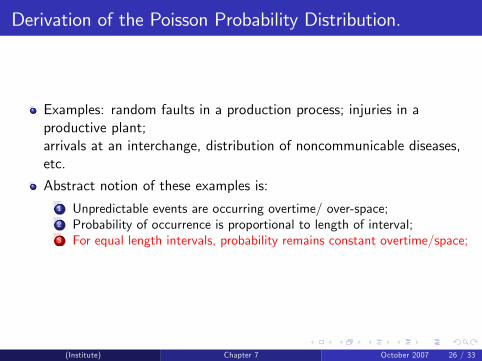
Examples: random faults in a production process; injuries in aproductive plant;arrivals at an interchange, distribution of noncommunicable diseases,etc.
Abstract notion of these examples is:
1 Unpredictable events are occurring overtime/ over-space;2 Probability of occurrence is proportional to length of interval;3 For equal length intervals, probability remains constant overtime/space;4 For a small enough interval, probability of 2+ events is zero.
(Institute) Chapter 7 October 2007 26 / 33
Derivation of the Poisson Probability Distribution.
Examples: random faults in a production process; injuries in aproductive plant;arrivals at an interchange, distribution of noncommunicable diseases,etc.
Abstract notion of these examples is:
1 Unpredictable events are occurring overtime/ over-space;2 Probability of occurrence is proportional to length of interval;3 For equal length intervals, probability remains constant overtime/space;4 For a small enough interval, probability of 2+ events is zero.
(Institute) Chapter 7 October 2007 26 / 33

Derivation of the Poisson Probability Distribution.
Examples: random faults in a production process; injuries in aproductive plant;arrivals at an interchange, distribution of noncommunicable diseases,etc.
Abstract notion of these examples is:1 Unpredictable events are occurring overtime/ over-space;
2 Probability of occurrence is proportional to length of interval;3 For equal length intervals, probability remains constant overtime/space;4 For a small enough interval, probability of 2+ events is zero.
(Institute) Chapter 7 October 2007 26 / 33

Derivation of the Poisson Probability Distribution.
Examples: random faults in a production process; injuries in aproductive plant;arrivals at an interchange, distribution of noncommunicable diseases,etc.
Abstract notion of these examples is:1 Unpredictable events are occurring overtime/ over-space;2 Probability of occurrence is proportional to length of interval;
3 For equal length intervals, probability remains constant overtime/space;4 For a small enough interval, probability of 2+ events is zero.
(Institute) Chapter 7 October 2007 26 / 33
Derivation of the Poisson Probability Distribution.
Examples: random faults in a production process; injuries in aproductive plant;arrivals at an interchange, distribution of noncommunicable diseases,etc.
Abstract notion of these examples is:1 Unpredictable events are occurring overtime/ over-space;2 Probability of occurrence is proportional to length of interval;3 For equal length intervals, probability remains constant overtime/space;
4 For a small enough interval, probability of 2+ events is zero.
(Institute) Chapter 7 October 2007 26 / 33

Derivation of the Poisson Probability Distribution.
Examples: random faults in a production process; injuries in aproductive plant;arrivals at an interchange, distribution of noncommunicable diseases,etc.
Abstract notion of these examples is:1 Unpredictable events are occurring overtime/ over-space;2 Probability of occurrence is proportional to length of interval;3 For equal length intervals, probability remains constant overtime/space;4 For a small enough interval, probability of 2+ events is zero.
(Institute) Chapter 7 October 2007 26 / 33

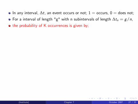
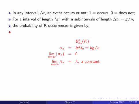
In any interval, ∆t, an event occurs or not; 1 = occurs, 0 = does not;
For a interval of length "g" with n subintervals of length ∆tn = g/n,the probability of K occurrences is given by;
Bnπn (K )
πn = b∆tn = bg/nlimn)∞
(πn) = 0
limn)∞
πn = λ, a constant
λ = bg is a constant determined by the conditions of the experiment.
We consider the distribution given by the limit as n! ∞, butnπn = λ, a constant.
(Institute) Chapter 7 October 2007 27 / 33

In any interval, ∆t, an event occurs or not; 1 = occurs, 0 = does not;For a interval of length "g" with n subintervals of length ∆tn = g/n,
the probability of K occurrences is given by;
Bnπn (K )
πn = b∆tn = bg/nlimn)∞
(πn) = 0
limn)∞
πn = λ, a constant
λ = bg is a constant determined by the conditions of the experiment.
We consider the distribution given by the limit as n! ∞, butnπn = λ, a constant.
(Institute) Chapter 7 October 2007 27 / 33
In any interval, ∆t, an event occurs or not; 1 = occurs, 0 = does not;For a interval of length "g" with n subintervals of length ∆tn = g/n,the probability of K occurrences is given by;
Bnπn (K )
πn = b∆tn = bg/nlimn)∞
(πn) = 0
limn)∞
πn = λ, a constant
λ = bg is a constant determined by the conditions of the experiment.
We consider the distribution given by the limit as n! ∞, butnπn = λ, a constant.
(Institute) Chapter 7 October 2007 27 / 33

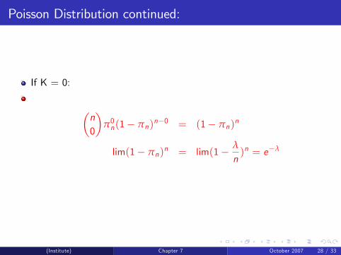
Poisson Distribution continued:
If K = 0:
�n0
�π0n(1� πn)
n�0 = (1� πn)n
lim(1� πn)n = lim(1� λ
n)n = e�λ
(Institute) Chapter 7 October 2007 28 / 33
Poisson Distribution continued:
If K = 0:
�n0
�π0n(1� πn)
n�0 = (1� πn)n
lim(1� πn)n = lim(1� λ
n)n = e�λ
(Institute) Chapter 7 October 2007 28 / 33

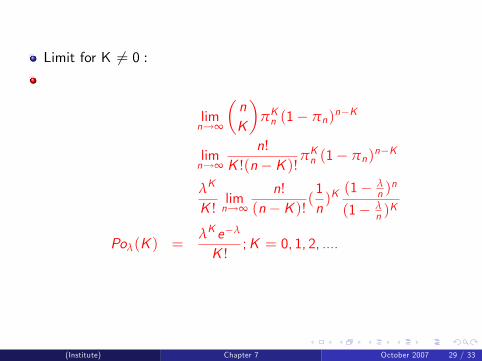
Limit for K 6= 0 :
limn!∞
�nK
�πKn (1� πn)
n�K
limn!∞
n!K !(n�K )! πKn (1� πn)
n�K
λK
K !limn!∞
n!(n�K )! (
1n)K(1� λ
n )n
(1� λn )K
Poλ(K ) =λK e�λ
K !;K = 0, 1, 2, ....
(Institute) Chapter 7 October 2007 29 / 33
Limit for K 6= 0 :
limn!∞
�nK
�πKn (1� πn)
n�K
limn!∞
n!K !(n�K )! πKn (1� πn)
n�K
λK
K !limn!∞
n!(n�K )! (
1n)K(1� λ
n )n
(1� λn )K
Poλ(K ) =λK e�λ
K !;K = 0, 1, 2, ....
(Institute) Chapter 7 October 2007 29 / 33

Poisson Distn. continued
Distribution sums to 1; recall that:
∞
∑k=0
λk
k != 1+ λ+
λ2
2!+
λ3
3!...
= eλ
So that :∞
∑k=0
λk
k !e�λ = 1
(Institute) Chapter 7 October 2007 30 / 33

Poisson Distn. continued
Distribution sums to 1; recall that:
∞
∑k=0
λk
k != 1+ λ+
λ2
2!+
λ3
3!...
= eλ
So that :∞
∑k=0
λk
k !e�λ = 1
(Institute) Chapter 7 October 2007 30 / 33

Theoretical Moments for the Poisson Distn.
Recall the general de�nition for moments about the origin:
µ01(K ) =∞
∑K=0
KλK e�λ
K !
=∞
∑K=1
λK e�λ
(K � 1)!
= λ∞
∑(K�1)=0
λK�1e�λ
(K � 1)! = λ
Similarly, one can show that:
µ2 = λ; µ3 = λ
µ4 = λ+ 3λ2
(Institute) Chapter 7 October 2007 31 / 33

Theoretical Moments for the Poisson Distn.
Recall the general de�nition for moments about the origin:
µ01(K ) =∞
∑K=0
KλK e�λ
K !
=∞
∑K=1
λK e�λ
(K � 1)!
= λ∞
∑(K�1)=0
λK�1e�λ
(K � 1)! = λ
Similarly, one can show that:
µ2 = λ; µ3 = λ
µ4 = λ+ 3λ2
(Institute) Chapter 7 October 2007 31 / 33

Theoretical Moments for the Poisson Distn.
Recall the general de�nition for moments about the origin:
µ01(K ) =∞
∑K=0
KλK e�λ
K !
=∞
∑K=1
λK e�λ
(K � 1)!
= λ∞
∑(K�1)=0
λK�1e�λ
(K � 1)! = λ
Similarly, one can show that:
µ2 = λ; µ3 = λ
µ4 = λ+ 3λ2
(Institute) Chapter 7 October 2007 31 / 33

Theoretical Moments for the Poisson Distn.
Recall the general de�nition for moments about the origin:
µ01(K ) =∞
∑K=0
KλK e�λ
K !
=∞
∑K=1
λK e�λ
(K � 1)!
= λ∞
∑(K�1)=0
λK�1e�λ
(K � 1)! = λ
Similarly, one can show that:
µ2 = λ; µ3 = λ
µ4 = λ+ 3λ2
(Institute) Chapter 7 October 2007 31 / 33

Moments continued, (standardized):
α1 =λ
λ3/2 = λ�1/2
α2 =λ+ 3λ2
λ2= 3+ λ�1
These are the same limits for α1, α2 that hold for the correspondinglimits for the Binomial.
(Institute) Chapter 7 October 2007 32 / 33

Moments continued, (standardized):
α1 =λ
λ3/2 = λ�1/2
α2 =λ+ 3λ2
λ2= 3+ λ�1
These are the same limits for α1, α2 that hold for the correspondinglimits for the Binomial.
(Institute) Chapter 7 October 2007 32 / 33

Conclusion of Chapter 7
(Institute) Chapter 7 October 2007 33 / 33