chapter 6: stability concept of stability - · air parcel expands as it rises air parcel expands...

2/2/2015

1

Chapter 6: Stability

• Concept of Stability• Lapse Rates• How to Use Skew-T Diagram• Determine Stability and Stability Indices

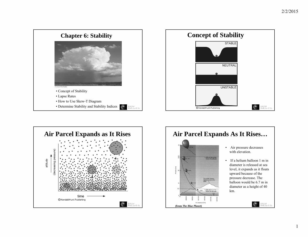
Concept of Stability

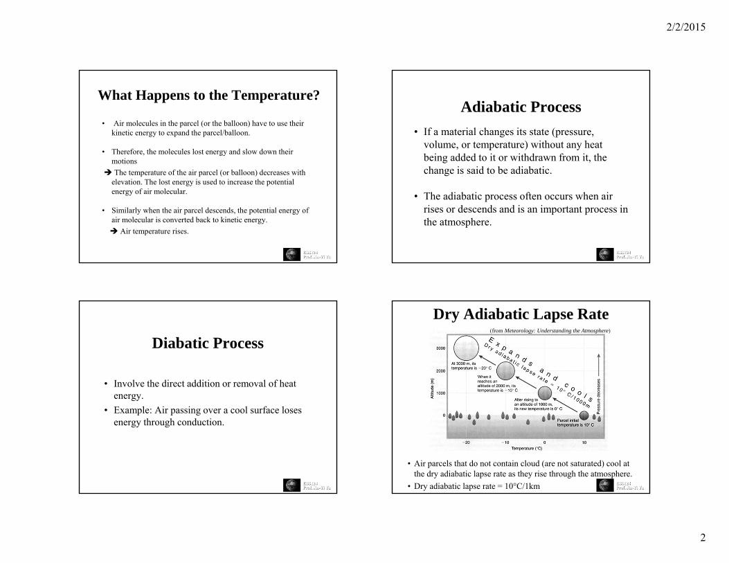
Air Parcel Expands as It Rises Air Parcel Expands As It Rises…

• Air pressure decreases with elevation.

• If a helium balloon 1 m in diameter is released at sea level, it expands as it floats upward because of the pressure decrease. The balloon would be 6.7 m in diameter as a height of 40 km.

(from The Blue Planet)

2/2/2015

2

What Happens to the Temperature?

• Air molecules in the parcel (or the balloon) have to use their kinetic energy to expand the parcel/balloon.

• Therefore, the molecules lost energy and slow down their motions

The temperature of the air parcel (or balloon) decreases with elevation. The lost energy is used to increase the potential energy of air molecular.

• Similarly when the air parcel descends, the potential energy of air molecular is converted back to kinetic energy. Air temperature rises.

Adiabatic Process• If a material changes its state (pressure,

volume, or temperature) without any heat being added to it or withdrawn from it, the change is said to be adiabatic.

• The adiabatic process often occurs when air rises or descends and is an important process in the atmosphere.

• Involve the direct addition or removal of heat energy.

• Example: Air passing over a cool surface loses energy through conduction.

Diabatic Process

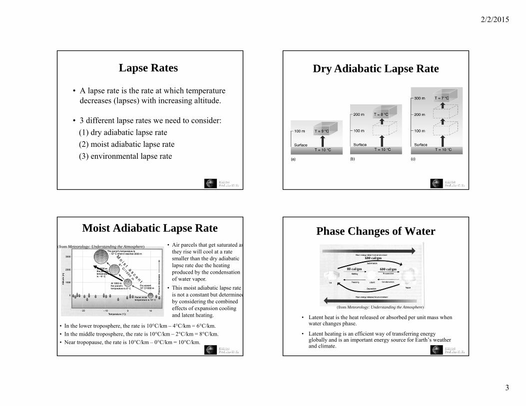
Dry Adiabatic Lapse Rate(from Meteorology: Understanding the Atmosphere)

• Air parcels that do not contain cloud (are not saturated) cool at the dry adiabatic lapse rate as they rise through the atmosphere.

• Dry adiabatic lapse rate = 10°C/1km

2/2/2015

3

Lapse Rates

• A lapse rate is the rate at which temperature decreases (lapses) with increasing altitude.

• 3 different lapse rates we need to consider:(1) dry adiabatic lapse rate(2) moist adiabatic lapse rate(3) environmental lapse rate

Dry Adiabatic Lapse Rate

Moist Adiabatic Lapse Rate(from Meteorology: Understanding the Atmosphere) • Air parcels that get saturated as

they rise will cool at a rate smaller than the dry adiabatic lapse rate due the heating produced by the condensation of water vapor.

• This moist adiabatic lapse rate is not a constant but determinedby considering the combined effects of expansion cooling and latent heating.

• In the lower troposphere, the rate is 10°C/km – 4°C/km = 6°C/km.• In the middle troposphere, the rate is 10°C/km – 2°C/km = 8°C/km.• Near tropopause, the rate is 10°C/km – 0°C/km = 10°C/km.

Phase Changes of Water

• Latent heat is the heat released or absorbed per unit mass when water changes phase.

• Latent heating is an efficient way of transferring energy globally and is an important energy source for Earth’s weather and climate.

(from Meteorology: Understanding the Atmosphere)

80 cal/gm 600 cal/gm

680 cal/gm

2/2/2015

4

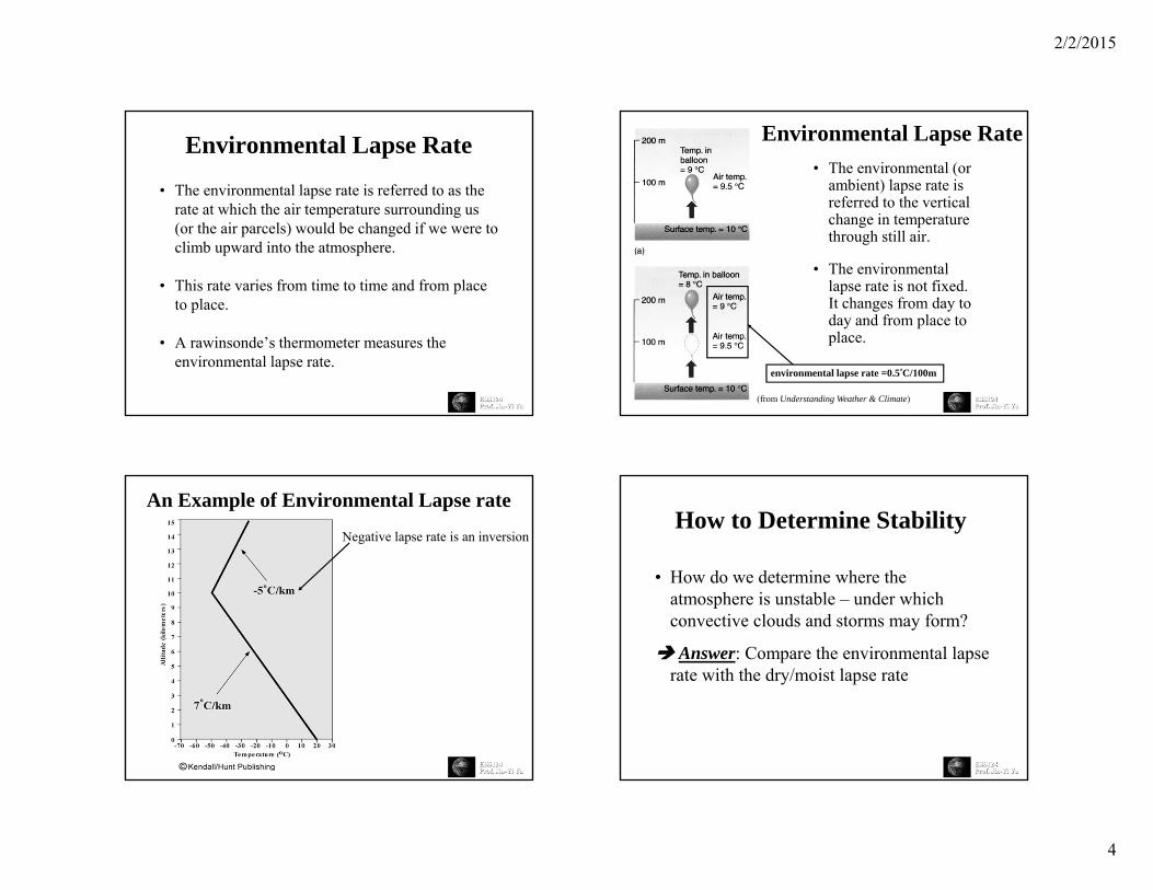
Environmental Lapse Rate

• The environmental lapse rate is referred to as the rate at which the air temperature surrounding us (or the air parcels) would be changed if we were to climb upward into the atmosphere.

• This rate varies from time to time and from place to place.

• A rawinsonde’s thermometer measures the environmental lapse rate.

Environmental Lapse Rate• The environmental (or

ambient) lapse rate is referred to the vertical change in temperature through still air.

• The environmental lapse rate is not fixed. It changes from day to day and from place to place.

environmental lapse rate =0.5°C/100m

(from Understanding Weather & Climate)

An Example of Environmental Lapse rate

Negative lapse rate is an inversionHow to Determine Stability

• How do we determine where the atmosphere is unstable – under which convective clouds and storms may form?

Answer: Compare the environmental lapse rate with the dry/moist lapse rate

2/2/2015

5

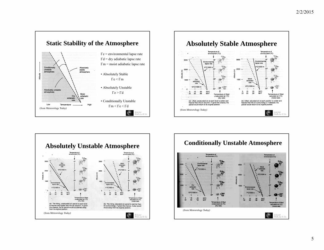
Static Stability of the Atmospheree = environmental lapse rated = dry adiabatic lapse rate m = moist adiabatic lapse rate

• Absolutely Stablee < m

• Absolutely Unstablee > d

• Conditionally Unstablem < e < d

(from Meteorology Today)

Absolutely Stable Atmosphere


Absolutely Unstable Atmosphere


Conditionally Unstable Atmosphere


2/2/2015

6

ESS124Prof. Jin-Yi Yu

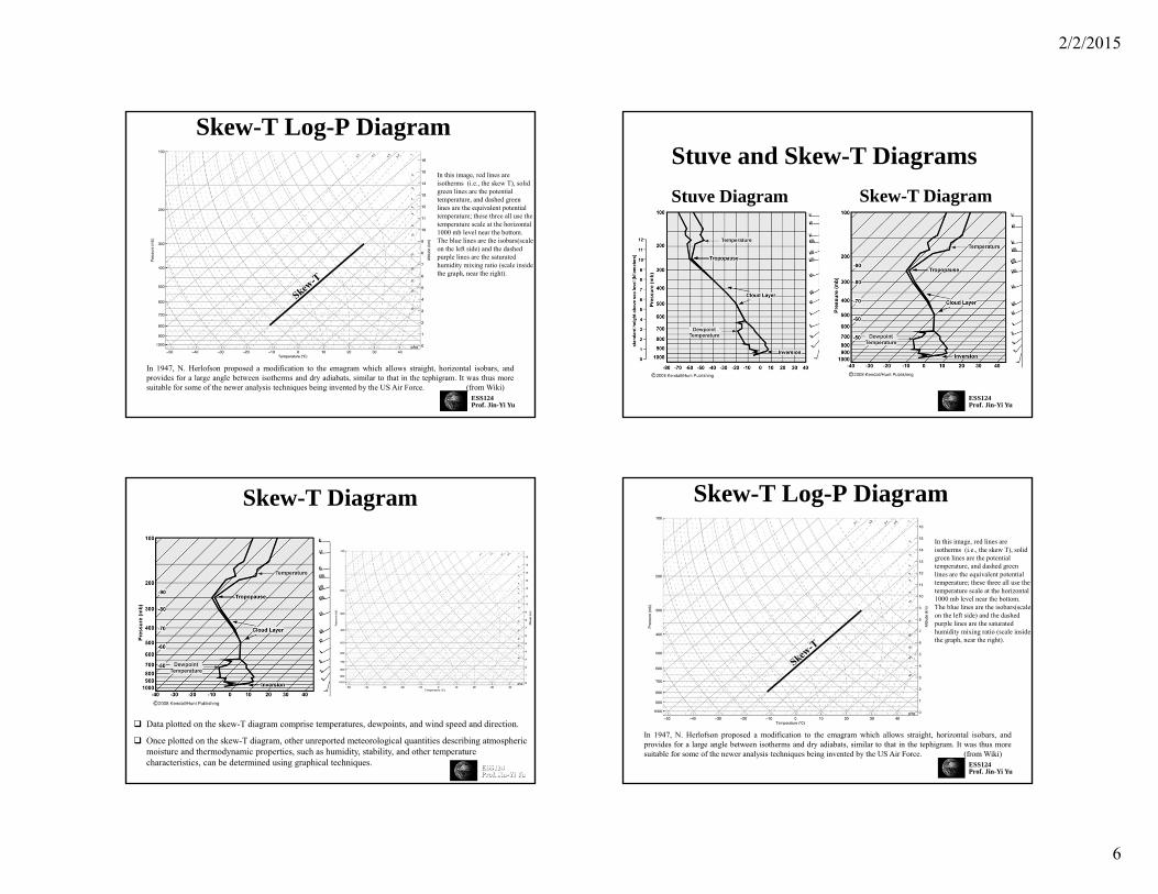
Skew-T Log-P Diagram

In 1947, N. Herlofson proposed a modification to the emagram which allows straight, horizontal isobars, andprovides for a large angle between isotherms and dry adiabats, similar to that in the tephigram. It was thus moresuitable for some of the newer analysis techniques being invented by the US Air Force. (from Wiki)

In this image, red lines are isotherms (i.e., the skew T), solid green lines are the potential temperature, and dashed green lines are the equivalent potential temperature; these three all use the temperature scale at the horizontal 1000 mb level near the bottom. The blue lines are the isobars(scale on the left side) and the dashed purple lines are the saturated humidity mixing ratio (scale inside the graph, near the right).


Stuve and Skew-T DiagramsStuve Diagram Skew-T Diagram

Data plotted on the skew-T diagram comprise temperatures, dewpoints, and wind speed and direction.

Once plotted on the skew-T diagram, other unreported meteorological quantities describing atmospheric moisture and thermodynamic properties, such as humidity, stability, and other temperature characteristics, can be determined using graphical techniques.

Skew-T Diagram


Skew-T Log-P Diagram

In 1947, N. Herlofson proposed a modification to the emagram which allows straight, horizontal isobars, andprovides for a large angle between isotherms and dry adiabats, similar to that in the tephigram. It was thus moresuitable for some of the newer analysis techniques being invented by the US Air Force. (from Wiki)

In this image, red lines are isotherms (i.e., the skew T), solid green lines are the potential temperature, and dashed green lines are the equivalent potential temperature; these three all use the temperature scale at the horizontal 1000 mb level near the bottom. The blue lines are the isobars(scale on the left side) and the dashed purple lines are the saturated humidity mixing ratio (scale inside the graph, near the right).

2/2/2015

7


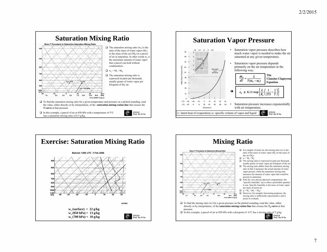
Saturation Mixing Ratio The saturation mixing ratio (ws) is the

ratio of the mass of water vapor (Mv) to the mass of dry air (Md) in a parcel of air at saturation. In other words ws is the maximum amount of water vapor that a parcel can hold without condensation.

ws = Mv / Md

The saturation mixing ratio is expressed in parts per thousand, usually grams of water vapor per kilogram of dry air.

To find the saturation mixing ratio for a given temperature and pressure on a plotted sounding, read the value, either directly or by interpolation, of the saturation mixing-ration line that crosses the T curve at that pressure.

In this example, a parcel of air at 850 hPa with a temperature of 5°C has a saturation mixing ratio of 6.5 g/kg.


Saturation Vapor Pressure• Saturation vapor pressure describes how

much water vapor is needed to make the air saturated at any given temperature.

• Saturation vapor pressure depends primarily on the air temperature in the following way:

• Saturation pressure increases exponentially with air temperature.

TheClausius-ClapeyronEquation

L: latent heat of evaporation; : specific volume of vapor and liquid


Exercise: Saturation Mixing Ratio

ws (surface) = 22 g/kg ws (850 hPa) = 13 g/kg ws (700 hPa) = 10 g/kg ESS124

Prof. Jin-Yi Yu

Mixing Ratio In a sample of moist air, the mixing ratio (w) is the

ratio of the mass of water vapor (Mv) to the mass of dry air (Md):

w = Mv / Md The mixing ratio is expressed in parts per thousand,

usually grams of water vapor per kilogram of dry air. The mixing ratio differs from the saturation mixing

ratio in that it measures the actual amount of water vapor present, while the saturation mixing ratio measures the amount of water vapor that would be present at saturation.

Note for very precise physical computations, the "specific humidity" (q) is often a preferable quantity to use. Specific humidity is the mass of water vapor per mass of moist air:

q = Mv / (Mv + Md) However, for synoptic forecasting purposes, the

mixing ratio is sufficiently representative and is easier to evaluate.

To find the mixing ratio (w) for a given pressure on the plotted sounding, read the value, either directly or by interpolation, of the saturation mixing-ration line that crosses the Td curve at that pressure.

In this example, a parcel of air at 850 hPa with a dewpoint of -6°C has a mixing ratio of 3 g/kg.

2/2/2015

8


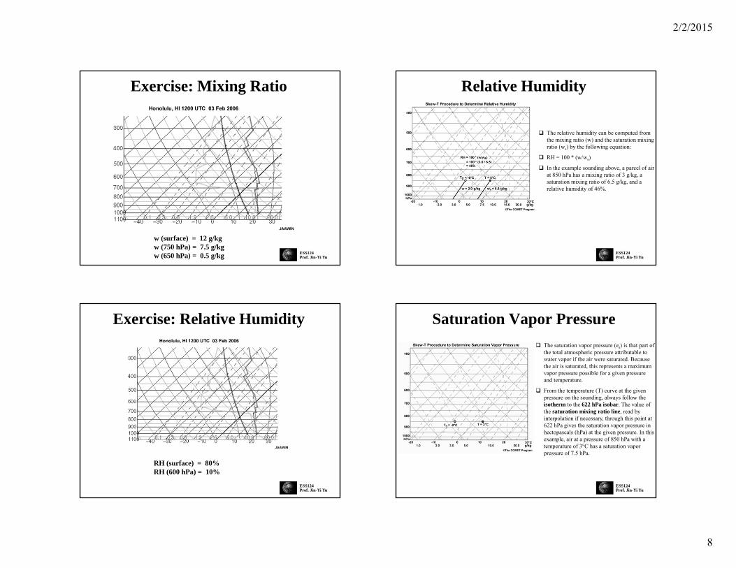
Exercise: Mixing Ratio

w (surface) = 12 g/kg w (750 hPa) = 7.5 g/kg w (650 hPa) = 0.5 g/kg ESS124

Prof. Jin-Yi Yu

Relative Humidity

The relative humidity can be computed from the mixing ratio (w) and the saturation mixing ratio (ws) by the following equation:

RH = 100 * (w/ws)

In the example sounding above, a parcel of air at 850 hPa has a mixing ratio of 3 g/kg, a saturation mixing ratio of 6.5 g/kg, and a relative humidity of 46%.


Exercise: Relative Humidity

RH (surface) = 80%RH (600 hPa) = 10%


Saturation Vapor Pressure The saturation vapor pressure (es) is that part of

the total atmospheric pressure attributable to water vapor if the air were saturated. Because the air is saturated, this represents a maximum vapor pressure possible for a given pressure and temperature.

From the temperature (T) curve at the given pressure on the sounding, always follow the isotherm to the 622 hPa isobar. The value of the saturation mixing ratio line, read by interpolation if necessary, through this point at 622 hPa gives the saturation vapor pressure in hectopascals (hPa) at the given pressure. In this example, air at a pressure of 850 hPa with a temperature of 3°C has a saturation vapor pressure of 7.5 hPa.

2/2/2015

9


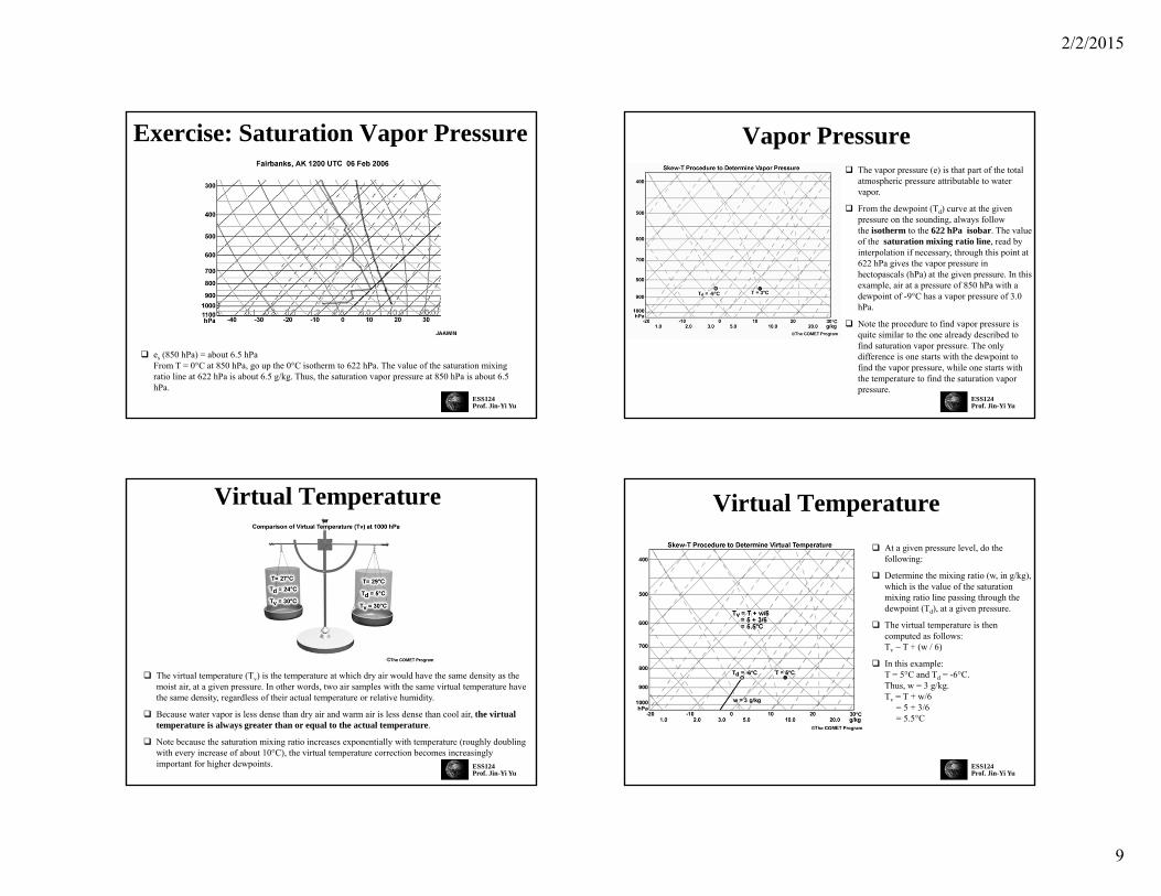
Exercise: Saturation Vapor Pressure

es (850 hPa) = about 6.5 hPaFrom T = 0°C at 850 hPa, go up the 0°C isotherm to 622 hPa. The value of the saturation mixing ratio line at 622 hPa is about 6.5 g/kg. Thus, the saturation vapor pressure at 850 hPa is about 6.5 hPa.


Vapor Pressure The vapor pressure (e) is that part of the total

atmospheric pressure attributable to water vapor.

From the dewpoint (Td) curve at the given pressure on the sounding, always follow the isotherm to the 622 hPa isobar. The value of the saturation mixing ratio line, read by interpolation if necessary, through this point at 622 hPa gives the vapor pressure in hectopascals (hPa) at the given pressure. In this example, air at a pressure of 850 hPa with a dewpoint of -9°C has a vapor pressure of 3.0 hPa.

Note the procedure to find vapor pressure is quite similar to the one already described to find saturation vapor pressure. The only difference is one starts with the dewpoint to find the vapor pressure, while one starts with the temperature to find the saturation vapor pressure.


Virtual Temperature

The virtual temperature (Tv) is the temperature at which dry air would have the same density as the moist air, at a given pressure. In other words, two air samples with the same virtual temperature have the same density, regardless of their actual temperature or relative humidity.

Because water vapor is less dense than dry air and warm air is less dense than cool air, the virtual temperature is always greater than or equal to the actual temperature.

Note because the saturation mixing ratio increases exponentially with temperature (roughly doubling with every increase of about 10°C), the virtual temperature correction becomes increasingly important for higher dewpoints. ESS124

Prof. Jin-Yi Yu

Virtual Temperature At a given pressure level, do the

following:

Determine the mixing ratio (w, in g/kg), which is the value of the saturation mixing ratio line passing through the dewpoint (Td), at a given pressure.

The virtual temperature is then computed as follows:Tv ~ T + (w / 6)

In this example:T = 5°C and Td = -6°C.Thus, w = 3 g/kg.Tv = T + w/6

= 5 + 3/6= 5.5°C

2/2/2015

10


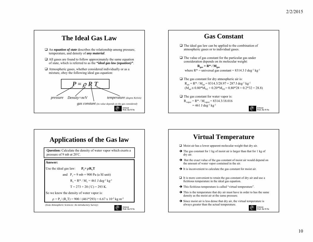
The Ideal Gas Law An equation of state describes the relationship among pressure,

temperature, and density of any material.

All gases are found to follow approximately the same equation of state, which is referred to as the “ideal gas law (equation)”.

Atmospheric gases, whether considered individually or as a mixture, obey the following ideal gas equation:

P = R T

pressure Density=m/V temperature (degree Kelvin)

gas constant (its value depends on the gas considered)ESS124Prof. Jin-Yi Yu

Gas Constant The ideal gas law can be applied to the combination of

atmospheric gases or to individual gases.

The value of gas constant for the particular gas under consideration depends on its molecular weight:

Rgas = R* / Mgas where R* = universal gas constant = 8314.3 J deg-1 kg-1

The gas constant for dry atmospheric air is:Rair = R* / Mair = 8314.3/28.97 = 287 J deg-1 kg-1

(Mair 0.80*MN2 + 0.20*MO2 = 0.80*28 + 0.2*32 = 28.8)

The gas constant for water vapor is: Rvapor = R* / Mvapor = 8314.3/18.016

= 461 J deg-1 kg-1


Applications of the Gas lawQuestion: Calculate the density of water vapor which exerts a pressure of 9 mb at 20°C.

Answer:

Use the ideal gas law: Pv= RvT

and Pv = 9 mb = 900 Pa (a SI unit)

Rv = R* / Mv = 461 J deg-1 kg-1

T = 273 + 20 (°C) = 293 K.

So we know the density of water vapor is:

= Pv/ (RvT) = 900 / (461*293) = 6.67 x 10-3 kg m-3

(from Atmospheric Sciences: An introductory Survey)ESS124Prof. Jin-Yi Yu

Virtual Temperature Moist air has a lower apparent molecular weight that dry air.

The gas constant for 1 kg of moist air is larger than that for 1 kg of dry air.

But the exact value of the gas constant of moist air would depend on the amount of water vapor contained in the air.

It is inconvenient to calculate the gas constant for moist air.

It is more convenient to retain the gas constant of dry air and use a fictitious temperature in the ideal gas equation.

This fictitious temperature is called “virtual temperature”.

This is the temperature that dry air must have in order to has the same density as the moist air at the same pressure.

Since moist air is less dense that dry air, the virtual temperature is always greater than the actual temperature.

2/2/2015

11


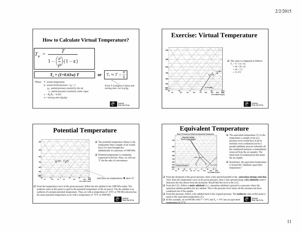
How to Calculate Virtual Temperature?

Where T: actual temperaturep: actual (total) pressure = pd + e

pd: partial pressure exerted by dry aire: partial pressure exerted by water vapor

= Rd/Rv = 0.622w = mixing ratio (kg/kg)

Tv = (1+0.61w) T or

If use T in degrees Celsius and mixing ratio (w) in g/kg


Exercise: Virtual Temperature

The value is computed as follows:Tv = T + (w / 6)

= 10 + (8 / 6)= 10 + 1.3= 11.3°C


Potential Temperature The potential temperature (theta) is the

temperature that a sample of air would have if it were brought dry-adiabatically to a pressure of 1000 hPa.

Potential temperature is commonly expressed in kelvins. Here, we will use °C for the sake of convenience.

From the temperature curve at the given pressure, follow the dry adiabat to the 1000 hPa isobar. The isotherm value at this point is equal to the potential temperature of the air parcel. The dry adiabat is an isotherm of constant potential temperature. Thus, air with a temperature of -10°C at 700 hPa (shown) has the same potential temperature as air with a temperature of 19°C at 1000 hPa.

(red lines are temperatures skew-T)


Equivalent Temperature The equivalent temperature (Te) is the

temperature a sample of air at a pressure level would have if all its moisture were condensed out by a pseudo-adiabatic process (whereby all the condensed moisture is immediately removed from the air sample). The latent heat of condensation then heats the air sample.

Sometimes, the equivalent temperature is termed the "adiabatic equivalent temperature."

From the dewpoint at the given pressure, draw a line upward parallel to the saturation mixing ratio line. Also, from the temperature curve at the given pressure, draw a line upward along a dry adiabatic until it intersects the line drawn from the dewpoint. Recall that this level is the LCL.

From the LCL, follow a moist adiabatic (i.e., saturation adiabatic) upward to a pressure where the saturation adiabat parallels the dry adiabat. This is the pressure level where all the moisture has been condensed out of the sample.

From this pressure, follow a dry adiabat back to the original pressure. The isotherm value at this point is equal to the equivalent temperature (Te).

In this example, air at 850 hPa with T = 10°C and Td = -8°C has an equivalent temperature of 17°C.

2/2/2015

12


Exercise: Equivalent Temperature

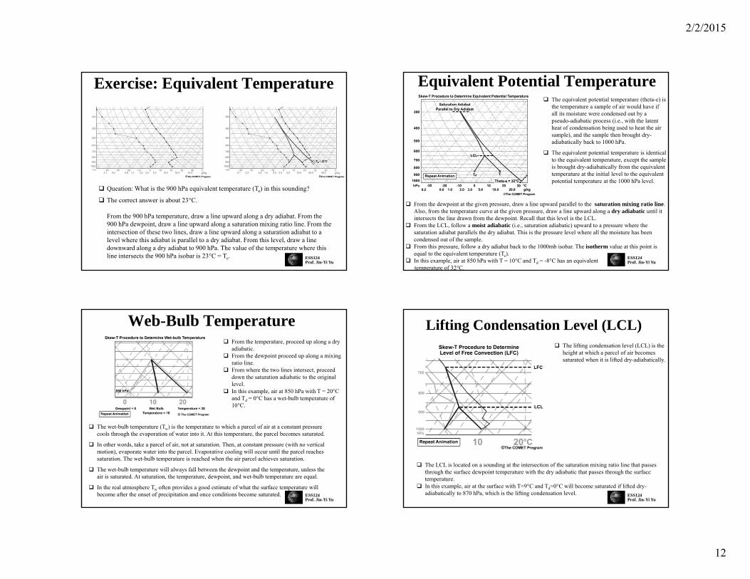
Queation: What is the 900 hPa equivalent temperature (Te) in this sounding?

The correct answer is about 23°C.

From the 900 hPa temperature, draw a line upward along a dry adiabat. From the 900 hPa dewpoint, draw a line upward along a saturation mixing ratio line. From the intersection of these two lines, draw a line upward along a saturation adiabat to a level where this adiabat is parallel to a dry adiabat. From this level, draw a line downward along a dry adiabat to 900 hPa. The value of the temperature where this line intersects the 900 hPa isobar is 23°C = Te. ESS124

Prof. Jin-Yi Yu

Equivalent Potential Temperature The equivalent potential temperature (theta-e) is

the temperature a sample of air would have if all its moisture were condensed out by a pseudo-adiabatic process (i.e., with the latent heat of condensation being used to heat the air sample), and the sample then brought dry-adiabatically back to 1000 hPa.

The equivalent potential temperature is identical to the equivalent temperature, except the sample is brought dry-adiabatically from the equivalent temperature at the initial level to the equivalent potential temperature at the 1000 hPa level.

From the dewpoint at the given pressure, draw a line upward parallel to the saturation mixing ratio line. Also, from the temperature curve at the given pressure, draw a line upward along a dry adiabatic until it intersects the line drawn from the dewpoint. Recall that this level is the LCL.

From the LCL, follow a moist adiabatic (i.e., saturation adiabatic) upward to a pressure where the saturation adiabat parallels the dry adiabat. This is the pressure level where all the moisture has been condensed out of the sample.

From this pressure, follow a dry adiabat back to the 1000mb isobar. The isotherm value at this point is equal to the equivalent temperature (Te).

In this example, air at 850 hPa with T = 10°C and Td = -8°C has an equivalent temperature of 32°C.


Web-Bulb Temperature

The wet-bulb temperature (Tw) is the temperature to which a parcel of air at a constant pressure cools through the evaporation of water into it. At this temperature, the parcel becomes saturated.

In other words, take a parcel of air, not at saturation. Then, at constant pressure (with no vertical motion), evaporate water into the parcel. Evaporative cooling will occur until the parcel reaches saturation. The wet-bulb temperature is reached when the air parcel achieves saturation.

The wet-bulb temperature will always fall between the dewpoint and the temperature, unless the air is saturated. At saturation, the temperature, dewpoint, and wet-bulb temperature are equal.

In the real atmosphere Tw often provides a good estimate of what the surface temperature will become after the onset of precipitation and once conditions become saturated.

From the temperature, proceed up along a dry adiabatic.

From the dewpoint proceed up along a mixing ratio line.

From where the two lines intersect, proceed down the saturation adiabatic to the original level.

In this example, air at 850 hPa with T = 20°C and Td = 0°C has a wet-bulb temperature of 10°C.


Lifting Condensation Level (LCL) The lifting condensation level (LCL) is the

height at which a parcel of air becomes saturated when it is lifted dry-adiabatically.

The LCL is located on a sounding at the intersection of the saturation mixing ratio line that passes through the surface dewpoint temperature with the dry adiabatic that passes through the surface temperature.

In this example, air at the surface with T=9°C and Td=0°C will become saturated if lifted dry-adiabatically to 870 hPa, which is the lifting condensation level.

2/2/2015

13


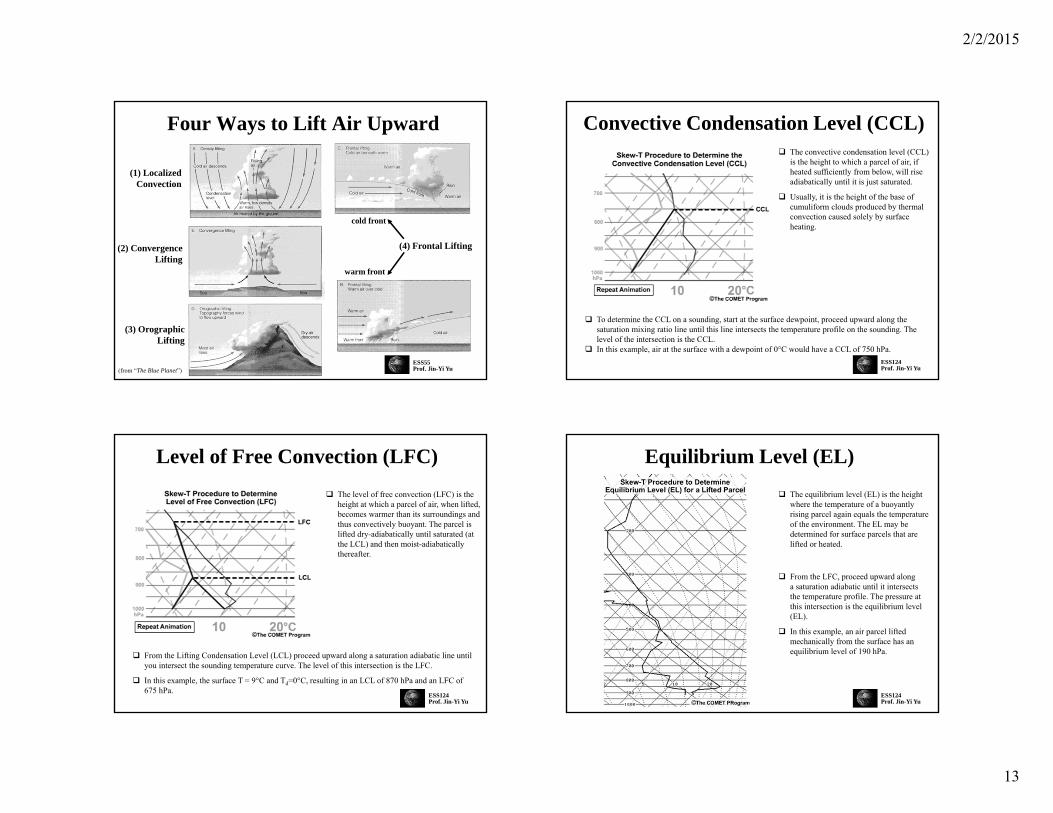
Four Ways to Lift Air Upward

(1) LocalizedConvection

(2) ConvergenceLifting

(3) OrographicLifting

(4) Frontal Lifting

warm front

cold front

(from “The Blue Planet”)ESS124Prof. Jin-Yi Yu

Convective Condensation Level (CCL) The convective condensation level (CCL)

is the height to which a parcel of air, if heated sufficiently from below, will rise adiabatically until it is just saturated.

Usually, it is the height of the base of cumuliform clouds produced by thermal convection caused solely by surface heating.

To determine the CCL on a sounding, start at the surface dewpoint, proceed upward along the saturation mixing ratio line until this line intersects the temperature profile on the sounding. The level of the intersection is the CCL.

In this example, air at the surface with a dewpoint of 0°C would have a CCL of 750 hPa.


Level of Free Convection (LFC) The level of free convection (LFC) is the

height at which a parcel of air, when lifted, becomes warmer than its surroundings and thus convectively buoyant. The parcel is lifted dry-adiabatically until saturated (at the LCL) and then moist-adiabatically thereafter.

From the Lifting Condensation Level (LCL) proceed upward along a saturation adiabatic line until you intersect the sounding temperature curve. The level of this intersection is the LFC.

In this example, the surface T = 9°C and Td=0°C, resulting in an LCL of 870 hPa and an LFC of 675 hPa.


Equilibrium Level (EL) The equilibrium level (EL) is the height

where the temperature of a buoyantly rising parcel again equals the temperature of the environment. The EL may be determined for surface parcels that are lifted or heated.

From the LFC, proceed upward along a saturation adiabatic until it intersects the temperature profile. The pressure at this intersection is the equilibrium level (EL).

In this example, an air parcel lifted mechanically from the surface has an equilibrium level of 190 hPa.

2/2/2015

14


Maximum Parcel Level (MPL)

The maximum parcel level (MPL) is the level to which a parcel will travel before exhausting all of its upward momentum.

When a parcel travels through the equilibrium level (EL), its upward acceleration ceases as it becomes colder than its surroundings, but its upward momentum continues to propel the parcel to a higher level.

Therefore, the MPL is always at a higher level than the equilibrium level. Practically speaking, the MPL is the maximum predicted height of a thunderstorm for a given sounding.


Determining Maximum Parcel Level (MPL)

First, determine the equilibrium level (EL) for either a lifted or heated parcel, whichever is most appropriate for the situation.

Then continue upward along a saturation adiabatic until the negative area above the EL is equal to the positive area (CAPE) below the EL.

For computer-generated skew-Ts, the MPL is usually computed automatically.


Determining Maximum Parcel Level (MPL)

First, determine the equilibrium level (EL) for either a lifted or heated parcel, whichever is most appropriate for the situation.

Then continue upward along a saturation adiabatic until the negative area above the EL is equal to the positive area (CAPE) below the EL.

For computer-generated skew-Ts, the MPL is usually computed automatically.

Stability Indices(1) Environmental Lapse rate(2) Lifted Index = T (environment at 500mb) – T (parcel lifted to 500mb)(3) Showalter Index: similar to lifted index but was lifted to 850mb(4) CAPE (Convective Available Potential Energy): derived from soundings(5) Convective INHibition (CINH) Index(6) K Index(7) Total Totals Index(8) SWEAT (Severe Weather Threat) Index

2/2/2015

15


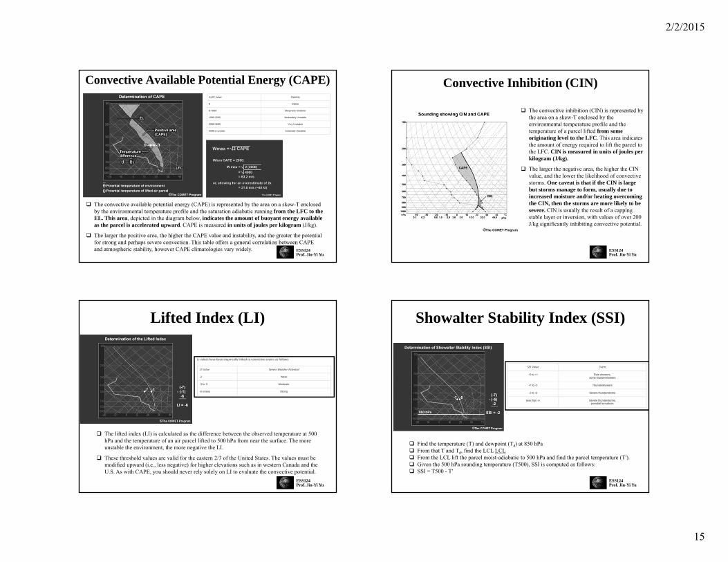
Convective Available Potential Energy (CAPE)

The convective available potential energy (CAPE) is represented by the area on a skew-T enclosed by the environmental temperature profile and the saturation adiabatic running from the LFC to the EL. This area, depicted in the diagram below, indicates the amount of buoyant energy available as the parcel is accelerated upward. CAPE is measured in units of joules per kilogram (J/kg).

The larger the positive area, the higher the CAPE value and instability, and the greater the potential for strong and perhaps severe convection. This table offers a general correlation between CAPE and atmospheric stability, however CAPE climatologies vary widely. ESS124

Prof. Jin-Yi Yu

Convective Inhibition (CIN)

The convective inhibition (CIN) is represented by the area on a skew-T enclosed by the environmental temperature profile and the temperature of a parcel lifted from some originating level to the LFC. This area indicates the amount of energy required to lift the parcel to the LFC. CIN is measured in units of joules per kilogram (J/kg).

The larger the negative area, the higher the CIN value, and the lower the likelihood of convective storms. One caveat is that if the CIN is large but storms manage to form, usually due to increased moisture and/or heating overcoming the CIN, then the storms are more likely to be severe. CIN is usually the result of a capping stable layer or inversion, with values of over 200 J/kg significantly inhibiting convective potential.


Lifted Index (LI)

The lifted index (LI) is calculated as the difference between the observed temperature at 500 hPa and the temperature of an air parcel lifted to 500 hPa from near the surface. The more unstable the environment, the more negative the LI.

These threshold values are valid for the eastern 2/3 of the United States. The values must be modified upward (i.e., less negative) for higher elevations such as in western Canada and the U.S. As with CAPE, you should never rely solely on LI to evaluate the convective potential.


Showalter Stability Index (SSI)

Find the temperature (T) and dewpoint (Td) at 850 hPa From that T and Td, find the LCL LCL From the LCL lift the parcel moist-adiabatic to 500 hPa and find the parcel temperature (T′). Given the 500 hPa sounding temperature (T500), SSI is computed as follows: SSI = T500 - T′

2/2/2015

16


K Index (KI)

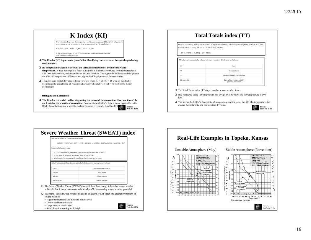
The K index (KI) is particularly useful for identifying convective and heavy-rain-producing environments.

Its computation takes into account the vertical distribution of both moisture and temperature. It does not require a skew-T diagram; it is simply computed from temperatures at 850, 700, and 500 hPa, and dewpoints at 850 and 700 hPa. The higher the moisture and the greater the 850-500 temperature difference, the higher the KI and potential for convection.

Thunderstorm probability ranges from very low when KI < 20 (KI < 15 west of the Rocky Mountains) to a likelihood of widespread activity when KI > 35 (KI > 30 west of the Rocky Mountains).

Strengths and Limitations

The K index is a useful tool for diagnosing the potential for convection. However, it can't be used to infer the severity of convection. Because it uses 850 hPa data, it is not applicable in the Rocky Mountain region, where the surface pressure is typically less than 850 hPa. ESS124

Prof. Jin-Yi Yu

Total Totals index (TT)

The Total Totals index (TT) is yet another severe weather index.

It is computed using the temperature and dewpoint at 850 hPa and the temperature at 500 hPa.

The higher the 850 hPa dewpoint and temperature and the lower the 500 hPa temperature, the greater the instability and the resulting TT value.


Severe Weather Threat (SWEAT) index

The Severe Weather Threat (SWEAT) index differs from many of the other severe weather indices in that it takes into account the wind profile in assessing severe weather potential.

In general, the following conditions lead to a higher SWEAT index and greater probability of severe weather:• Higher temperature and moisture at low levels• Cooler temperatures aloft• Large vertical wind shear• Wind direction veering with height

Real-Life Examples in Topeka, Kansas

Unstable Atmosphere (May) Stable Atmosphere (November)

2/2/2015

17

An Example How Thunderstorm Forms?

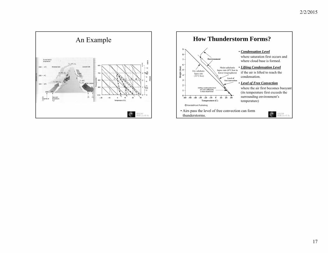
• Condensation Levelwhere saturation first occurs and where cloud base is formed.

• Lifting Condensation Levelif the air is lifted to reach the condensation.

• Level of Free Convectionwhere the air first becomes buoyant (its temperature first exceeds the surrounding environment’s temperature)

• Airs pass the level of free convection can form thunderstorms.

chapter 6: stability concept of stability - · air parcel expands as it rises air parcel expands...

Documents