chapter 6 simulated annealing algorithm -...
TRANSCRIPT
82
CHAPTER 6
SIMULATED ANNEALING ALGORITHM
SAA has broad appeal in many areas and has attractive and unique
features when compared with others. The key feature of SAA is that it
provides a means to escape local optima by allowing hill-climbing moves.
This chapter discusses the SAA based heuristic as a proposed solution
methodology to solve the multi-period fixed charge models proposed in this
thesis.
6.1 INTRODUCTION
There are many research works in the field of Operations Research
using SAA heuristic. Eglese (1990) described the SAA and the physical
analogy on which it is based. Some significant theoretical results are
presented before describing how the algorithm may be implemented and some
of the choices facing the user of this method. An overview of SAA
experiments is given some suggestions are made for ways to improve the
performance of the algorithm by modifying the �pure� SAA approach. Pirlot
(1996) presented a tutorial introduction to three recent yet widely used
general heuristics: Simulated Annealing, Tabu Search, and Genetic
Algorithms. A relatively precise description and an example of application are
provided for each of the methods, as well as a tentative evaluation and
comparison from a pragmatic point of view. Ponnambalam et al (1999)
proposed a SAA for the job shop scheduling problem with the objective of
minimization of makespan time. They compared the proposed SAA with
83
existing genetic algorithms and the presented the comparative results. For
comparative evaluation, they used a wide variety of data sets. They found that
the proposed algorithm performed well for scheduling in the job shop.
Jayaraman and Ross (2003) addressed a class of distribution network design
problems, which is characterized by multiple product families, a central
manufacturing plant site, multiple distribution centre and cross-docking sites,
and retail outlets (customer zones) which demand multiple units of several
commodities. They proposed SAA for the class of distribution network
problems to generate globally feasible, near optimal distribution system
design and utilization strategies. Ji et al (2006) proposed an improved
simulated annealing (ISA), a global optimization algorithm for solving the
linear constrained optimization problems, of which the main characteristics
are that only one component of current solution is changed based on the
Gaussian distribution and ISA can directly solve the linear constrained
optimization problems. They solved 6 benchmark functions with the lower
and upper bounds constraints and 6 functions with linear constraints, and
proved that ISA is superior to the classical techniques for solving the
problems with lower and upper bounds. Lim et al (2006) proposed a
simulated annealing with hill climbing algorithm for the Traveling
Tournament Problem (TTP). They adapted the approach for TTP by
parallelizing components which search for better timetables and better team
assignments, instead of using these sequentially. Experiments have showed
that the hybrid approach gives results which are comparable to or better than
the best solutions for benchmark sets. Mansouri (2006) proposed a multi-
objective simulated annealing (MOSA) solution approach to a bi-criteria
sequencing problem to coordinate required set-ups between two successive
stages of a supply chain in a flow shop pattern. Each production batch has two
distinct attributes and a set-up occurs in each stage when the corresponding
attribute of the two successive batches are different. There are two objectives
including: minimizing total set-ups and minimizing the maximum number of
84
set-ups between the two stages that are both NP-hard problems. They
evaluated the Performance of the proposed MOSA using true Pareto-optimal
solutions of small problems found via total enumeration. They also compared
the MOSA against a lower bound in large problems. Comparative
experiments showed that the MOSA is robust in finding true Pareto-optimal
solutions in small problems.
The summary of the SAA applications is as follows:
� SAA is a proven tool for many hard optimization problems,
and if implemented well, often produces good results in a
short runtime.
� SAA configuration decisions proceed in a logical manner.
Hence it is simple to formulate and handle mixed, discrete
and continuous problem with ease.
� Its solution does not get trapped in a local minimum or
maximum by sometimes accepting even the inferior move.
� The methodology of SAA has broad appeal in many areas
(Balram Suman 2004) and has attractive and unique features
when compared with other optimization techniques (Suman
and Kumar 2006).
� On the above considerations, the four multi-period fixed
charge models have been solved using SAA based heuristic to
find the optimal or near optimal solutions in a reasonable
computational time.
85
6.2 FUNDAMENTALS OF SAA
The algorithm was first proposed by Kirkpatrick et al (1983) based
on the physical annealing process of solids. First, the solid is heated up to a
high temperature. At that temperature all the molecules of the material have
high energies and randomly arrange themselves into a liquid state. Then the
temperature decreases at a certain rate which will reduce the molecules�
energies and their freedom to arrange them. Finally, the temperature goes
down to such a level that all the molecules lose their freedom to arrange
themselves then the material crystallizes. If the temperature decreases at a
proper rate, the material can obtain a regular internal structure at the minimum
energy state. However, if the temperature goes down too fast, the
irregularities and defects will appear in the solid and the system will be at a
local minimum energy state. In analogy to the annealing process, the feasible
solutions of the optimization problem are correspond to the states of the
material, the objective function values computed at these solutions are
represented by the energies of the states, the optimal solution to the problem
can be viewed as the minimum energy state of the material and the
suboptimal solutions correspond to the local minimum energy states. Similar
to most classes of meta-heuristics that are based on gradual �local
improvements�, SAA starts off with a non-optimal initial configuration
(which may be random) and at high temperatureTE . A new configuration is
created by using a suitable mechanism with reference to the initial
configuration and calculating the corresponding cost differential ( Delta ). If
the cost is reduced, then the new configuration is accepted, otherwise that is
accepted with a probability exp (- Delta /TE ) and the process is repeated
until a termination criterion is met. The general structure of the SAA is as
shown below.
86
Step 1: Get an initial solution iS , randomly
Step 2: Set an initial temperature, 0�TE
Step 3: While not frozen do the following:
Step 3.1: Do the following n times:
Step 3.1.1: Sample a neighbour Si1 from Si
Step 3.1.2: Let Delta= cost (Si1) � cost (Si)
Step 3.1.3: If Delta< 0 then ( i.e. downhill move) set Si = Si1 else ( i.e.
uphill move) set Si = Si1 with the probability of exp (-Delta/TE )
Step 3.2: Set TE=TE*�, where � is the reduction factor
Step 4: Return Si
6.3 PROPOSED SAA
Multi-period fixed charge problems using SAA requires a separate
string coding and decoding procedural steps for each and every period. After
deriving the best distribution schedule for each period, they have to be
integrated for overall minimum cost. This difficulty is not present while
solving single-period problem using SAA because it requires only a single
integrated string for coding and decoding procedural steps. Moreover this
single-period formulation can be used while solving the multi-period
distribution problem in a multi-stage supply chain environment. Hence the
proposed SAA based heuristic is structured to solve the multi-period fixed
charge problems in two stages as stage-I and stage-II. Stage-I accepts the data
of multi-period fixed charge problem as input and transforms them as a single
period data set. Stage-II is the application of SAA that evolves the best
distribution schedule to the multi-period fixed charge problem with the
87
modulated data. The following sections delineate the proposed SAA with a
numerical example of multi-period fixed charge problems.
In the proposed SAA, the solution is represented as a gene type
representation of a feasible solution in the form of a finite length array called
string. The string is the permutation of cell numbers of a modulated single
period distribution matrix. Each cell in the distribution matrix known as gene
is identified with a unique number that assume discrete allocation values
pertaining to the problem's solution. The first gene in the string provides
location identification in the single-period matrix where the first allotment is
made by the minimum value of either supply (row) or demand (column). The
same procedure is followed until the whole single-period matrix is filled by
distribution allotments. Moreover, the string is structured as two parts. The
first part is framed by the cell numbers of prompt deliveries of the distribution
matrix and the second part is framed by the remaining cell numbers of the
distribution matrix. In order to maintain feasibility, the changes are made
separately in the two parts of the string.
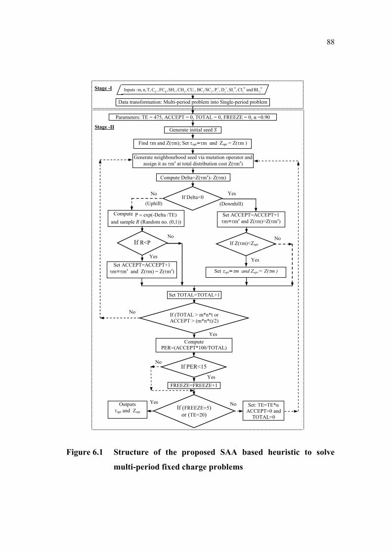
The framework of the proposed SAA based heuristic (coded in
Turbo C++) is shown in Figure 6.1 and illustrated with the data of Model I in
sections 6.3.1 and 6.3.2.
88
Figure 6.1 Structure of the proposed SAA based heuristic to solve
multi-period fixed charge problems
Stage -II
If Delta<0
Generate initial seed S
Find �m and Z(�m); Set �opt��m and Zopt = Z(�m )
Parameters: TE = 475, ACCEPT = 0, TOTAL = 0, FREEZE = 0, � =0.90
Generate neighbourhood seed via mutation operator and
assign it as �m� at total distribution cost Z(�m�)
Compute Delta=Z(�m�)- Z(�m)
Set ACCEPT=ACCEPT+1
�m��m� and Z(�m)=Z(�m�)
(Downhill)
Yes
No
Yes
If Z(�m)<Zopt
Compute /TE)exp(-Delta P �
and sample R (Random no. (0,1))
(Uphill)
No
If R<PNo
Yes
Set ACCEPT=ACCEPT+1
�m��m� and Z(�m) = Z(�m�) Set �opt��m and Zopt = Z(�m )
Compute
PER=(ACCEPT*100/TOTAL)
Set TOTAL=TOTAL+1
Yes
If (TOTAL > m*n*t or
ACCEPT > (m*n*t)/2)
No
Set: TE=TE*�
ACCEPT=0 and
TOTAL=0
�
Outputs
�opt and ZoptIf (FREEZE=5)
or (TE=20)
FREEZE=FREEZE+1
If PER<15 No
Yes
NoYes
Stage -I 0
j
0
j
0
i
t
j
t
ijjijiijij BL andCI ,SI ,D ,P ,/SCBC ,CU ,CH ,SH ,FC , C T, n, m, :Inputs
Data transformation: Multi-period problem into Single-period problem
89
6.3.1 Stage-I: Data input and transformation
Step 1: Data inputs
The example data (relevant to Model I) used in chapter 4
(section 4.2) have been used again.
Step 2: Transformation of multi-period data into single period data
The multi-period fixed charge problems can be modelled as single-
period fixed charge problems by modulating the data of multi-period
fixed charge problems with the following notations:
tc - The period of demand in the SPFCDP
tr - The period of supply in the SPFCDP
Single period variable transportation cost (SP_Cij)
The conversion of MPFCDP variable transportation cost (Cij) into
SPFCDP variable transportation cost (SP_Cij) has to include either inventory
cost or backorder cost depending upon the period of supply and usage as well
as the location of inventory. The conversions for different situations are
presented below.
Case 1: When tc = tr
The demands at any period tc are met from the supply of the same
period. Hence single period variable cost (SP_Cij) remains unchanged as
given in Equation (6.1).
SP_Cij = Cij �i & �j (6.1)
Case 2: When tc > tr
The demands at any period tc are met from the excess supplies of the
previous period tr, which are held as inventory at either supplier�s locations or
customer�s locations. Hence SP_Cij needs to include either supplier�s
90
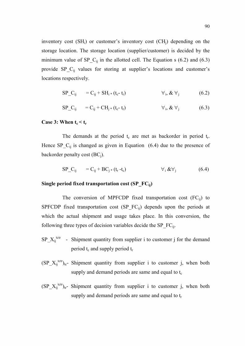
inventory cost (SHi) or customer�s inventory cost (CHj) depending on the
storage location. The storage location (supplier/customer) is decided by the
minimum value of SP_Cij in the allotted cell. The Equation s (6.2) and (6.3)
provide SP_Cij values for storing at supplier�s locations and customer�s
locations respectively.
SP_Cij = Cij + SHi * (tc- tr) �i, & �j (6.2)
SP_Cij = Cij + CHj * (tc- tr) �i, & �j (6.3)
Case 3: When tc < tr
The demands at the period tc are met as backorder in period tr.
Hence SP_Cij is changed as given in Equation (6.4) due to the presence of
backorder penalty cost (BCj).
SP_Cij = Cij + BCj * (tr -tc) �i &�j (6.4)
Single period fixed transportation cost (SP_FCij)
The conversion of MPFCDP fixed transportation cost (FCij) to
SPFCDP fixed transportation cost (SP_FCij) depends upon the periods at
which the actual shipment and usage takes place. In this conversion, the
following three types of decision variables decide the SP_FCij.
SP_Xijtctr
- Shipment quantity from supplier i to customer j for the demand
period tc and supply period tr
(SP_Xijtctr
)tc- Shipment quantity from supplier i to customer j, when both
supply and demand periods are same and equal to tc
(SP_Xijtctr
)tr- Shipment quantity from supplier i to customer j, when both
supply and demand periods are same and equal to tr
91
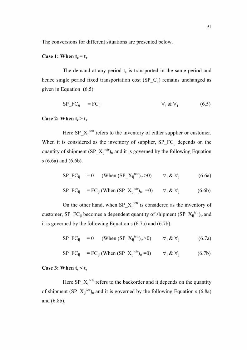
The conversions for different situations are presented below.
Case 1: When tc = tr
The demand at any period tc is transported in the same period and
hence single period fixed transportation cost (SP_Cij) remains unchanged as
given in Equation (6.5).
SP_FCij = FCij �i & �j (6.5)
Case 2: When tc > tr
Here SP_Xijtctr
refers to the inventory of either supplier or customer.
When it is considered as the inventory of supplier, SP_FCij depends on the
quantity of shipment (SP_Xijtctr
)tc and it is governed by the following Equation
s (6.6a) and (6.6b).
SP_FCij = 0 (When (SP_Xijtctr
)tc >0) �i & �j (6.6a)
SP_FCij = FCij (When (SP_Xijtctr
)tc =0) �i & �j (6.6b)
On the other hand, when SP_Xijtctr
is considered as the inventory of
customer, SP_FCij becomes a dependent quantity of shipment (SP_Xijtctr
)tr and
it is governed by the following Equation s (6.7a) and (6.7b).
SP_FCij = 0 (When (SP_Xijtctr
)tr >0) �i & �j (6.7a)
SP_FCij = FCij (When (SP_Xijtctr
)tr =0) �i & �j (6.7b)
Case 3: When tc < tr
Here SP_Xijtctr
refers to the backorder and it depends on the quantity
of shipment (SP_Xijtctr
)tr and it is governed by the following Equation s (6.8a)
and (6.8b).
92
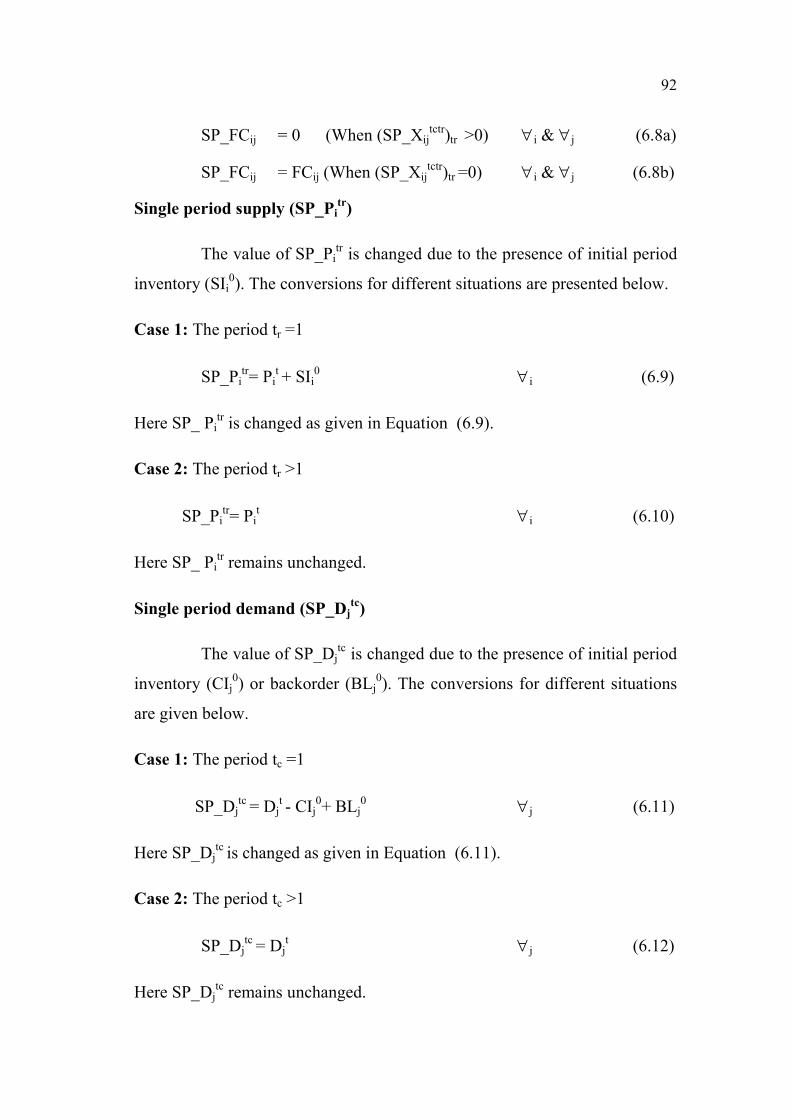
SP_FCij = 0 (When (SP_Xijtctr
)tr >0) �i & �j (6.8a)
SP_FCij = FCij (When (SP_Xijtctr
)tr =0) �i & �j (6.8b)
Single period supply (SP_Pitr
)
The value of SP_Pitr is changed due to the presence of initial period
inventory (SIi0). The conversions for different situations are presented below.
Case 1: The period tr =1
SP_Pitr= Pi
t + SIi
0 �i (6.9)
Here SP_ Pitr is changed as given in Equation (6.9).
Case 2: The period tr >1
SP_Pitr= Pi
t �i (6.10)
Here SP_ Pitr remains unchanged.
Single period demand (SP_Djtc
)
The value of SP_Djtc is changed due to the presence of initial period
inventory (CIj0) or backorder (BLj
0). The conversions for different situations
are given below.
Case 1: The period tc =1
SP_Djtc
= Djt - CIj
0+ BLj
0 �j (6.11)
Here SP_Djtc
is changed as given in Equation (6.11).
Case 2: The period tc >1
SP_Djtc
= Djt �j (6.12)
Here SP_Djtc remains unchanged.
93
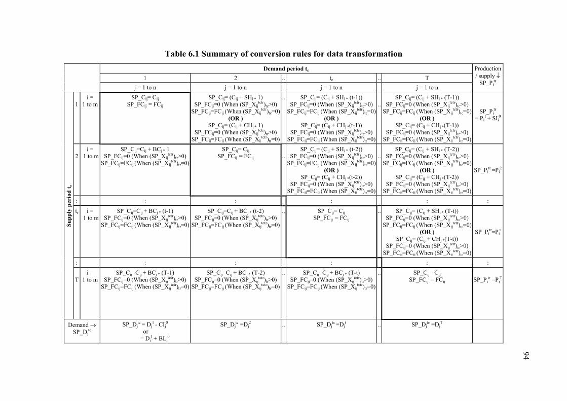
Table 6.1 presents the summary of the above rules of conversion in
the tabular form. The above modulations lend itself equivalent to the original
MPFCDP. However, as the demand of the customers is met either from the
inventories or as back orders, the fixed charge is not a constant. It depends on
the value of decision variables and it is either 0 or FCij depending upon the
period at which the actual shipment is made. This limits the usage of the
conventional FCTP solution procedures. However, the above conversion
provides a transformed data suitable for allocating the shipment quantities and
subsequently deriving a feasible MPFCDP distribution schedule in the SA
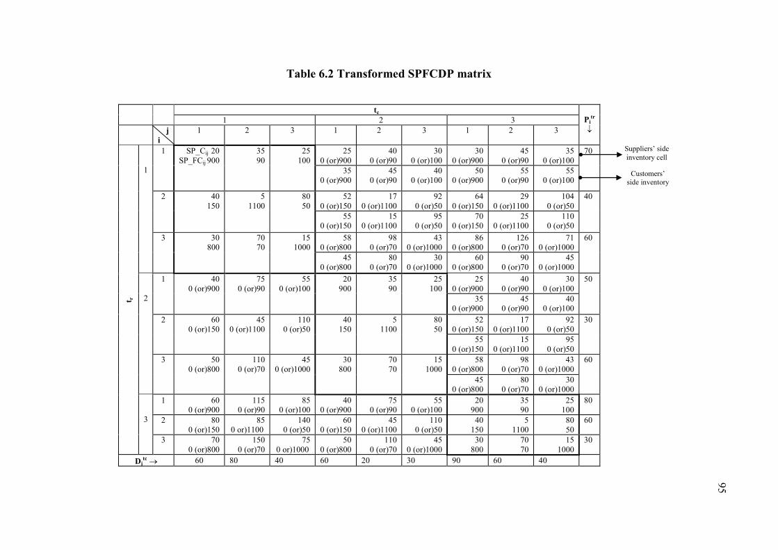
routine, which is delineated in the Stage II. Table 6.2 shows the SPFCDP data
matrix for the data of example problem given in chapter 4 (section 4.2).
94
94
Table 6.1 Summary of conversion rules for data transformation
Demand period tc Production
/ supply �
SP_Pitr
1 2 .. tc .. T
j = 1 to n j = 1 to n j = 1 to n j = 1 to n
Su
pp
ly p
erio
d t
r
1
i =
1 to m
SP_Cij= Cij
SP_FCij = FCij
SP_Cij= (Cij + SHi * 1)
SP_FCij=0 (When (SP_Xijtctr)tc>0)
SP_FCij=FCij (When (SP_Xijtctr)tc=0)
(OR )
SP_Cij= (Cij + CHj * 1)
SP_FCij=0 (When (SP_Xijtctr)tr>0)
SP_FCij=FCij (When (SP_Xijtctr)tr=0)
.. SP_Cij= (Cij + SHi * (t-1))
SP_FCij=0 (When (SP_Xijtctr)tc>0)
SP_FCij=FCij (When (SP_Xijtctr)tc=0)
(OR )
SP_Cij= (Cij + CHj *(t-1))
SP_FCij=0 (When (SP_Xijtctr)tr>0)
SP_FCij=FCij (When (SP_Xijtctr)tr=0)
..
SP_Cij= (Cij + SHi * (T-1))
SP_FCij=0 (When (SP_Xijtctr)tc>0)
SP_FCij=FCij (When (SP_Xijtctr)tc=0)
(OR )
SP_Cij= (Cij + CHj *(T-1))
SP_FCij=0 (When (SP_Xijtctr)tr>0)
SP_FCij=FCij (When (SP_Xijtctr)tr=0)
SP_Pitr
= Pi1 + SIi
0
2
i =
1 to m
SP_Cij=Cij + BCj * 1
SP_FCij=0 (When (SP_Xijtctr)tr>0)
SP_FCij=FCij (When (SP_Xijtctr)tr=0)
SP_Cij= Cij
SP_FCij = FCij ..
SP_Cij= (Cij + SHi * (t-2))
SP_FCij=0 (When (SP_Xijtctr)tc>0)
SP_FCij=FCij (When (SP_Xijtctr)tc=0)
(OR )
SP_Cij= (Cij + CHj *(t-2))
SP_FCij=0 (When (SP_Xijtctr)tr>0)
SP_FCij=FCij (When (SP_Xijtctr)tr=0)
..
SP_Cij= (Cij + SHi * (T-2))
SP_FCij=0 (When (SP_Xijtctr)tc>0)
SP_FCij=FCij (When (SP_Xijtctr)tc=0)
(OR )
SP_Cij= (Cij + CHj *(T-2))
SP_FCij=0 (When (SP_Xijtctr)tr>0)
SP_FCij=FCij (When (SP_Xijtctr)tr=0)
SP_Pitr =Pi
2
: : : : : :
tr i =
1 to m
SP_Cij=Cij + BCj * (t-1)
SP_FCij=0 (When (SP_Xijtctr)tr>0)
SP_FCij=FCij (When (SP_Xijtctr)tr=0)
SP_Cij=Cij + BCj * (t-2)
SP_FCij=0 (When (SP_Xijtctr)tr>0)
SP_FCij=FCij (When (SP_Xijtctr)tr=0)
.. SP_Cij= Cij
SP_FCij = FCij
.. SP_Cij= (Cij + SHi * (T-t))
SP_FCij=0 (When (SP_Xijtctr)tc>0)
SP_FCij=FCij (When (SP_Xijtctr)tc=0)
(OR )
SP_Cij= (Cij + CHj *(T-t))
SP_FCij=0 (When (SP_Xijtctr)tr>0)
SP_FCij=FCij (When (SP_Xijtctr)tr=0)
SP_Pitr=Pi
t
: : : : : :
T
i =
1 to m
SP_Cij=Cij + BCj * (T-1)
SP_FCij=0 (When (SP_Xijtctr)tr>0)
SP_FCij=FCij (When (SP_Xijtctr)tr=0)
SP_Cij=Cij + BCj * (T-2)
SP_FCij=0 (When (SP_Xijtctr)tr>0)
SP_FCij=FCij (When (SP_Xijtctr)tr=0)
.. SP_Cij=Cij + BCj * (T-t)
SP_FCij=0 (When (SP_Xijtctr)tr>0)
SP_FCij=FCij (When (SP_Xijtctr)tr=0)
.. SP_Cij= Cij
SP_FCij = FCij SP_Pitr =Pi
T
Demand �
SP_Djtc
SP_Djtc = Dj
1 - CIj0
or
= Dj1 + BLj
0
SP_Djtc =Dj
2 .. SP_Djtc =Dj
t .. SP_Djtc =Dj
T
95
95
Table 6.2 Transformed SPFCDP matrix
tc
Pitr
�
1 2 3
j
i
1 2 3 1 2 3 1 2 3 t r
1
1 SP_Cij 20
SP_FCij 900
35
90
25
100
25
0 (or)900
40
0 (or)90
30
0 (or)100
30
0 (or)900
45
0 (or)90
35
0 (or)100
70
35
0 (or)900
45
0 (or)90
40
0 (or)100
50
0 (or)900
55
0 (or)90
55
0 (or)100
2 40
150
5
1100
80
50
52
0 (or)150
17
0 (or)1100
92
0 (or)50
64
0 (or)150
29
0 (or)1100
104
0 (or)50
40
55
0 (or)150
15
0 (or)1100
95
0 (or)50
70
0 (or)150
25
0 (or)1100
110
0 (or)50
3 30
800
70
70
15
1000
58
0 (or)800
98
0 (or)70
43
0 (or)1000
86
0 (or)800
126
0 (or)70
71
0 (or)1000
60
45
0 (or)800
80
0 (or)70
30
0 (or)1000
60
0 (or)800
90
0 (or)70
45
0 (or)1000
2
1 40
0 (or)900
75
0 (or)90
55
0 (or)100
20
900
35
90
25
100
25
0 (or)900
40
0 (or)90
30
0 (or)100
50
35
0 (or)900
45
0 (or)90
40
0 (or)100
2 60
0 (or)150
45
0 (or)1100
110
0 (or)50
40
150
5
1100
80
50
52
0 (or)150
17
0 (or)1100
92
0 (or)50
30
55
0 (or)150
15
0 (or)1100
95
0 (or)50
3 50
0 (or)800
110
0 (or)70
45
0 (or)1000
30
800
70
70
15
1000
58
0 (or)800
98
0 (or)70
43
0 (or)1000
60
45
0 (or)800
80
0 (or)70
30
0 (or)1000
3
1 60
0 (or)900
115
0 (or)90
85
0 (or)100
40
0 (or)900
75
0 (or)90
55
0 (or)100
20
900
35
90
25
100
80
2 80
0 (or)150
85
0 or)1100
140
0 (or)50
60
0 (or)150
45
0 (or)1100
110
0 (or)50
40
150
5
1100
80
50
60
3 70
0 (or)800
150
0 (or)70
75
0 or)1000
50
0 (or)800
110
0 (or)70
45
0 (or)1000
30
800
70
70
15
1000
30
Djtc � 60 80 40 60 20 30 90 60 40
Suppliers� side
inventory cell
Customers�
side inventory
cell
96
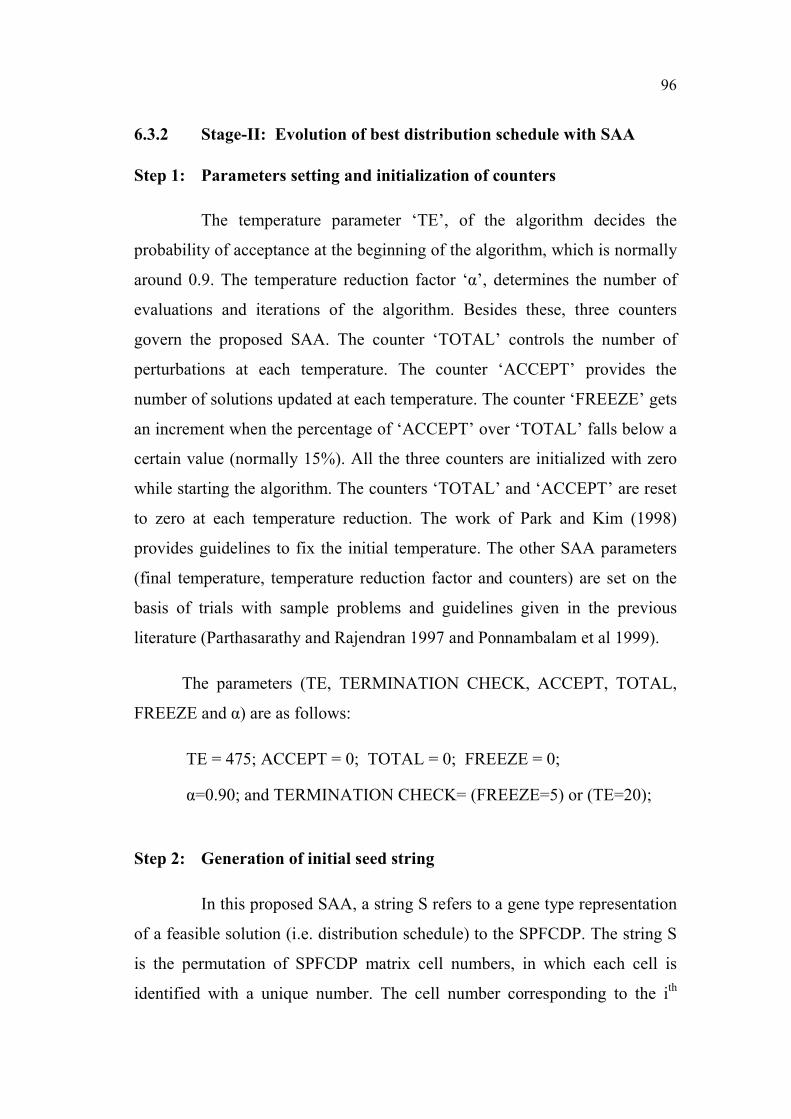
6.3.2 Stage-II: Evolution of best distribution schedule with SAA
Step 1: Parameters setting and initialization of counters
The temperature parameter �TE�, of the algorithm decides the
probability of acceptance at the beginning of the algorithm, which is normally
around 0.9. The temperature reduction factor ���, determines the number of
evaluations and iterations of the algorithm. Besides these, three counters
govern the proposed SAA. The counter �TOTAL� controls the number of
perturbations at each temperature. The counter �ACCEPT� provides the
number of solutions updated at each temperature. The counter �FREEZE� gets
an increment when the percentage of �ACCEPT� over �TOTAL� falls below a
certain value (normally 15%). All the three counters are initialized with zero
while starting the algorithm. The counters �TOTAL� and �ACCEPT� are reset
to zero at each temperature reduction. The work of Park and Kim (1998)
provides guidelines to fix the initial temperature. The other SAA parameters
(final temperature, temperature reduction factor and counters) are set on the
basis of trials with sample problems and guidelines given in the previous
literature (Parthasarathy and Rajendran 1997 and Ponnambalam et al 1999).
The parameters (TE, TERMINATION CHECK, ACCEPT, TOTAL,
FREEZE and �) are as follows:
TE = 475; ACCEPT = 0; TOTAL = 0; FREEZE = 0;
�=0.90; and TERMINATION CHECK= (FREEZE=5) or (TE=20);
Step 2: Generation of initial seed string
In this proposed SAA, a string S refers to a gene type representation
of a feasible solution (i.e. distribution schedule) to the SPFCDP. The string S
is the permutation of SPFCDP matrix cell numbers, in which each cell is
identified with a unique number. The cell number corresponding to the ith

97
supplier of supply period tr and the jth
customer of demand period tc is fixed by
using the Equation (6.13) given below.
Cell number ={(tr -1) * m * n* T} + {(i-1) * (n*T)} + {(tc -1) * n} + j (6.13)
The total number of cells in the SPFCDP, which is also equal to the
length of the string S, thus becomes (m*T)*(n*T). Table 6.3 illustrates the
SPFCDP matrix cell numbers for the illustration problem given in Tables
4.1a, 4.1b and 4.1c. When the supply and demand are in same period (i.e. tc =
tr), then they form T diagonal sub matrices of size m*n (shown as rectangles
with dark borders in Table 6.3). The number of cells in the diagonal matrix
thus becomes equal to (m*n*T). Any value in the cell below the diagonal
matrix indicates the unfilled demand (backorder) of customer j in the period
tc, which is met by the supplier i during the next period tc+1. On the other
hand, any value in the cell above the diagonal matrix indicates the excess
supply (inventory) of supplier i in the period tr, which is either kept at the
location of the supplier i itself or delivered to customer j and stored at the
customer�s location.
Table 6.3 SPFCDP cell numbers matrix
tc
1 2 3
j
i
1 2 3 1 2 3 1 2 3
t r
1
1 1 2 3 4 5 6 7 8 9
2 10 11 12 13 14 15 16 17 18
3 19 20 21 22 23 24 25 26 27
2
1 28 29 30 31 32 33 34 35 36
2 37 38 39 40 41 42 43 44 45
3 46 47 48 49 50 51 52 53 54
3
1 55 56 57 58 59 60 61 62 63
2 64 65 66 67 68 69 70 71 72
3 73 74 75 76 77 78 79 80 81
98
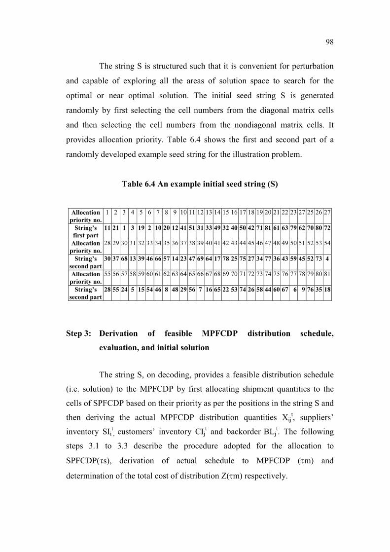
The string S is structured such that it is convenient for perturbation
and capable of exploring all the areas of solution space to search for the
optimal or near optimal solution. The initial seed string S is generated
randomly by first selecting the cell numbers from the diagonal matrix cells
and then selecting the cell numbers from the nondiagonal matrix cells. It
provides allocation priority. Table 6.4 shows the first and second part of a
randomly developed example seed string for the illustration problem.
Table 6.4 An example initial seed string (S)
Allocation
priority no.
1 2 3 4 5 6 7 8 9 10 11 12 13 14 15 16 17 18 19 20 21 22 23 27 25 26 27
String�s
first part
11 21 1 3 19 2 10 20 12 41 51 31 33 49 32 40 50 42 71 81 61 63 79 62 70 80 72
Allocation
priority no.
28 29 30 31 32 33 34 35 36 37 38 39 40 41 42 43 44 45 46 47 48 49 50 51 52 53 54
String�s
second part
30 37 68 13 39 46 66 57 14 23 47 69 64 17 78 25 75 27 34 77 36 43 59 45 52 73 4
Allocation
priority no.
55 56 57 58 59 60 61 62 63 64 65 66 67 68 69 70 71 72 73 74 75 76 77 78 79 80 81
String�s
second part
28 55 24 5 15 54 46 8 48 29 56 7 16 65 22 53 74 26 58 44 60 67 6 9 76 35 18
Step 3: Derivation of feasible MPFCDP distribution schedule,
evaluation, and initial solution
The string S, on decoding, provides a feasible distribution schedule
(i.e. solution) to the MPFCDP by first allocating shipment quantities to the
cells of SPFCDP based on their priority as per the positions in the string S and
then deriving the actual MPFCDP distribution quantities Xijt, suppliers�
inventory SIit, customers� inventory CIj
t and backorder BLj
t. The following
steps 3.1 to 3.3 describe the procedure adopted for the allocation to
SPFCDP(�s), derivation of actual schedule to MPFCDP (�m) and
determination of the total cost of distribution Z(�m) respectively.
99
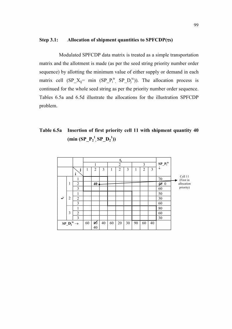
Step 3.1: Allocation of shipment quantities to SPFCDP(����s)
Modulated SPFCDP data matrix is treated as a simple transportation
matrix and the allotment is made (as per the seed string priority number order
sequence) by allotting the minimum value of either supply or demand in each
matrix cell (SP_Xij= min (SP_Pitr
, SP_Djtc)). The allocation process is
continued for the whole seed string as per the priority number order sequence.
Tables 6.5a and 6.5d illustrate the allocations for the illustration SPFCDP
problem.
Table 6.5a Insertion of first priority cell 11 with shipment quantity 40
(min (SP_P21
, SP_D21))
tc
SP_Pitr
�1 2 3
j
i
1 2 3 1 2 3 1 2 3
tr
1
1 70
2 40 40 0
3 60
2
1 50
2 30
3 60
3
1 80
2 60
3 30
SP_Djtc� 60 80
40
40 60 20 30 90 60 40
Cell 11
(First in
allocation
priority)
100
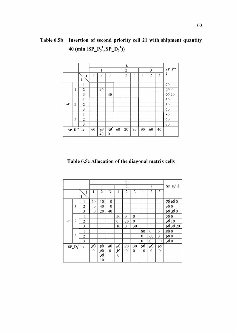
Table 6.5b Insertion of second priority cell 21 with shipment quantity
40 (min (SP_P31, SP_D3
1))
Table 6.5c Allocation of the diagonal matrix cells
tc
SP_Pitr �1 2 3
j
i
1 2 3 1 2 3 1 2 3
t r
1
1 60 10 0 70 60 0
2 0 40 0 40 0
3 0 20 40 60 20 0
2
1 50 0 0 50 0
2 0 20 0 30 10
3 10 0 30 60 30 20
3
1 80 0 0 80 0
2 0 60 0 60 0
3 0 0 30 30 0
SP_Djtc� 60
0
80
40
30
10
40
0
60
50
0
20
0
30
0
90
10
60
0
40
0
tc
SP_Pitr
�1 2 3
j
i
1 2 3 1 2 3 1 2 3
tr
1
1 70
2 40 40 0
3 40 60 20
2
1 50
2 30
3 60
3
1 80
2 60
3 30
SP_Djtc� 60 80
40
40
0
60 20 30 90 60 40
101
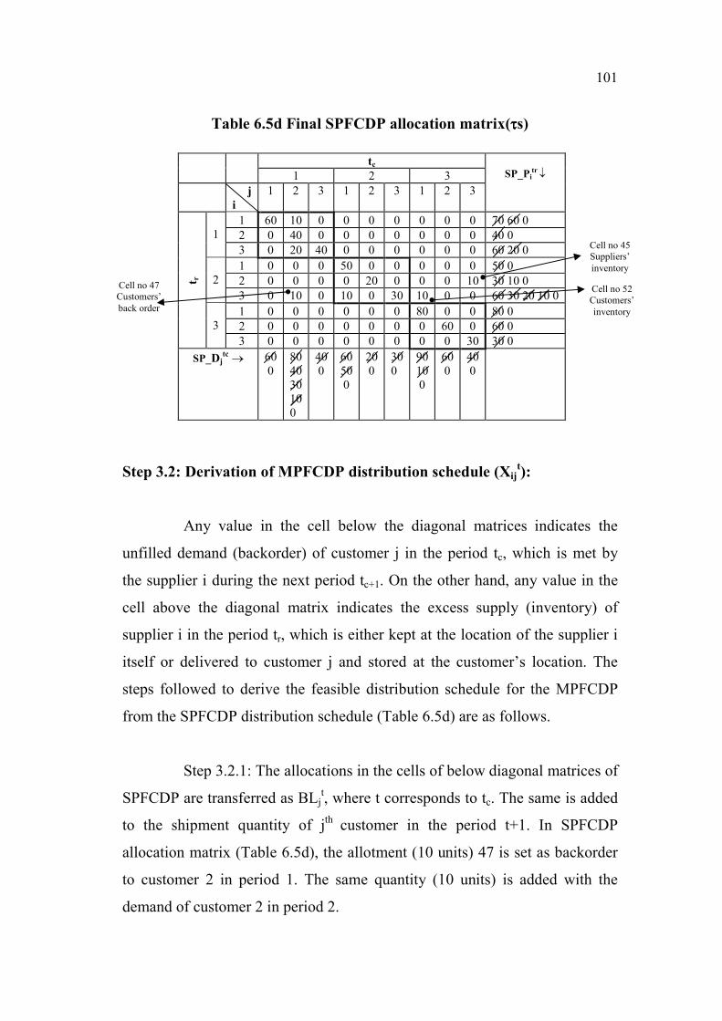
Table 6.5d Final SPFCDP allocation matrix(����s)
Step 3.2: Derivation of MPFCDP distribution schedule (Xijt):
Any value in the cell below the diagonal matrices indicates the
unfilled demand (backorder) of customer j in the period tc, which is met by
the supplier i during the next period tc+1. On the other hand, any value in the
cell above the diagonal matrix indicates the excess supply (inventory) of
supplier i in the period tr, which is either kept at the location of the supplier i
itself or delivered to customer j and stored at the customer�s location. The
steps followed to derive the feasible distribution schedule for the MPFCDP
from the SPFCDP distribution schedule (Table 6.5d) are as follows.
Step 3.2.1: The allocations in the cells of below diagonal matrices of
SPFCDP are transferred as BLjt, where t corresponds to tc. The same is added
to the shipment quantity of jth
customer in the period t+1. In SPFCDP
allocation matrix (Table 6.5d), the allotment (10 units) 47 is set as backorder
to customer 2 in period 1. The same quantity (10 units) is added with the
demand of customer 2 in period 2.
tc
SP_Pitr �1 2 3
j
i
1 2 3 1 2 3 1 2 3 t r
1
1 60 10 0 0 0 0 0 0 0 70 60 0
2 0 40 0 0 0 0 0 0 0 40 0
3 0 20 40 0 0 0 0 0 0 60 20 0
2
1 0 0 0 50 0 0 0 0 0 50 0
2 0 0 0 0 20 0 0 0 10 30 10 0
3 0 10 0 10 0 30 10 0 0 60 30 20 10 0
3
1 0 0 0 0 0 0 80 0 0 80 0
2 0 0 0 0 0 0 0 60 0 60 0
3 0 0 0 0 0 0 0 0 30 30 0
SP_Djtc� 60
0
80
40
30
10
0
40
0
60
50
0
20
0
30
0
90
10
0
60
0
40
0
Cell no 45
Suppliers�
inventory
Cell no 52
Customers�
inventory
Cell no 47
Customers�
back order

102
Step 3.2.3: The allocations in the cells of above diagonal matrices of
SPFCDP are transferred as supplier�s inventory or customer�s inventory. It is
decided by the minimum SP_Cij value (minimum value of SP_Cij in the
supplier�s side and customer�s side inventory cell) and not by SP_FCij value.
It is because, SP_FCij value is either 0 or FCij depending upon the period at
which the actual shipment is made.
Case 1: Storage at the suppliers� side itself
The allocations in the cells of above diagonal matrices of SPFCDP
are transferred as supplier�s inventory SIit, where t corresponds to tc. The
same is added to the shipment quantity of ith
supplier in the period t+1. In
Table 6.5d, the allotment (10 units) in cell number 45 is set as supplier�s
inventory. Because the SP_Cij minimum is 92 (supplier�s side SP_Cij =92 and
customer�s side SP_Cij =95). This supplier�s inventory belongs to supplier 2
in period 2. The same quantity (10 units) is added with the supply of supplier
2 in period 3.
Case 2: Storage at the customers� side
The allocations in the cells of above diagonal matrices of SPFCDP
are transferred as CIjt in the period t itself, where t corresponds to tr. The same
is subtracted from the demand quantity of jth
customer in the period t+1. In
Table 6.5d, the allotment (10 units) in cell number 52 is set as customer�s
inventory. Because the SP_Cij minimum is 45 (supplier�s side SP_Cij =58 and
customer�s side SP_Cij =45). This customer�s inventory belongs to customer 1
in period 2. The same quantity (10 units) is subtracted from the demand of
customer 1 in period 3.
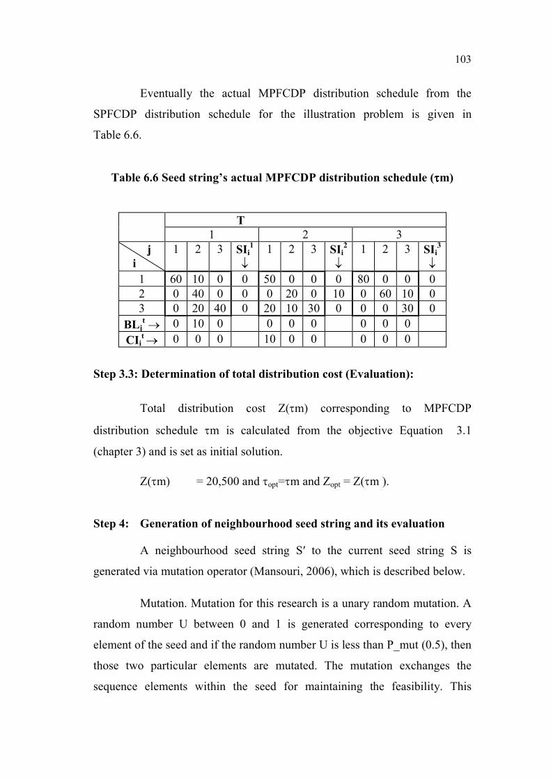
103
Eventually the actual MPFCDP distribution schedule from the
SPFCDP distribution schedule for the illustration problem is given in
Table 6.6.
Table 6.6 Seed string�s actual MPFCDP distribution schedule (����m)
T
1 2 3
j
i
1 2 3 SIi1
�
1 2 3 SIi2
�
1 2 3 SIi3
�
1 60 10 0 0 50 0 0 0 80 0 0 0
2 0 40 0 0 0 20 0 10 0 60 10 0
3 0 20 40 0 20 10 30 0 0 0 30 0
BLjt� 0 10 0 0 0 0 0 0 0
CIit � 0 0 0 10 0 0 0 0 0
Step 3.3: Determination of total distribution cost (Evaluation):
Total distribution cost Z(�m) corresponding to MPFCDP
distribution schedule �m is calculated from the objective Equation 3.1
(chapter 3) and is set as initial solution.
Z(�m) = 20,500 and �opt=�m and Zopt = Z(�m ).
Step 4: Generation of neighbourhood seed string and its evaluation
A neighbourhood seed string S� to the current seed string S is
generated via mutation operator (Mansouri, 2006), which is described below.
Mutation. Mutation for this research is a unary random mutation. A
random number U between 0 and 1 is generated corresponding to every
element of the seed and if the random number U is less than P_mut (0.5), then
those two particular elements are mutated. The mutation exchanges the
sequence elements within the seed for maintaining the feasibility. This
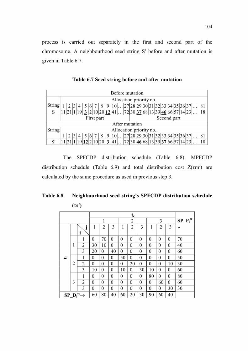
104
process is carried out separately in the first and second part of the
chromosome. A neighbourhood seed string S� before and after mutation is
given in Table 6.7.
Table 6.7 Seed string before and after mutation
Before mutation
StringAllocation priority no.
1 2 3 4 5 6 7 8 9 10 � 27 28 29 30 31 32 33 34 35 36 37 � 81
S 11 21 1 19 3 2 10 20 12 41 � 72 30 37 68 13 39 46 66 57 14 23 ... 18
First part Second part
After mutation
String Allocation priority no.
1 2 3 4 5 6 7 8 9 10 � 27 28 29 30 31 32 33 34 35 36 37 � 81
S� 11 21 1 19 12 2 10 20 3 41 � 72 30 46 68 13 39 37 66 57 14 23 ... 18
The SPFCDP distribution schedule (Table 6.8), MPFCDP
distribution schedule (Table 6.9) and total distribution cost Z(�m�) are
calculated by the same procedure as used in previous step 3.
Table 6.8 Neighbourhood seed string�s SPFCDP distribution schedule
(����s�)
tc
SP_Pitr
�
1 2 3
t r
j
i
1 2 3 1 2 3 1 2 3
1
1 0 70 0 0 0 0 0 0 0 70
2 30 10 0 0 0 0 0 0 0 40
3 20 0 40 0 0 0 0 0 0 60
2
1 0 0 0 50 0 0 0 0 0 50
2 0 0 0 0 20 0 0 0 10 30
3 10 0 0 10 0 30 10 0 0 60
3
1 0 0 0 0 0 0 80 0 0 80
2 0 0 0 0 0 0 0 60 0 60
3 0 0 0 0 0 0 0 0 30 30
SP_Djtc� 60 80 40 60 20 30 90 60 40
105
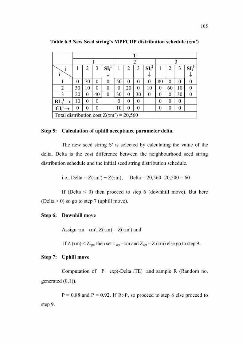
Table 6.9 New Seed string�s MPFCDP distribution schedule (����m�)
T
1 2 3
j
i
1 2 3 SIi1
�
1 2 3 SIi2
�
1 2 3 SIi3
�
1 0 70 0 0 50 0 0 0 80 0 0 0
2 30 10 0 0 0 20 0 10 0 60 10 0
3 20 0 40 0 30 0 30 0 0 0 30 0
BLjt� 10 0 0 0 0 0 0 0 0
CIit � 0 0 0 10 0 0 0 0 0
Total distribution cost Z(�m�) = 20,560
Step 5: Calculation of uphill acceptance parameter delta.
The new seed string S� is selected by calculating the value of the
delta. Delta is the cost difference between the neighbourhood seed string
distribution schedule and the initial seed string distribution schedule.
i.e., Delta = Z(�m�) − Z(�m); Delta = 20,560- 20,500 = 60
If (Delta � 0) then proceed to step 6 (downhill move). But here
(Delta > 0) so go to step 7 (uphill move).
Step 6: Downhill move
Assign �m =�m�, Z(�m) = Z(�m�) and
If Z (�m) < Zopt, then set � opt =�m and Zopt = Z (�m) else go to step 9.
Step 7: Uphill move
Computation of /TE)exp(-Delta P � and sample R (Random no.
generated (0,1)).
P = 0.88 and P = 0.92. If PR� , so proceed to step 8 else proceed to
step 9.
106
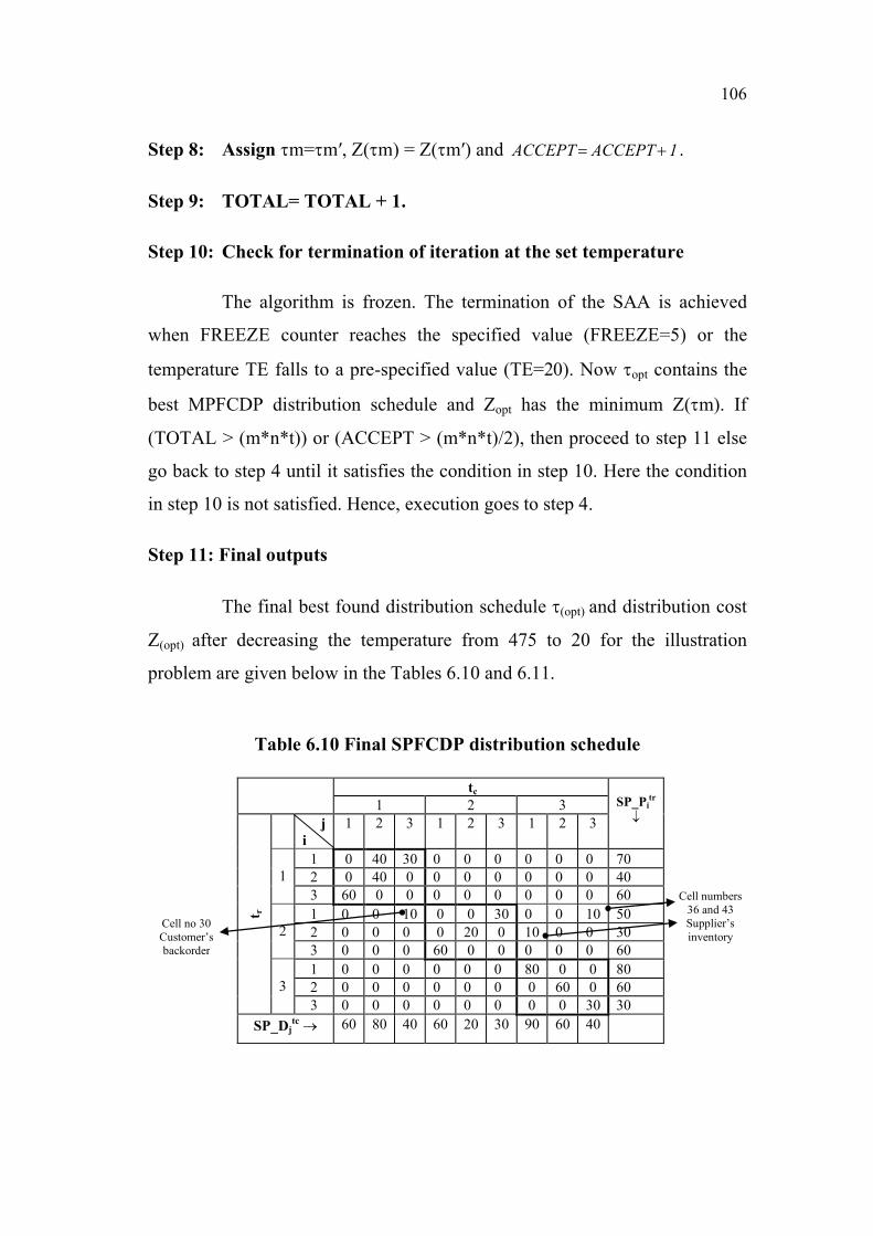
Step 8: Assign �m=�m�, Z(�m) = Z(�m�) and 1 ACCEPT ACCEPT � .
Step 9: TOTAL= TOTAL + 1.
Step 10: Check for termination of iteration at the set temperature
The algorithm is frozen. The termination of the SAA is achieved
when FREEZE counter reaches the specified value (FREEZE=5) or the
temperature TE falls to a pre-specified value (TE=20). Now �opt contains the
best MPFCDP distribution schedule and Zopt has the minimum Z(�m). If
(TOTAL > (m*n*t)) or (ACCEPT > (m*n*t)/2), then proceed to step 11 else
go back to step 4 until it satisfies the condition in step 10. Here the condition
in step 10 is not satisfied. Hence, execution goes to step 4.
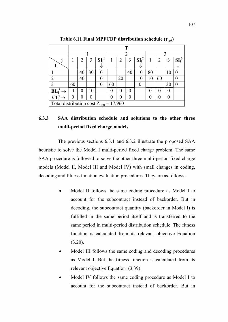
Step 11: Final outputs
The final best found distribution schedule �(opt) and distribution cost
Z(opt) after decreasing the temperature from 475 to 20 for the illustration
problem are given below in the Tables 6.10 and 6.11.
Table 6.10 Final SPFCDP distribution schedule
tc
SP_Pitr
�1 2 3
t r
j
i
1 2 3 1 2 3 1 2 3
1
1 0 40 30 0 0 0 0 0 0 70
2 0 40 0 0 0 0 0 0 0 40
3 60 0 0 0 0 0 0 0 0 60
2
1 0 0 10 0 0 30 0 0 10 50
2 0 0 0 0 20 0 10 0 0 30
3 0 0 0 60 0 0 0 0 0 60
3
1 0 0 0 0 0 0 80 0 0 80
2 0 0 0 0 0 0 0 60 0 60
3 0 0 0 0 0 0 0 0 30 30
SP_Djtc� 60 80 40 60 20 30 90 60 40
Cell numbers
36 and 43
Supplier’s
inventory
Cell no 30
Customer’s
backorder
107
Table 6.11 Final MPFCDP distribution schedule (����opt)
T
1 2 3
j
i
1 2 3 SIi1
�
1 2 3 SIi2
�
1 2 3 SIi3
�
1 40 30 0 40 10 80 10 0
2 40 0 20 10 10 60 0
3 60 0 60 0 30 0
BLjt� 0 0 10 0 0 0 0 0 0
CIit � 0 0 0 0 0 0 0 0 0
Total distribution cost Z opt = 17,960
6.3.3 SAA distribution schedule and solutions to the other three
multi-period fixed charge models
The previous sections 6.3.1 and 6.3.2 illustrate the proposed SAA
heuristic to solve the Model I multi-period fixed charge problem. The same
SAA procedure is followed to solve the other three multi-period fixed charge
models (Model II, Model III and Model IV) with small changes in coding,
decoding and fitness function evaluation procedures. They are as follows:
� Model II follows the same coding procedure as Model I to
account for the subcontract instead of backorder. But in
decoding, the subcontract quantity (backorder in Model I) is
fulfilled in the same period itself and is transferred to the
same period in multi-period distribution schedule. The fitness
function is calculated from its relevant objective Equation
(3.20).
� Model III follows the same coding and decoding procedures
as Model I. But the fitness function is calculated from its
relevant objective Equation (3.39).
� Model IV follows the same coding procedure as Model I to
account for the subcontract instead of backorder. But in
108
decoding, the subcontract quantity (backorder in Model I) is
fulfilled in the same period itself and is transferred to the
same period in multi-period distribution schedule. The fitness
function is calculated from its relevant objective
Equation (3.58).
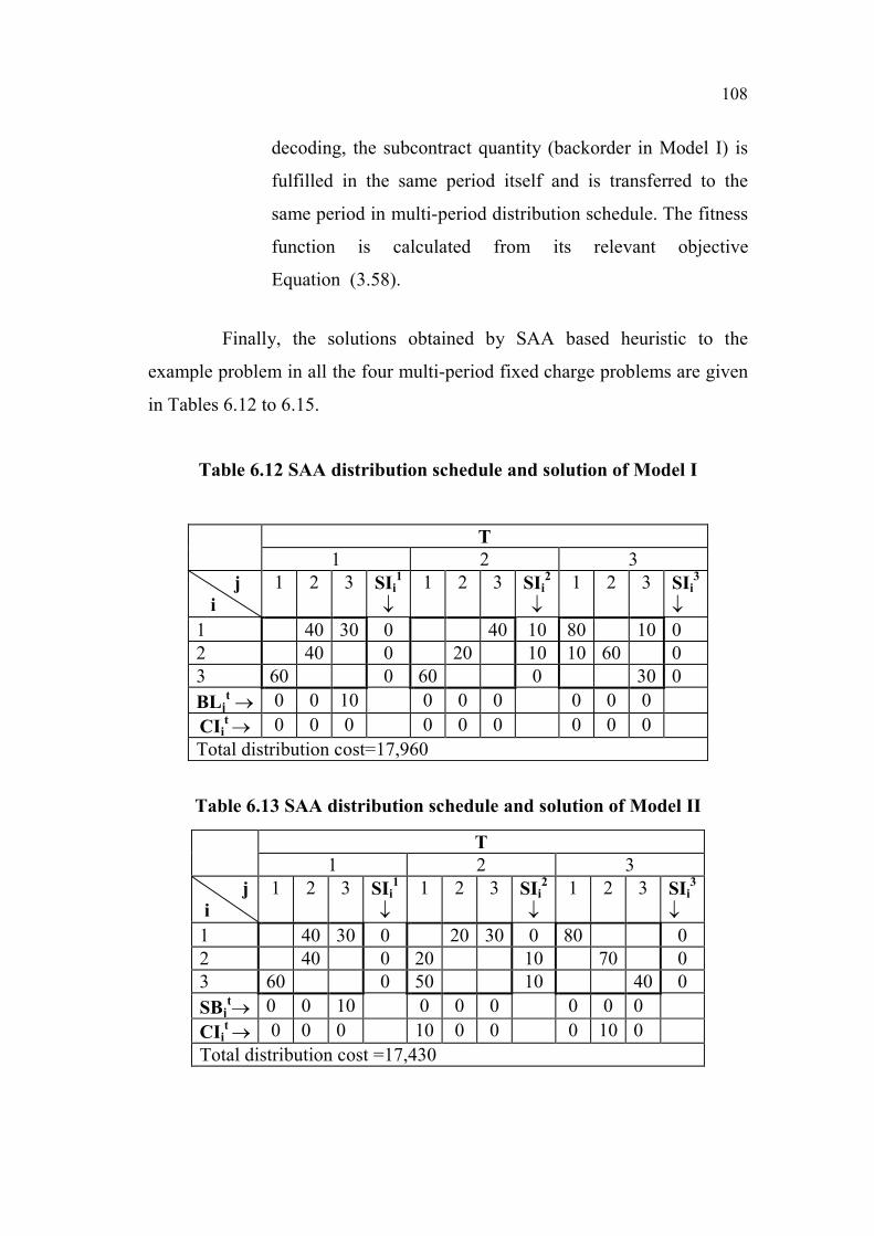
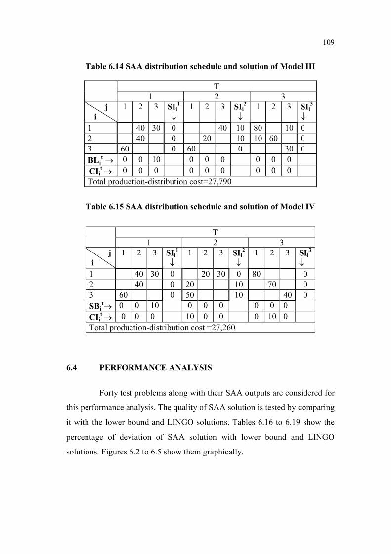
Finally, the solutions obtained by SAA based heuristic to the
example problem in all the four multi-period fixed charge problems are given
in Tables 6.12 to 6.15.
Table 6.12 SAA distribution schedule and solution of Model I
T
1 2 3
j
i
1 2 3 SIi1
�
1 2 3 SIi2
�
1 2 3 SIi3
�
1 40 30 0 40 10 80 10 0
2 40 0 20 10 10 60 0
3 60 0 60 0 30 0
BLjt� 0 0 10 0 0 0 0 0 0
CIit � 0 0 0 0 0 0 0 0 0
Total distribution cost=17,960
Table 6.13 SAA distribution schedule and solution of Model II
T
1 2 3
j
i
1 2 3 SIi1
�
1 2 3 SIi2
�
1 2 3 SIi3
�
1 40 30 0 20 30 0 80 0
2 40 0 20 10 70 0
3 60 0 50 10 40 0
SBjt� 0 0 10 0 0 0 0 0 0
CIit � 0 0 0 10 0 0 0 10 0
Total distribution cost =17,430
109
Table 6.14 SAA distribution schedule and solution of Model III
T
1 2 3
j
i
1 2 3 SIi1
�
1 2 3 SIi2
�
1 2 3 SIi3
�
1 40 30 0 40 10 80 10 0
2 40 0 20 10 10 60 0
3 60 0 60 0 30 0
BLjt� 0 0 10 0 0 0 0 0 0
CIit � 0 0 0 0 0 0 0 0 0
Total production-distribution cost=27,790
Table 6.15 SAA distribution schedule and solution of Model IV
T
1 2 3
j
i
1 2 3 SIi1
�
1 2 3 SIi2
�
1 2 3 SIi3
�
1 40 30 0 20 30 0 80 0
2 40 0 20 10 70 0
3 60 0 50 10 40 0
SBjt� 0 0 10 0 0 0 0 0 0
CIit � 0 0 0 10 0 0 0 10 0
Total production-distribution cost =27,260
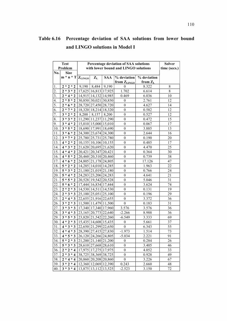
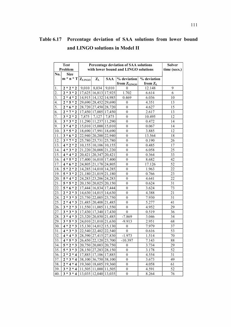
6.4 PERFORMANCE ANALYSIS
Forty test problems along with their SAA outputs are considered for
this performance analysis. The quality of SAA solution is tested by comparing
it with the lower bound and LINGO solutions. Tables 6.16 to 6.19 show the
percentage of deviation of SAA solution with lower bound and LINGO
solutions. Figures 6.2 to 6.5 show them graphically.
110
Table 6.16 Percentage deviation of SAA solutions from lower bound
and LINGO solutions in Model I
Test
Problem
Percentage deviation of SAA solutions
with lower bound and LINGO solutions
Solver
time (secs.)
No. Size
m * n * T ZLINGO ZL SAA % deviation
from ZLINGO
% deviation
from ZL
1. 2 * 2 * 2 9,190 8,484 9,190 0 8.322 8
2. 2 * 3 * 2 17,625 16,813 17,925 1.702 6.614 8
3. 2 * 4 * 2 14,915 14,132 14,985 0.469 6.036 10
4. 2 * 5 * 2 30,850 30,021 30,850 0 2.761 12
5. 2 * 6 * 2 28,720 27,450 28,720 0 4.627 14
6. 2 * 7 * 2 18,320 18,214 18,320 0 0.582 12
7. 3 * 2 * 2 8,200 8,157 8,200 0 0.527 12
8. 3 * 3 * 2 11,290 11,237 11,290 0 0.472 15
9. 3 * 4 * 2 15,010 15,000 15,010 0 0.067 17
10. 3 * 5 * 2 18,690 17,991 18,690 0 3.885 13
11. 3 * 6 * 2 24,300 23,674 24,300 0 2.644 16
12. 3 * 7 * 2 25,780 25,731 25,780 0 0.190 20
13. 4 * 2 * 2 10,155 10,106 10,155 0 0.485 17
14. 4 * 3 * 2 21,620 20,695 21,620 0 4.470 25
15. 4 * 4 * 2 20,421 20,347 20,421 0 0.364 30
16. 4 * 5 * 2 20,460 20,310 20,460 0 0.739 38
17. 4 * 6 * 2 24,805 21,178 24,805 0 17.126 47
18. 5 * 2 * 2 14,285 14,010 14,285 0 1.963 22
19. 5 * 3 * 2 21,180 21,019 21,180 0 0.766 24
20. 5 * 4 * 2 24,283 23,206 24,283 0 4.641 21
21. 5 * 5 * 2 20,528 19,542 20,528 0 5.046 31
22. 5 * 6 * 2 17,444 16,834 17,444 0 3.624 74
23. 2 * 2 * 3 14,530 14,511 14,530 0 0.131 19
24. 2 * 3 * 3 25,100 25,051 25,100 0 0.196 29
25. 2 * 4 * 3 22,655 21,916 22,655 0 3.372 36
26. 3 * 2 * 3 11,500 11,479 11,500 0 0.183 31
27. 3 * 3 * 3 17,340 17,340 17,960 3.576 3.576 36
28. 3 * 4 * 3 23,165 20,773 22,640 -2.266 8.988 36
29. 3 * 5 * 3 23,820 21,542 22,260 -6.549 3.333 69
30. 4 * 2 * 3 15,435 14,608 15,435 0 5.661 37
31. 4 * 3 * 3 22,650 21,299 22,650 0 6.343 55
32. 4 * 4 * 3 28,390 27,415 27,830 -1.973 1.514 73
33. 4 * 5 * 3 26,120 24,266 24,805 -5.034 2.221 91
34. 5 * 2 * 3 21,200 21,140 21,200 0 0.284 26
35. 5 * 3 * 3 28,610 27,668 28,610 0 3.405 46
36. 2 * 2 * 4 17,975 17,275 17,975 0 4.052 33
37. 2 * 3 * 4 38,725 38,369 38,725 0 0.928 49
38. 2 * 4 * 4 20,860 20,208 20,860 0 3.226 67
39. 3 * 2 * 4 12,360 12,069 12,390 0.243 2.660 48
40. 3 * 3 * 4 13,875 13,112 13,525 -2.523 3.150 72
111
Table 6.17 Percentage deviation of SAA solutions from lower bound
and LINGO solutions in Model II
Test
Problem
Percentage deviation of SAA solutions
with lower bound and LINGO solutions
Solver
time (secs.)
No. Size
m * n * T ZLINGO ZL SAA % deviation
from ZLINGO
% deviation
from ZL
1. 2 * 2 * 2 9,010 8,034 9,010 0 12.148 9
2. 2 * 3 * 2 17,625 16,813 17,925 1.702 6.614 6
3. 2 * 4 * 2 14,915 14,132 14,985 0.469 6.036 10
4. 2 * 5 * 2 29,690 28,452 29,690 0 4.351 13
5. 2 * 6 * 2 28,720 27,450 28,720 0 4.627 15
6. 2 * 7 * 2 17,450 17,005 17,450 0 2.617 13
7. 3 * 2 * 2 7,875 7,127 7,875 0 10.495 12
8. 3 * 3 * 2 11,290 11,237 11,290 0 0.472 14
9. 3 * 4 * 2 15,010 15,000 15,010 0 0.067 14
10. 3 * 5 * 2 18,690 17,991 18,690 0 3.885 12
11. 3 * 6 * 2 22,940 20,200 22,940 0 13.564 18
12. 3 * 7 * 2 25,780 25,731 25,780 0 0.190 26
13. 4 * 2 * 2 10,155 10,106 10,155 0 0.485 17
14. 4 * 3 * 2 21,220 20,008 21,220 0 6.058 25
15. 4 * 4 * 2 20,421 20,347 20,421 0 0.364 33
16. 4 * 5 * 2 17,400 16,010 17,400 0 8.682 42
17. 4 * 6 * 2 24,805 21,178 24,805 0 17.126 52
18. 5 * 2 * 2 14,285 14,010 14,285 0 1.963 22
19. 5 * 3 * 2 21,180 21,019 21,180 0 0.766 23
20. 5 * 4 * 2 24,283 23,206 24,283 0 4.641 22
21. 5 * 5 * 2 20,150 20,025 20,150 0 0.624 31
22. 5 * 6 * 2 17,444 16,834 17,444 0 3.624 73
23. 2 * 2 * 3 14,630 14,015 14,630 0 4.388 21
24. 2 * 3 * 3 23,750 22,005 23,750 0 7.930 31
25. 2 * 4 * 3 21,485 20,408 21,485 0 5.277 41
26. 3 * 2 * 3 11,550 11,005 11,550 0 4.952 29
27. 3 * 3 * 3 17,430 17,340 17,430 0 0.519 36
28. 3 * 4 * 3 23,320 20,850 21,485 -7.869 3.046 34
29. 3 * 5 * 3 24,010 21,010 21,630 -9.913 2.951 68
30. 4 * 2 * 3 15,130 14,012 15,130 0 7.979 37
31. 4 * 3 * 3 22,540 22,402 22,540 0 0.616 53
32. 4 * 4 * 3 28,390 27,415 27,830 -1.973 1.514 70
33. 4 * 5 * 3 26,450 22,120 23,700 -10.397 7.143 88
34. 5 * 2 * 3 20,750 20,003 20,750 0 3.734 29
35. 5 * 3 * 3 28,150 27,283 28,150 0 3.178 52
36. 2 * 2 * 4 17,885 17,106 17,885 0 4.554 31
37. 2 * 3 * 4 38,100 36,750 38,100 0 3.673 49
38. 2 * 4 * 4 19,360 18,605 19,360 0 4.058 61
39. 3 * 2 * 4 11,505 11,000 11,505 0 4.591 52
40. 3 * 3 * 4 13,035 12,040 13,035 0 8.264 76
112
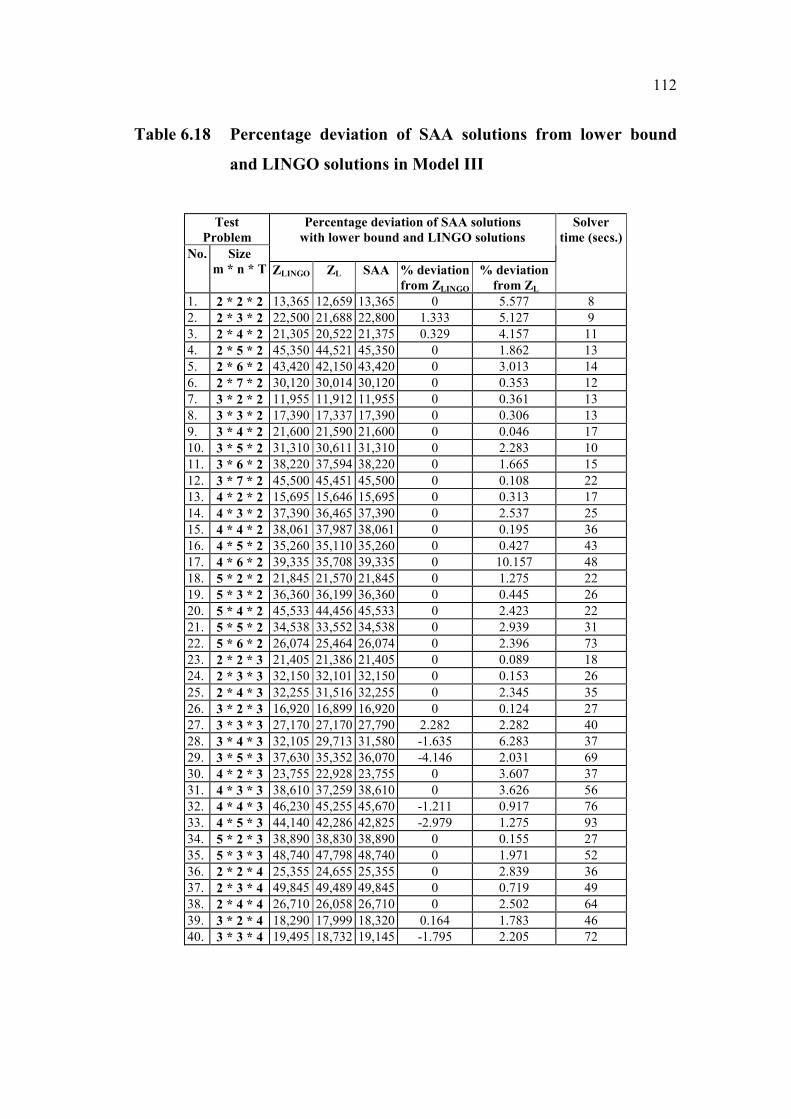
Table 6.18 Percentage deviation of SAA solutions from lower bound
and LINGO solutions in Model III
Test
Problem
Percentage deviation of SAA solutions
with lower bound and LINGO solutions
Solver
time (secs.)
No. Size
m * n * T ZLINGO ZL SAA % deviation
from ZLINGO
% deviation
from ZL
1. 2 * 2 * 2 13,365 12,659 13,365 0 5.577 8
2. 2 * 3 * 2 22,500 21,688 22,800 1.333 5.127 9
3. 2 * 4 * 2 21,305 20,522 21,375 0.329 4.157 11
4. 2 * 5 * 2 45,350 44,521 45,350 0 1.862 13
5. 2 * 6 * 2 43,420 42,150 43,420 0 3.013 14
6. 2 * 7 * 2 30,120 30,014 30,120 0 0.353 12
7. 3 * 2 * 2 11,955 11,912 11,955 0 0.361 13
8. 3 * 3 * 2 17,390 17,337 17,390 0 0.306 13
9. 3 * 4 * 2 21,600 21,590 21,600 0 0.046 17
10. 3 * 5 * 2 31,310 30,611 31,310 0 2.283 10
11. 3 * 6 * 2 38,220 37,594 38,220 0 1.665 15
12. 3 * 7 * 2 45,500 45,451 45,500 0 0.108 22
13. 4 * 2 * 2 15,695 15,646 15,695 0 0.313 17
14. 4 * 3 * 2 37,390 36,465 37,390 0 2.537 25
15. 4 * 4 * 2 38,061 37,987 38,061 0 0.195 36
16. 4 * 5 * 2 35,260 35,110 35,260 0 0.427 43
17. 4 * 6 * 2 39,335 35,708 39,335 0 10.157 48
18. 5 * 2 * 2 21,845 21,570 21,845 0 1.275 22
19. 5 * 3 * 2 36,360 36,199 36,360 0 0.445 26
20. 5 * 4 * 2 45,533 44,456 45,533 0 2.423 22
21. 5 * 5 * 2 34,538 33,552 34,538 0 2.939 31
22. 5 * 6 * 2 26,074 25,464 26,074 0 2.396 73
23. 2 * 2 * 3 21,405 21,386 21,405 0 0.089 18
24. 2 * 3 * 3 32,150 32,101 32,150 0 0.153 26
25. 2 * 4 * 3 32,255 31,516 32,255 0 2.345 35
26. 3 * 2 * 3 16,920 16,899 16,920 0 0.124 27
27. 3 * 3 * 3 27,170 27,170 27,790 2.282 2.282 40
28. 3 * 4 * 3 32,105 29,713 31,580 -1.635 6.283 37
29. 3 * 5 * 3 37,630 35,352 36,070 -4.146 2.031 69
30. 4 * 2 * 3 23,755 22,928 23,755 0 3.607 37
31. 4 * 3 * 3 38,610 37,259 38,610 0 3.626 56
32. 4 * 4 * 3 46,230 45,255 45,670 -1.211 0.917 76
33. 4 * 5 * 3 44,140 42,286 42,825 -2.979 1.275 93
34. 5 * 2 * 3 38,890 38,830 38,890 0 0.155 27
35. 5 * 3 * 3 48,740 47,798 48,740 0 1.971 52
36. 2 * 2 * 4 25,355 24,655 25,355 0 2.839 36
37. 2 * 3 * 4 49,845 49,489 49,845 0 0.719 49
38. 2 * 4 * 4 26,710 26,058 26,710 0 2.502 64
39. 3 * 2 * 4 18,290 17,999 18,320 0.164 1.783 46
40. 3 * 3 * 4 19,495 18,732 19,145 -1.795 2.205 72

113
Table 6.19 Percentage deviation of SAA solutions from lower bound
and LINGO solutions in Model IV
Test
Problem
Percentage deviation of SAA solutions
with lower bound and LINGO solutions
Solver
time (secs.)
No. Size
m * n * T ZLINGO ZL SAA % deviation
from ZLINGO
% deviation
from ZL
1. 2 * 2 * 2 13,185 12,209 13,185 0 7.994 8
2. 2 * 3 * 2 22,500 21,688 22,800 1.333 5.127 9
3. 2 * 4 * 2 21,305 20,522 21,375 0.329 4.157 9
4. 2 * 5 * 2 44,190 42,952 44,190 0 2.882 12
5. 2 * 6 * 2 43,420 42,150 43,420 0 3.013 14
6. 2 * 7 * 2 29,250 28,805 29,250 0 1.545 12
7. 3 * 2 * 2 11,630 10,882 11,630 0 6.874 13
8. 3 * 3 * 2 17,390 17,337 17,390 0 0.306 16
9. 3 * 4 * 2 21,600 21,590 21,600 0 0.046 17
10. 3 * 5 * 2 31,310 30,611 31,310 0 2.283 14
11. 3 * 6 * 2 36,860 34,120 36,860 0 8.030 17
12. 3 * 7 * 2 45,500 45,451 45,500 0 0.108 22
13. 4 * 2 * 2 15,695 15,646 15,695 0 0.313 17
14. 4 * 3 * 2 36,990 35,778 36,990 0 3.388 25
15. 4 * 4 * 2 38,061 37,987 38,061 0 0.195 32
16. 4 * 5 * 2 32,200 30,810 32,200 0 4.512 42
17. 4 * 6 * 2 39,335 35,708 39,335 0 10.157 48
18. 5 * 2 * 2 21,845 21,570 21,845 0 1.275 22
19. 5 * 3 * 2 36,360 36,199 36,360 0 0.445 21
20. 5 * 4 * 2 45,533 44,456 45,533 0 2.423 21
21. 5 * 5 * 2 34,160 34,035 34,160 0 0.367 31
22. 5 * 6 * 2 26,074 25,464 26,074 0 2.396 73
23. 2 * 2 * 3 21,505 20,890 21,505 0 2.944 17
24. 2 * 3 * 3 30,800 29,055 30,800 0 6.006 30
25. 2 * 4 * 3 31,085 30,008 31,085 0 3.589 39
26. 3 * 2 * 3 16,970 16,425 16,970 0 3.318 29
27. 3 * 3 * 3 27,260 27,170 27,260 0 0.331 39
28. 3 * 4 * 3 32,260 29,790 30,425 -5.688 2.132 37
29. 3 * 5 * 3 37,820 34,820 35,440 -6.293 1.781 70
30. 4 * 2 * 3 23,450 22,332 23,450 0 5.006 37
31. 4 * 3 * 3 38,500 38,362 38,500 0 0.360 55
32. 4 * 4 * 3 46,230 45,255 45,670 -1.211 0.917 74
33. 4 * 5 * 3 44,470 40,140 41,720 -6.184 3.936 93
34. 5 * 2 * 3 38,440 37,693 38,440 0 1.982 27
35. 5 * 3 * 3 48,280 47,413 48,280 0 1.829 49
36. 2 * 2 * 4 25,265 24,486 25,265 0 3.181 34
37. 2 * 3 * 4 49,220 47,870 49,220 0 2.820 49
38. 2 * 4 * 4 25,210 24,455 25,210 0 3.087 65
39. 3 * 2 * 4 17,435 16,930 17,435 0 2.983 49
40. 3 * 3 * 4 18,655 17,660 18,655 0 5.634 74
114
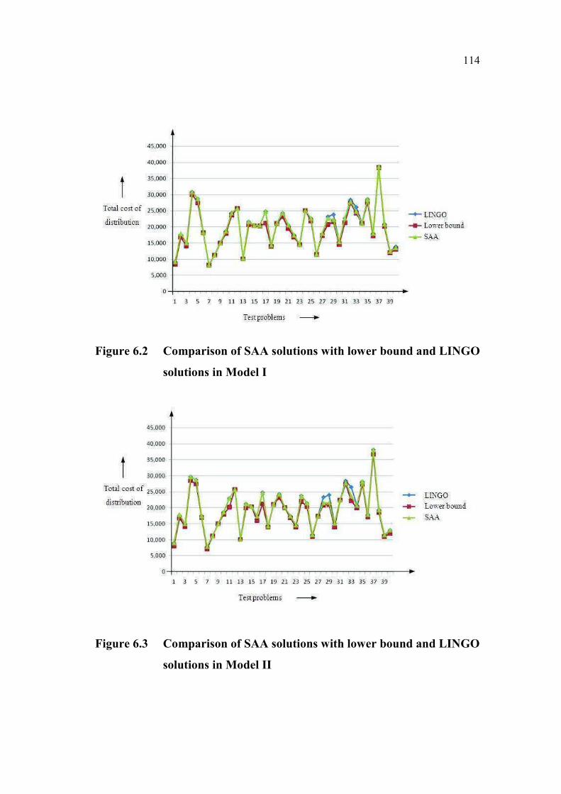
Figure 6.2 Comparison of SAA solutions with lower bound and LINGO
solutions in Model I
Figure 6.3 Comparison of SAA solutions with lower bound and LINGO
solutions in Model II
115
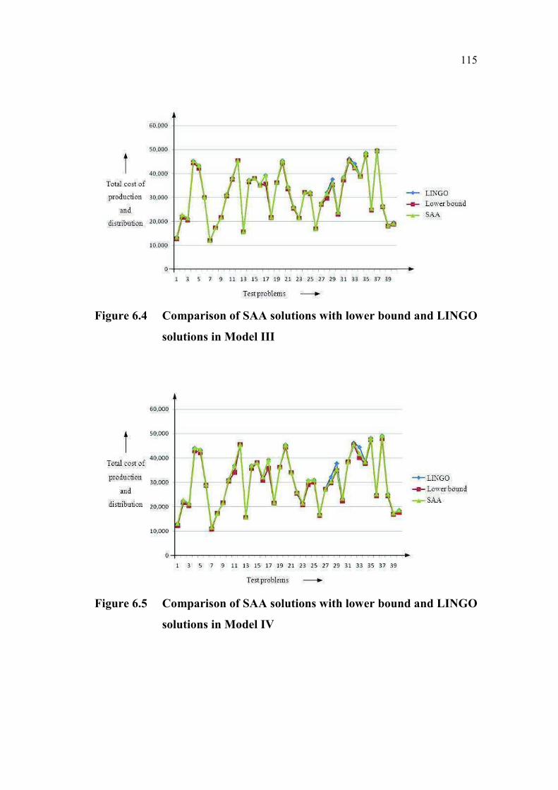
Figure 6.4 Comparison of SAA solutions with lower bound and LINGO
solutions in Model III
Figure 6.5 Comparison of SAA solutions with lower bound and LINGO
solutions in Model IV
116
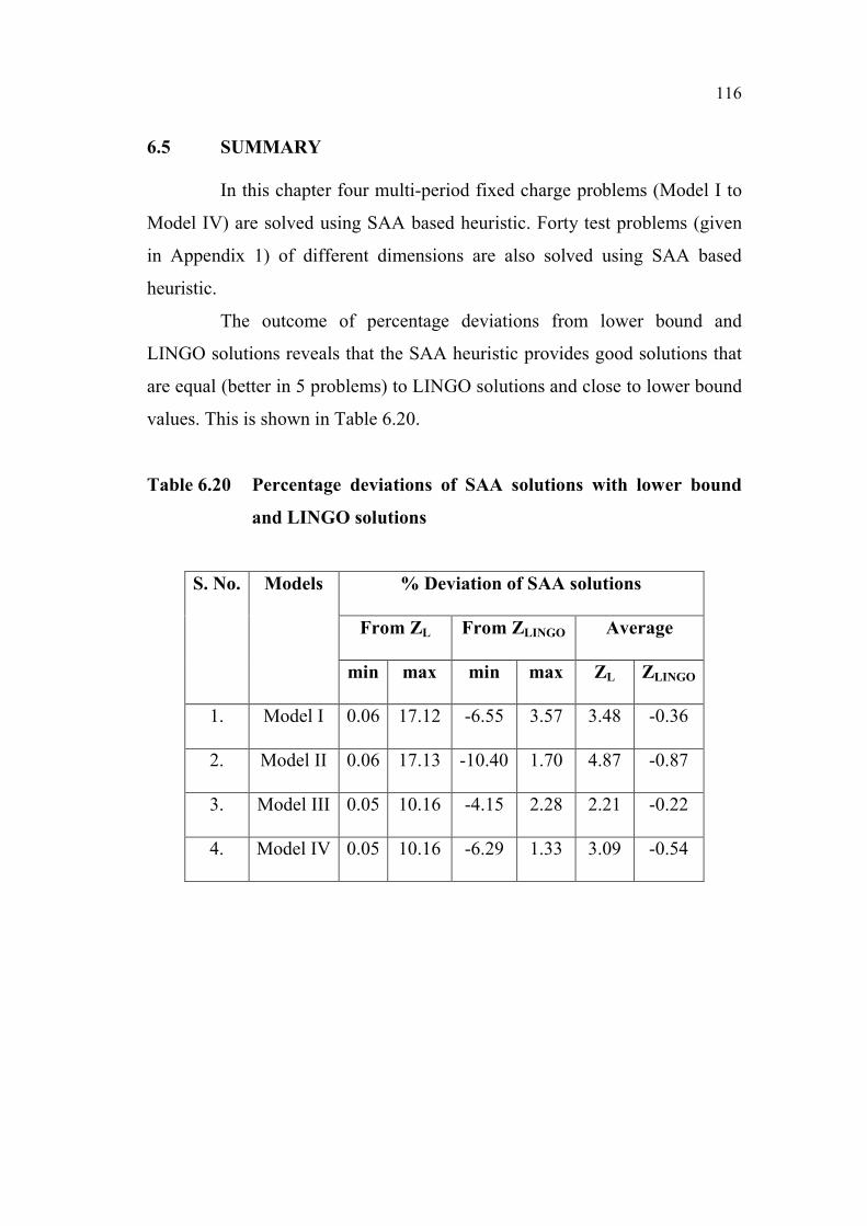
6.5 SUMMARY
In this chapter four multi-period fixed charge problems (Model I to
Model IV) are solved using SAA based heuristic. Forty test problems (given
in Appendix 1) of different dimensions are also solved using SAA based
heuristic.
The outcome of percentage deviations from lower bound and
LINGO solutions reveals that the SAA heuristic provides good solutions that
are equal (better in 5 problems) to LINGO solutions and close to lower bound
values. This is shown in Table 6.20.
Table 6.20 Percentage deviations of SAA solutions with lower bound
and LINGO solutions
S. No. Models % Deviation of SAA solutions
From ZL From ZLINGO Average
min max min max ZL ZLINGO
1. Model I 0.06 17.12 -6.55 3.57 3.48 -0.36
2. Model II 0.06 17.13 -10.40 1.70 4.87 -0.87
3. Model III 0.05 10.16 -4.15 2.28 2.21 -0.22
4. Model IV 0.05 10.16 -6.29 1.33 3.09 -0.54
117
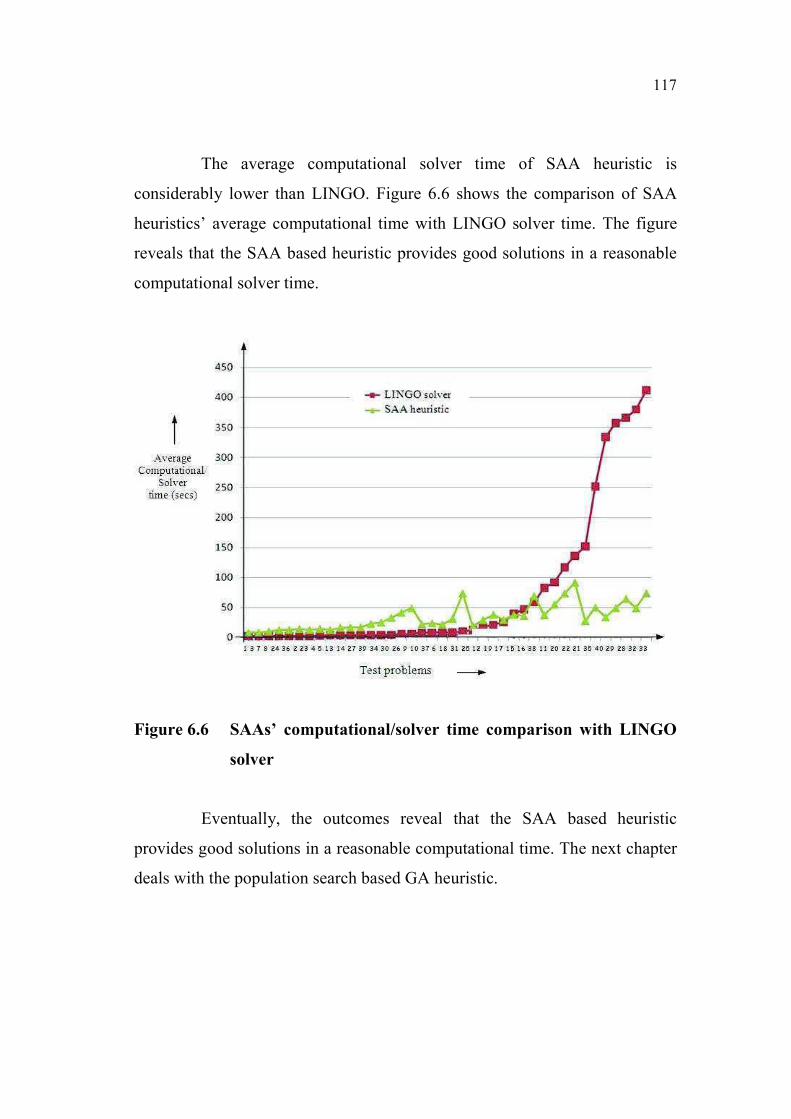
The average computational solver time of SAA heuristic is
considerably lower than LINGO. Figure 6.6 shows the comparison of SAA
heuristics’ average computational time with LINGO solver time. The figure
reveals that the SAA based heuristic provides good solutions in a reasonable
computational solver time.
Figure 6.6 SAAs� computational/solver time comparison with LINGO
solver
Eventually, the outcomes reveal that the SAA based heuristic
provides good solutions in a reasonable computational time. The next chapter
deals with the population search based GA heuristic.