chapter 6: point estimationmath.uhcl.edu/li/teach/s4345/ch6.pdf · 1 chapter 6: point estimation...

1

Chapter 6: Point Estimation

6.1 Descriptive Statistics

6.2 Exploratory Data Analysis

6.3 Order Statistics

6.4 Maximum Likelihood Estimation & Method of Moments Estimation

6.5 A Simple Regression Problem

6.6 Asymptotic Distributions of Maximum Likelihood Estimators

6.7 Sufficient Statistics

6.8 Bayesian Estimation – might be skipped

STAT 4345 Dr. Yingfu (Frank) Li6-1

What Is Statistics?

The word statistics has two meanings numerical facts: numbers

the field or discipline of study: the science of learning from data.

Types of Statistics Descriptive Statistics

Inferential Statistics It consists of methods that use sample results to help make decisions or

predictions about a population

Key idea of statistics From “part” to “whole”: use sample data to draw conclusions

regarding population via probability theory and stat methodology.

Major components Estimation; comparison; modeling

We’ll touch all three components in this class


2

§6.1 Descriptive Statistics

Data (variable) types Quantitative – all possible values from one or more intervals

Discrete vs continuous

Qualitative – countable possible values Nominal vs ordinal

Organizing, displaying, and describing data by using tables, graphs, and summary measures Describe the data numerically and graphically

Get a rough idea of the problem

Descriptive statistics for qualitative data – easy Frequency table, bar chart, pie chart, …

Descriptive statistics for quantitative data Frequency table, histograms, polygon, summary statistics, …


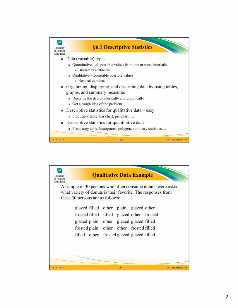
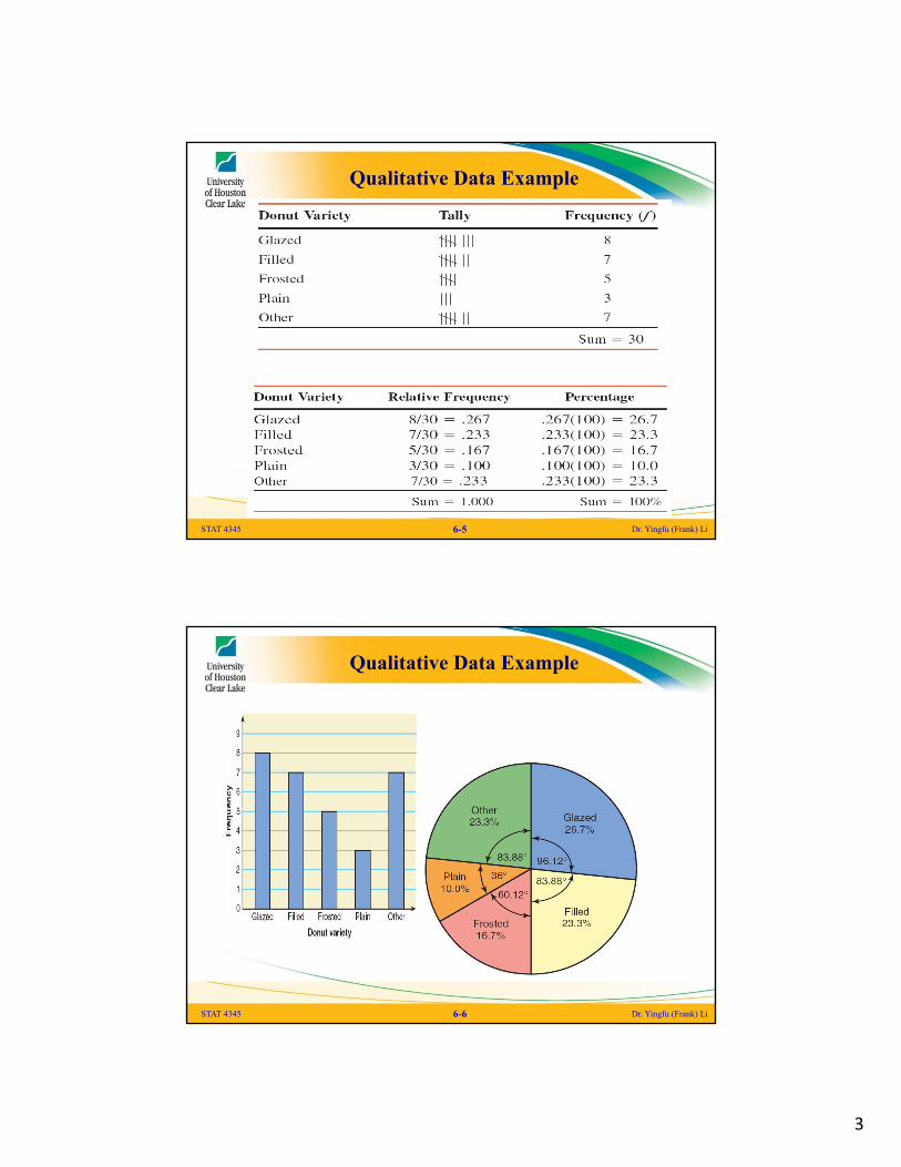
Qualitative Data Example

A sample of 30 persons who often consume donuts were asked what variety of donuts is their favorite. The responses from these 30 persons are as follows:

glazed filled other plain glazed other

frosted filled filled glazed other frosted

glazed plain other glazed glazed filled

frosted plain other other frosted filled

filled other frosted glazed glazed filled


3





4

Frequency Table for Quantitative Data

Group the data into classes, and These classes should cover the interval from the minimum to the maximum Common example – grade of a class

Steps to construct frequency table Range = largest value – smallest value

Pick the number of classes: usually 5 ~ 20

Class width: range / # of classes ≈ round up

Lower boundary of the first class

= smallest – half of smallest unit of data or place value The lowest boundary is below the smallest value and the highest

boundary is above the largest

Obtain all boundaries and these define classes

Construct (relative) frequency table

See book’s guideline at page 233


Terminology

Range = max – min of data values

Class – group

Class width = length of two boundaries of a class

Class intervals, class boundaries

Class limits - the smallest and the largest possible observed (recorded) values in a class

Class mark

A frequency table is constructed that lists the class intervals, the class limits, a tabulation of the measurements in the various classes, the frequency fi of each class, and the class marks.


5

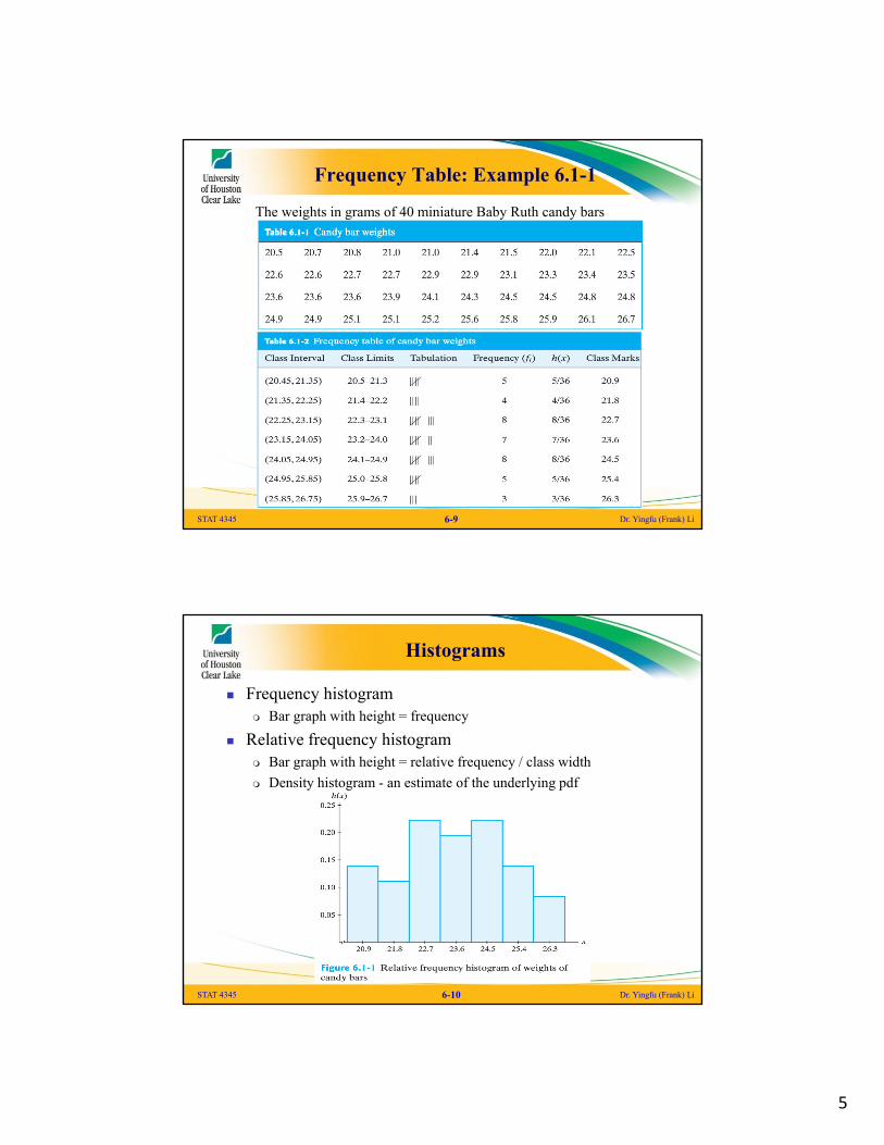
Frequency Table: Example 6.1-1

The weights in grams of 40 miniature Baby Ruth candy bars


Histograms

Frequency histogram Bar graph with height = frequency

Relative frequency histogram Bar graph with height = relative frequency / class width

Density histogram - an estimate of the underlying pdf


6

Numerical Descriptive Measures

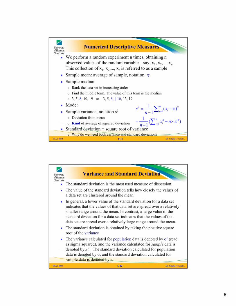
We perform a random experiment n times, obtaining n observed values of the random variable – say, x1, x2,..., xn. This collection of x1, x2,..., xn is referred to as a sample

Sample mean: average of sample, notation

Sample median Rank the data set in increasing order

Find the middle term. The value of this term is the median

3, 5, 8, 10, 19 or 3, 5, 8, || 10, 13, 19

Mode:

Sample variance, notation s2

Deviation from mean

Kind of average of squared deviation

Standard deviation = square root of variance Why do we need both variance and standard deviation?


x

2 2

1

2 2

1

1( )

11

( )1

n

ii

n

ii

s x xn

x n xn

Variance and Standard Deviation

The standard deviation is the most used measure of dispersion.

The value of the standard deviation tells how closely the values of a data set are clustered around the mean.

In general, a lower value of the standard deviation for a data set indicates that the values of that data set are spread over a relatively smaller range around the mean. In contrast, a large value of the standard deviation for a data set indicates that the values of that data set are spread over a relatively large range around the mean.

The standard deviation is obtained by taking the positive square root of the variance

The variance calculated for population data is denoted by σ² (read as sigma squared), and the variance calculated for sample data is denoted by s². The standard deviation calculated for population data is denoted by σ, and the standard deviation calculated for sample data is denoted by s.

Dr. Yingfu (Frank) Li6-12STAT 4345

7

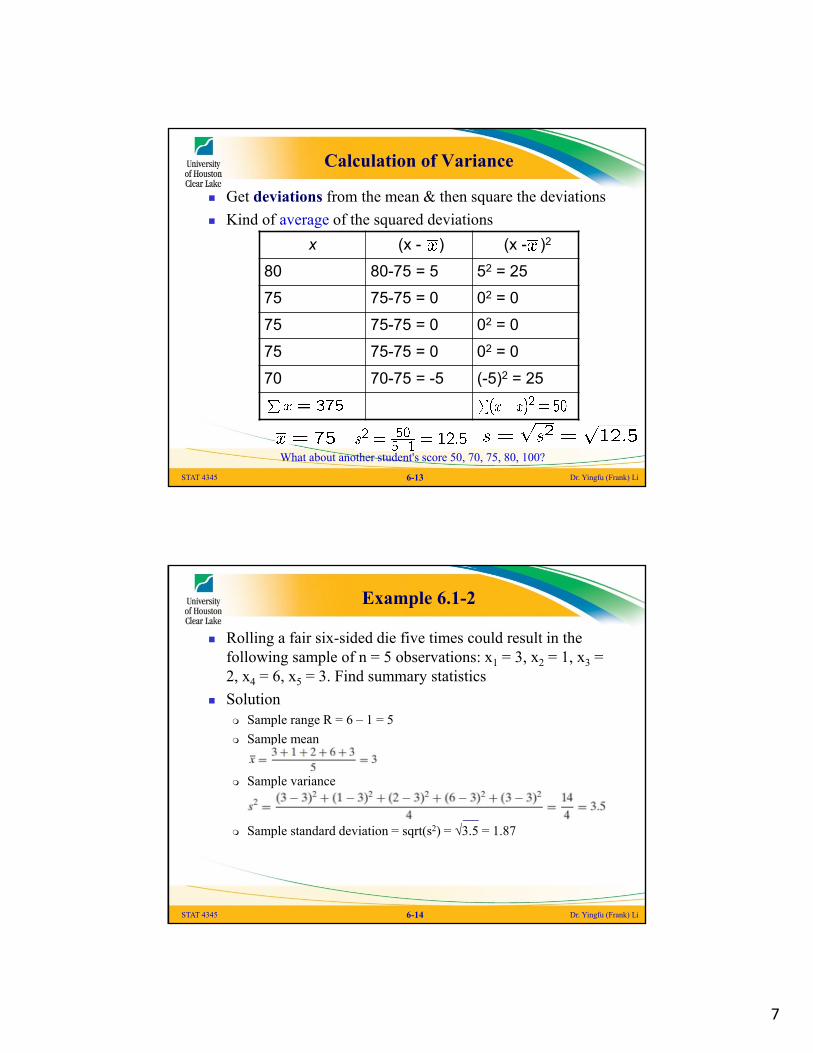
Calculation of Variance

Get deviations from the mean & then square the deviations

Kind of average of the squared deviations

Dr. Yingfu (Frank) Li6-13

x (x - ) (x - )2

80 80-75 = 5 52 = 25

75 75-75 = 0 02 = 0

75 75-75 = 0 02 = 0

75 75-75 = 0 02 = 0

70 70-75 = -5 (-5)2 = 25

STAT 4345

What about another student's score 50, 70, 75, 80, 100?

Example 6.1-2

Rolling a fair six-sided die five times could result in the following sample of n = 5 observations: x1 = 3, x2 = 1, x3 = 2, x4 = 6, x5 = 3. Find summary statistics

Solution Sample range R = 6 – 1 = 5

Sample mean

Sample variance

Sample standard deviation = sqrt(s2) = √3.5 = 1.87


8

Use of Standard Deviation - Empirical Rule

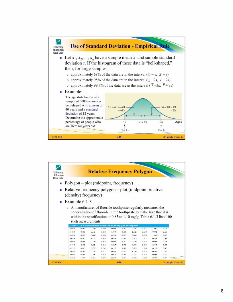
Let x1, x2, ..., xn have a sample mean and sample standard deviation s. If the histogram of these data is “bell-shaped,” then, for large samples, approximately 68% of the data are in the interval ( − s, + s)

approximately 95% of the data are in the interval ( −2s, + 2s)

approximately 99.7% of the data are in the interval ( −3s, + 3s)

Example:


x x

x xx x

The age distribution of a sample of 5000 persons is bell-shaped with a mean of 40 years and a standard deviation of 12 years. Determine the approximate percentage of people who are 16 to 64 years old.

x

Relative Frequency Polygon

Polygon – plot (midpoint, frequency)

Relative frequency polygon – plot (midpoint, relative (density) frequency)

Example 6.1-3 A manufacturer of fluoride toothpaste regularly measures the

concentration of fluoride in the toothpaste to make sure that it is within the specification of 0.85 to 1.10 mg/g. Table 6.1-3 lists 100 such measurements.


9

Relative Frequency Polygon


Histogram for Skewed Data

In some situations, it is not desirable to use class intervals of equal widths for frequency distribution and histogram. This is particularly true if the data are skewed with a very long tail.

It seems desirable to use class intervals of unequal lengths; thus, we cannot use the relative frequency polygon.

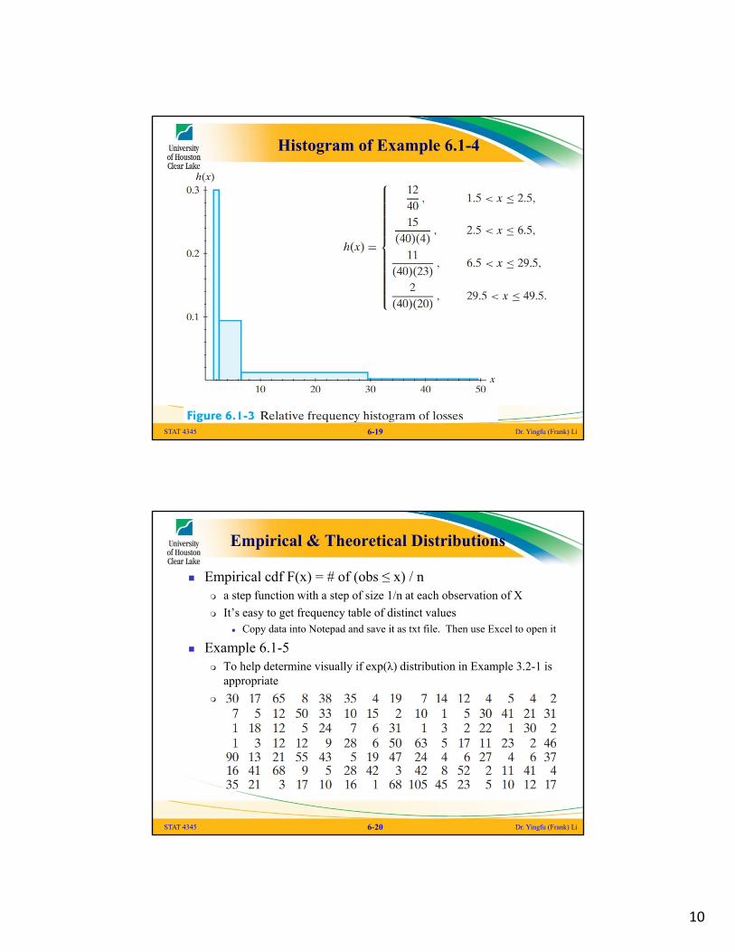
Example 6.1-4 The following 40 losses, due to wind-related catastrophes, were

recorded to the nearest $1 million (these data include only losses of $2 million or more): 2 2 2 2 2 2 2 2 2 2 2 2 3 3 3 3 4 4 4 5 5 5 5 6 6 6 6 8 8 9 15 17 22 23 24 24 25 27 32 43

The class boundaries are selected as c0 = 1.5, c1 = 2.5, c2 = 6.5, c3 = 29.5, and c4 = 49.5

The histogram needs to take unequal class width into consideration


10

Histogram of Example 6.1-4


Empirical & Theoretical Distributions

Empirical cdf F(x) = # of (obs ≤ x) / n a step function with a step of size 1/n at each observation of X

It’s easy to get frequency table of distinct values Copy data into Notepad and save it as txt file. Then use Excel to open it

Example 6.1-5 To help determine visually if exp(λ) distribution in Example 3.2-1 is

appropriate

Data set


11

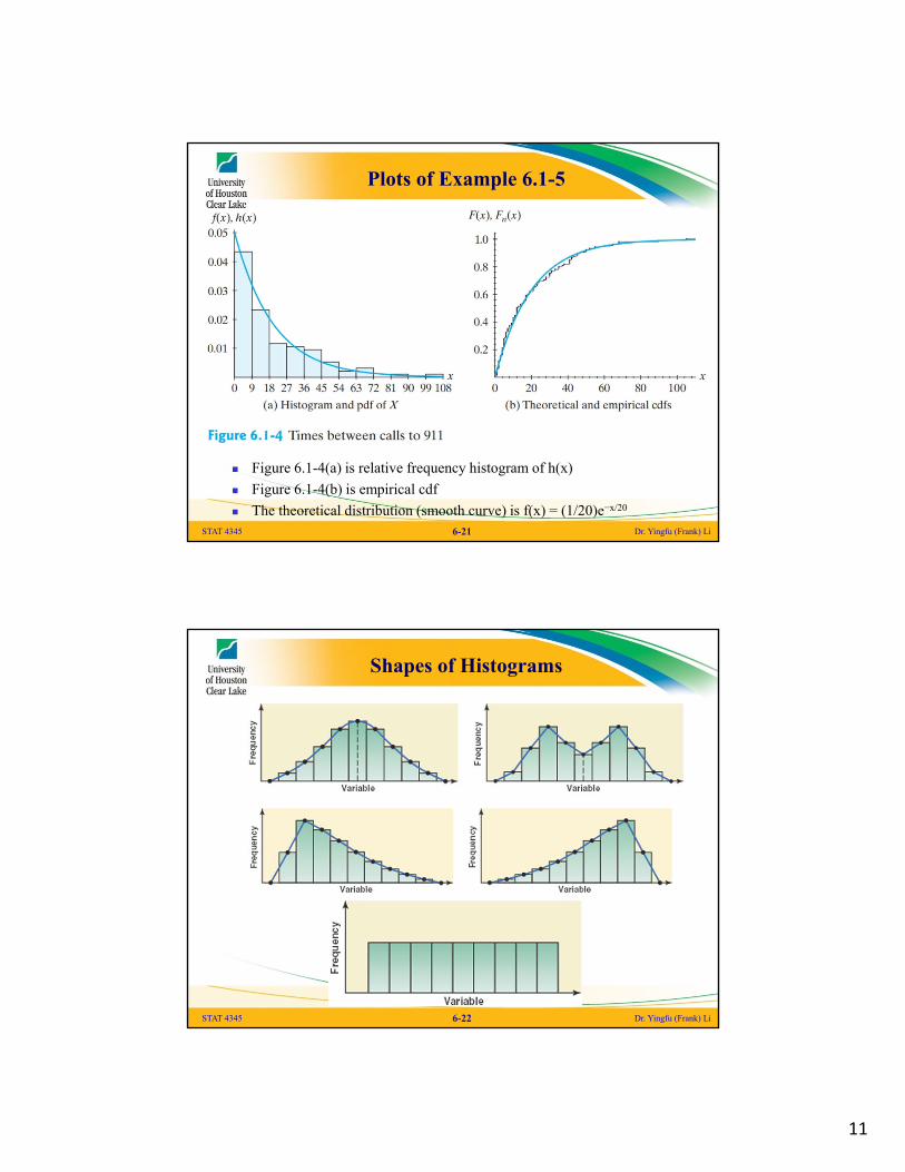
Plots of Example 6.1-5

Figure 6.1-4(a) is relative frequency histogram of h(x)

Figure 6.1-4(b) is empirical cdf

The theoretical distribution (smooth curve) is f(x) = (1/20)e−x/20


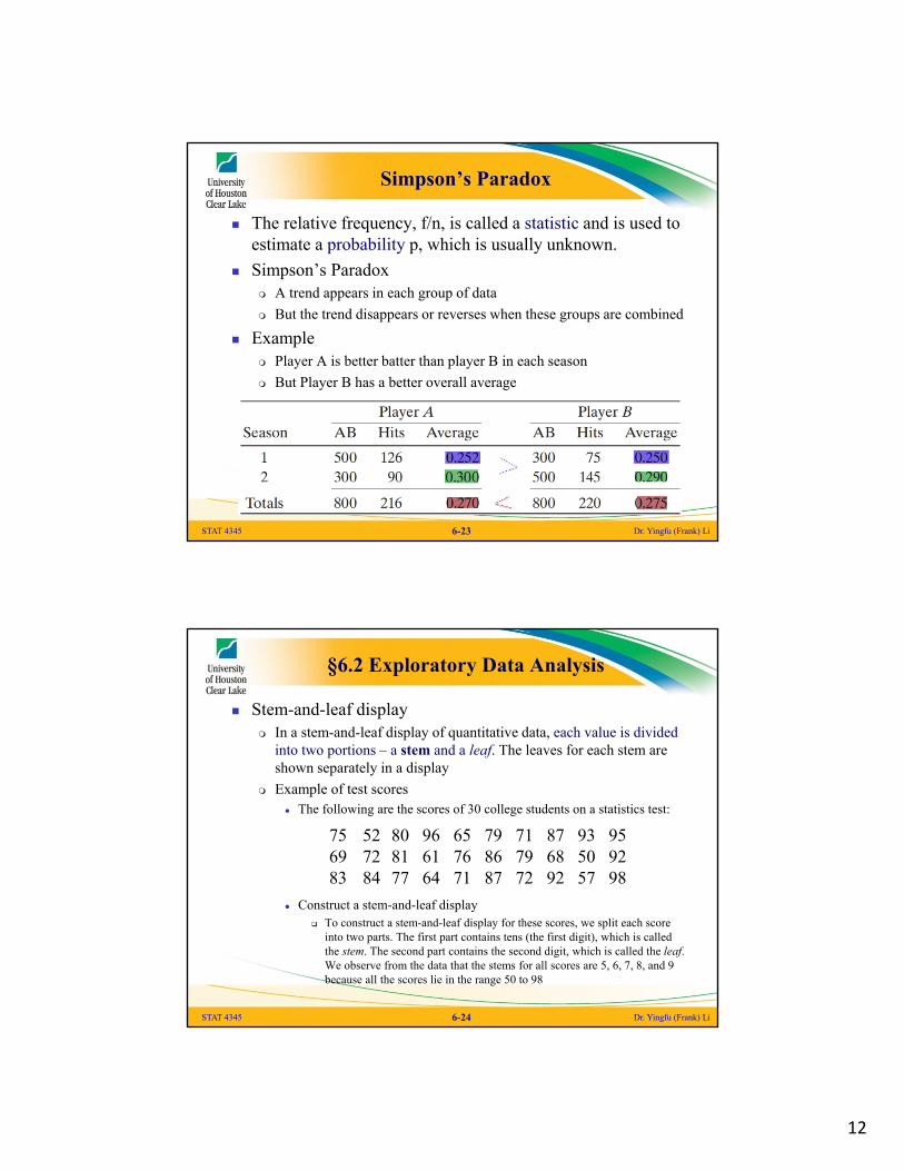
Shapes of Histograms


12

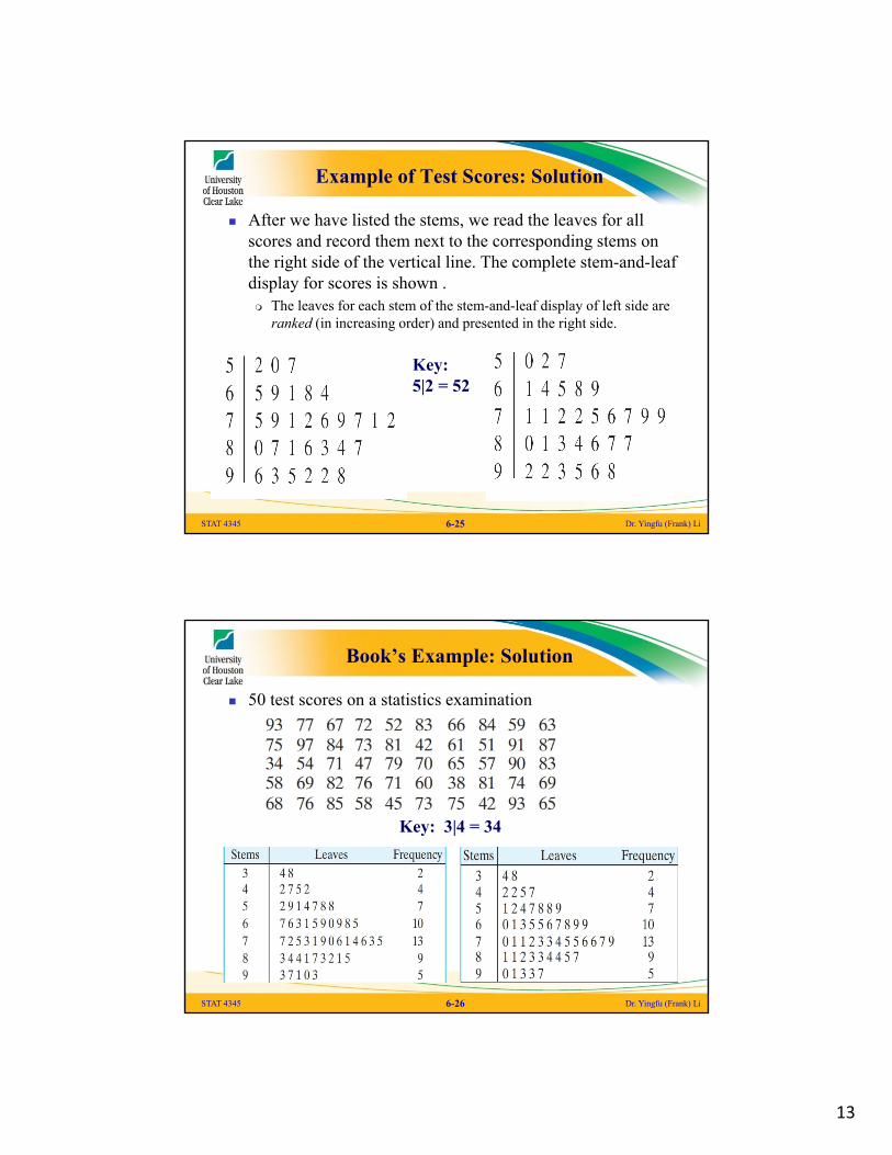
Simpson’s Paradox

The relative frequency, f/n, is called a statistic and is used to estimate a probability p, which is usually unknown.

Simpson’s Paradox A trend appears in each group of data

But the trend disappears or reverses when these groups are combined

Example Player A is better batter than player B in each season

But Player B has a better overall average


§6.2 Exploratory Data Analysis

Stem-and-leaf display In a stem-and-leaf display of quantitative data, each value is divided

into two portions – a stem and a leaf. The leaves for each stem are shown separately in a display

Example of test scores The following are the scores of 30 college students on a statistics test:

Construct a stem-and-leaf display To construct a stem-and-leaf display for these scores, we split each score

into two parts. The first part contains tens (the first digit), which is called the stem. The second part contains the second digit, which is called the leaf. We observe from the data that the stems for all scores are 5, 6, 7, 8, and 9 because all the scores lie in the range 50 to 98


756983

527284

808177

966164

657671

798687

717972

876892

935057

959298

13

Example of Test Scores: Solution

After we have listed the stems, we read the leaves for all scores and record them next to the corresponding stems on the right side of the vertical line. The complete stem-and-leaf display for scores is shown . The leaves for each stem of the stem-and-leaf display of left side are

ranked (in increasing order) and presented in the right side.

Dr. Yingfu (Frank) Li6-25

Key:5|2 = 52

STAT 4345

Book’s Example: Solution

50 test scores on a statistics examination


Key: 3|4 = 34

14

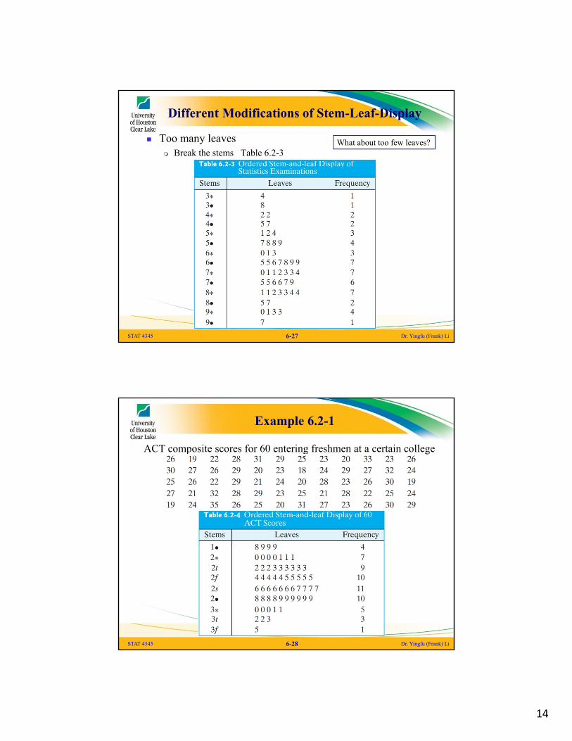
Different Modifications of Stem-Leaf-Display

Too many leaves Break the stems Table 6.2-3


What about too few leaves?

Example 6.2-1

ACT composite scores for 60 entering freshmen at a certain college


15

Measures of Position

Quartiles: Q1, Q2, Q3 Divide the ranked data into four equal parts

Interquartile range = Q3 – Q1

Box-and-Whisker Plot

Percentile: P1, P2, …, P99 Divide the ranked data into 100 equal parts

Q1 = P25, Q2 = P50 = median, Q3 = P75

Deciles = tens percentiles

(100p)th sample percentiles

where (n+1)p = r + a/b and r, a, & b are integers

Example 6.2-2 20th, 25th, 50th, 75th, 90th percentiles

Manual and computer waysSTAT 4345 Dr. Yingfu (Frank) Li6-29

Table 6.2-6 at page 250

Box-and-Whisker Plot


Five-Number Summary Min, Q1, Q2=Median, Q3, Max

Examples 6.2-3 & 6.2-4 – easy job!

A plot that shows the center, spread, and skewness of a data set. It is constructed by drawing a box and two whiskers that use the median, the first quartile, the third quartile, and the smallest and the largest values in the data set between the lower and the upper inner fences.

Formal BW plot Also used to detect potential outliers

Box = Q1, Q2, Q3

Whisker Inner fences: 1.5 times of IQR away from Q1(Q3)

Outer fences: 3 times of IQR away from Q1(Q3)

16

Examples 6.2-4 – 6.2-5

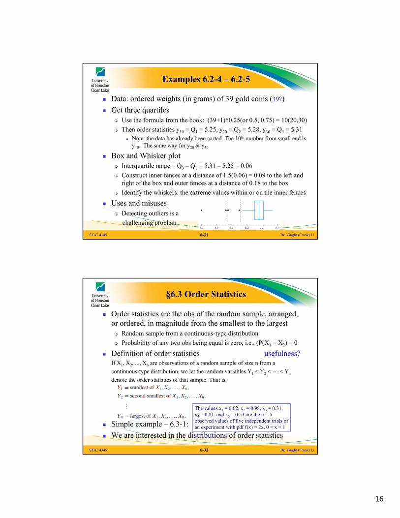
Data: ordered weights (in grams) of 39 gold coins (39?)

Get three quartiles Use the formula from the book: (39+1)*0.25(or 0.5, 0.75) = 10(20,30)

Then order statistics y10 = Q1 = 5.25, y20 = Q2 = 5.28, y30 = Q3 = 5.31 Note: the data has already been sorted. The 10th number from small end is

y10. The same way for y20 & y30

Box and Whisker plot Interquartile range = Q3 – Q1 = 5.31 – 5.25 = 0.06

Construct inner fences at a distance of 1.5(0.06) = 0.09 to the left and right of the box and outer fences at a distance of 0.18 to the box

Identify the whiskers: the extreme values within or on the inner fences

Uses and misuses Detecting outliers is a

challenging problem


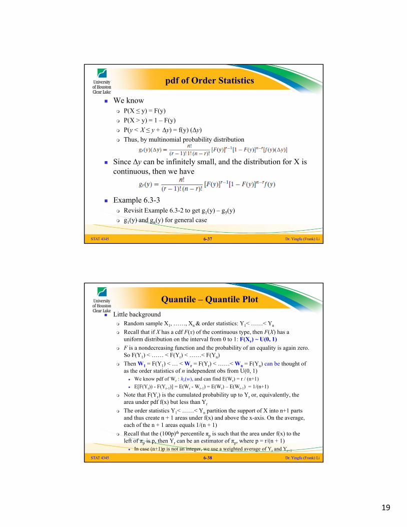
§6.3 Order Statistics

Order statistics are the obs of the random sample, arranged, or ordered, in magnitude from the smallest to the largest Random sample from a continuous-type distribution

Probability of any two obs being equal is zero, i.e., (P(X1 = X2) = 0

Definition of order statistics usefulness?If X1, X2, ..., Xn are observations of a random sample of size n from a

continuous-type distribution, we let the random variables Y1 < Y2 < ꞏꞏꞏ < Yn

denote the order statistics of that sample. That is,

Simple example – 6.3-1:

We are interested in the distributions of order statistics


The values x1 = 0.62, x2 = 0.98, x3 = 0.31, x4 = 0.81, and x5 = 0.53 are the n = 5 observed values of five independent trials of an experiment with pdf f(x) = 2x, 0 < x < 1

17

Recall Binomial Distribution

A Bernoulli experiment is a random experiment and it has only two mutually exclusive and exhaustive outcomes

Binomial Experiment is a pre-set number of Bernoulli trials 1. A Bernoulli ( success– failure) experiment is performed n times.

2. The trials are independent.

3. The probability of success on each trial is a constant p; then the probability of failure is q = 1 - p.

4. The random variable X = the number of successes in the n trials.

X has a Binomial distribution

General formula for Binomial distribution

Example: randomly guess answers for a 5-question multiple choices quiz

What about multinomial distribution?STAT 4345 Dr. Yingfu (Frank) Li6-33

1, 2, ...,( ) (1 ) ,x n x nf x nCx p p x

Example 6.3-2

Let Y1<Y2<Y3<Y4<Y5 be the order statistics associated with n independent observations X1, X2, X3, X4, X5, each from the distribution with pdf f(x) = 2x, 0 < x < 1. P(Y4 < 1/2) = ?

What do we mean by Y4 < 1/2? Random sample is X1, X2, X3, X4, X5, and random sample means…...

At least four of the random variables X1, X2, X3, X4, X5 must be less than ½. Think about it, what if only three of them < ½ and other two ≥ ½?

Can all five of them < ½?

Four or five of them < ½, but which 4 or 5?

Think about binomial distribution

P(Y4 < 1/2) = P(4 of {Xi}< 1/2) + P(5 of {Xi}< 1/2)


Treat {Xi < 1/2} as “success”

18

Distribution of Order Statistics

Just find P(Y4 < 1/2) = 0.0156.

What about a general case for 0 < y < 1, P(Y4 < y) = G(y) = ? Same argument: G(y) = P(Y4 < y) = P(4 of {Xi}< y) + P(5 of {Xi}< y)

Can we generalize it to any random sample’s order statistics? Random sample: X1, X2, ……, Xn ~ F(x)

Order statistics: Y1< …… < Yr< ……<Yn

Gr(y) = P(Yr < y) = ? Yr < y if and only if at least r of the n obs are less than or equal to y


Find the pdf gr(y)

pdf of Order Statistics

pdf in Example 6.3-2: g(y) =

pdf in general case:

Another heuristic way to pdf of order statistics To do this, we must recall the multinomial probability distribution

Imagine on a number line, yr belongs a very tiny interval (y, y+∆y]

P(y < Yr ≤ y + ∆y) ≈ gr(y)(∆y) = the probability that (r−1) items fall less than y, that (n−r) items are greater than y, and that one item falls between y and y + ∆y


P(X < y) P(X > y)y

y + ∆y

P(y < Yr ≤ y + ∆y)

# of possible orderings:

19

pdf of Order Statistics

We know P(X ≤ y) = F(y)

P(X > y) = 1 – F(y)

P(y < X ≤ y + ∆y) = f(y) (∆y)

Thus, by multinomial probability distribution

Since ∆y can be infinitely small, and the distribution for X is continuous, then we have

Example 6.3-3 Revisit Example 6.3-2 to get g1(y) – g5(y)

g1(y) and gn(y) for general case


Quantile – Quantile Plot

Little background Random sample X1, ……, Xn & order statistics: Y1< ……< Yn

Recall that if X has a cdf F(x) of the continuous type, then F(X) has a uniform distribution on the interval from 0 to 1: F(Xr) ~ U(0, 1)

F is a nondecreasing function and the probability of an equality is again zero. So F(Y1) < …… < F(Yr) < ……< F(Yn)

Then W1 = F(Y1) < … < Wr = F(Yr) < ……< Wn = F(Yn) can be thought of as the order statistics of n independent obs from U(0, 1) We know pdf of Wr : hr(w), and can find E(Wr) = r / (n+1)

E[F(Yr)) - F(Yr-1)] = E(Wr - Wr-1) = E(Wr) – E(Wr-1) = 1/(n+1)

Note that F(Yr) is the cumulated probability up to Yr or, equivalently, the area under pdf f(x) but less than Yr

The order statistics Y1< ……< Yn partition the support of X into n+1 parts and thus create n + 1 areas under f(x) and above the x-axis. On the average, each of the n + 1 areas equals 1/(n + 1)

Recall that the (100p)th percentile πp is such that the area under f(x) to the left of πp is p, then Yr can be an estimator of πp, where p = r/(n + 1) In case (n+1)p is not an integer, we use a weighted average of Yr and Yr+1


20

Quantile – Quantile Plot

General idea The (100p)th percentile of a distribution is often called the quantile of

order p.

yr is called the sample quantile of order r/(n+1)

Percentile πp of a theoretical distribution is the quantile of order p.

If the observations are indeed from the theoretical distribution, then yr ≈ πp. In other words, if we plot (yr, πp), a straight line through the origin with slope equal to 1 indicates that these observations are from the distribution

This plot is called quantile – quantile plot or, the q – q plot

q – q plot can be used to check any distributions

q – q plot for normal distribution yr ≈ πp = μ + σ zp

Plot of (yr, zp) is a straight line

Example 6.3-4 – using ExcelSTAT 4345 Dr. Yingfu (Frank) Li6-39

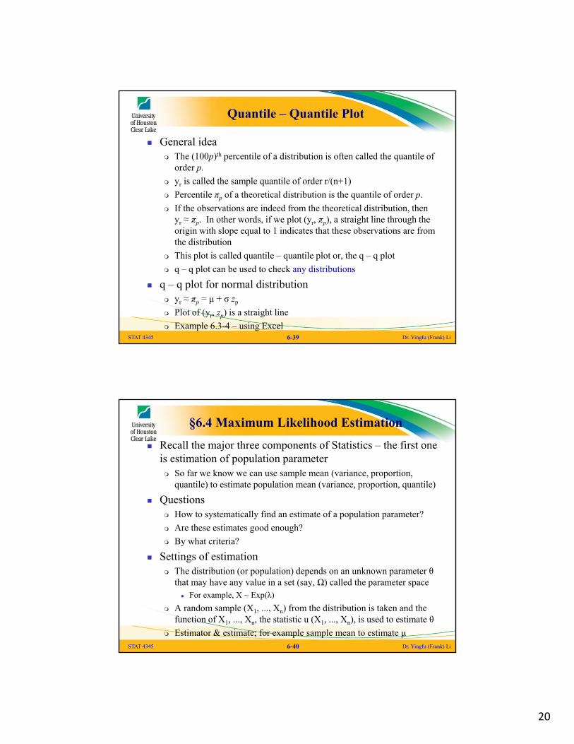
§6.4 Maximum Likelihood Estimation

Recall the major three components of Statistics – the first one is estimation of population parameter So far we know we can use sample mean (variance, proportion,

quantile) to estimate population mean (variance, proportion, quantile)

Questions How to systematically find an estimate of a population parameter?

Are these estimates good enough?

By what criteria?

Settings of estimation The distribution (or population) depends on an unknown parameter θ

that may have any value in a set (say, Ω) called the parameter space For example, X ~ Exp(λ)

A random sample (X1, ..., Xn) from the distribution is taken and the function of X1, ..., Xn, the statistic u (X1, ..., Xn), is used to estimate θ

Estimator & estimate; for example sample mean to estimate μSTAT 4345 Dr. Yingfu (Frank) Li6-40

21

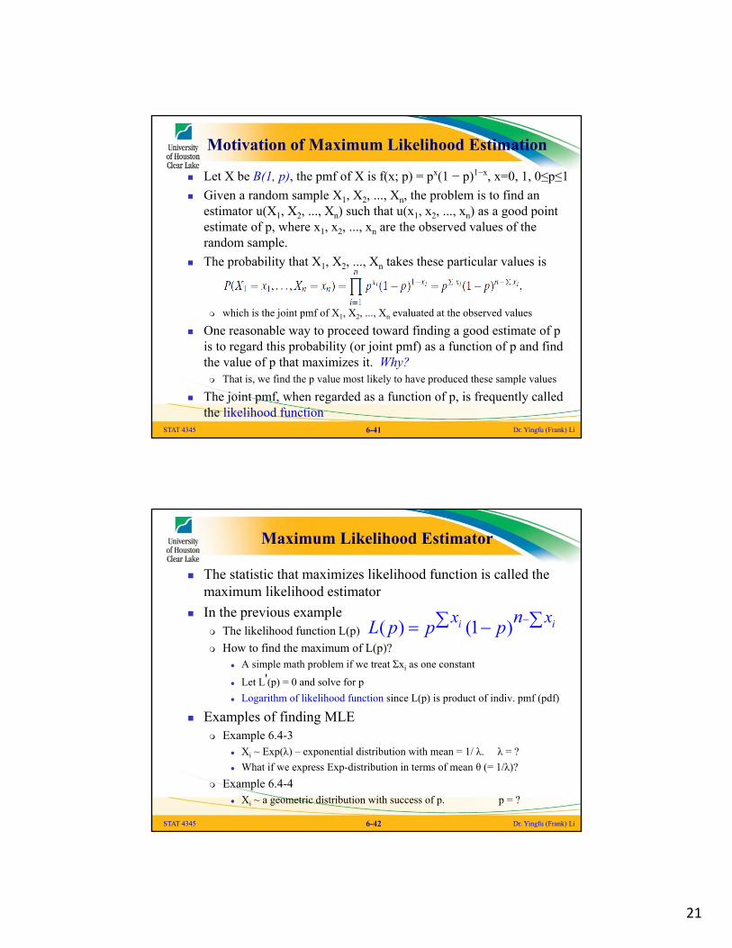
Motivation of Maximum Likelihood Estimation

Let X be B(1, p), the pmf of X is f(x; p) = px(1 − p)1−x, x=0, 1, 0≤p≤1

Given a random sample X1, X2, ..., Xn, the problem is to find an estimator u(X1, X2, ..., Xn) such that u(x1, x2, ..., xn) as a good point estimate of p, where x1, x2, ..., xn are the observed values of the random sample.

The probability that X1, X2, ..., Xn takes these particular values is

which is the joint pmf of X1, X2, ..., Xn evaluated at the observed values

One reasonable way to proceed toward finding a good estimate of p is to regard this probability (or joint pmf) as a function of p and find the value of p that maximizes it. Why? That is, we find the p value most likely to have produced these sample values

The joint pmf, when regarded as a function of p, is frequently called the likelihood function


Maximum Likelihood Estimator

The statistic that maximizes likelihood function is called the maximum likelihood estimator

In the previous example The likelihood function L(p)

How to find the maximum of L(p)? A simple math problem if we treat Σxi as one constant

Let L'(p) = 0 and solve for p

Logarithm of likelihood function since L(p) is product of indiv. pmf (pdf)

Examples of finding MLE Example 6.4-3

Xi ~ Exp(λ) – exponential distribution with mean = 1/ λ. λ = ?

What if we express Exp-distribution in terms of mean θ (= 1/λ)?

Example 6.4-4 Xi ~ a geometric distribution with success of p. p = ?


( ) (1 )i ix xnL p p p

22

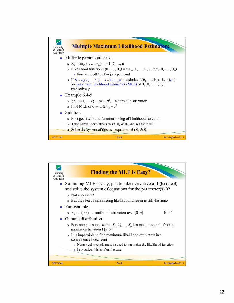
Multiple Maximum Likelihood Estimators

Multiple parameters case Xi ~ f(xi, θ1, …, θm), i = 1, 2, …, n

Likelihood function L(θ1, …, θm) = f(x1, θ1, …, θm)…f(xn, θ1, …, θm) Product of pdf / pmf or joint pdf / pmf

If maximize L(θ1, …, θm), then { } are maximum likelihood estimators (MLE) of θ1, θ2, . . . , θm, respectively

Example 6.4-5 {Xi , i=1, …, n} ~ N(µ, σ2) – a normal distribution

Find MLE of θ1 = µ & θ2 = σ2

Solution First get likelihood function => log of likelihood function

Take partial derivatives w.r.t. θ1 & θ2 and set them = 0

Solve the system of this two equations for θ1 & θ2


1( ,..., ), 1, 2,...,i i nX X i m

i

Finding the MLE is Easy?

So finding MLE is easy, just to take derivative of L(θ) or l(θ)and solve the system of equations for the parameter(s) θ? Not necessary!

But the idea of maximizing likelihood function is still the same

For example Xi ~ U(0,θ) – a uniform distribution over [0, θ]. θ = ?

Gamma distribution For example, suppose that X1, X2, ..., Xn is a random sample from a

gamma distribution Γ(α, λ)

It is impossible to find maximum likelihood estimators in a convenient closed form Numerical methods must be used to maximize the likelihood function.

In practice, this is often the case


23

Invariance Property of MLE

Theorem 6.4-1: If θ^ is the maximum likelihood estimator of θ based on a random sample from the distribution with pdf or pmf f(x; θ), and g is a one-to-one function, then g(θ^) is the maximum likelihood estimator of g(θ).

For example Xi ~ Exp(λ) – exponential distribution with mean = 1/ λ.

Find MLE of λ

What if we express Exp-distribution in terms of mean θ (= 1/λ)?

Again find MLE of θ

Compare the MLEs of λ and θ

New concept: unbiased estimator


Unbiased Estimator

If E[u(X1,X2,...,Xn)] = θ for all θ ∈ Ω, then the statistic u(X1,X2,...Xn) is called an unbiased estimator of θ. Otherwise, it is said to be biased

Examples Example 6.4-6: Let random sample X1, X2, X3, X4 from a uniform

distribution with pdf f(x; θ) = 1/θ, 0 < x ≤ θ Find MLE of θ – θ^ = max{X1, X2, X3, X4} = Y4

E(Y4) = 4θ/5 ≠ θ, biased estimator

Example 6.4-7: Random sample X1, X2, …, Xn from a normal distribution N(θ1=μ, θ2=σ2) We already know θ^

1 = μ^ = sample mean , θ^2 = (n – 1)S2 / n

It’s easy to show E(θ^1) = θ1 – unbiased

E(θ^2) = E[(n – 1)S2 / n] = (n – 1)σ2 / n ≠ θ2 = σ2 – biased


X

24

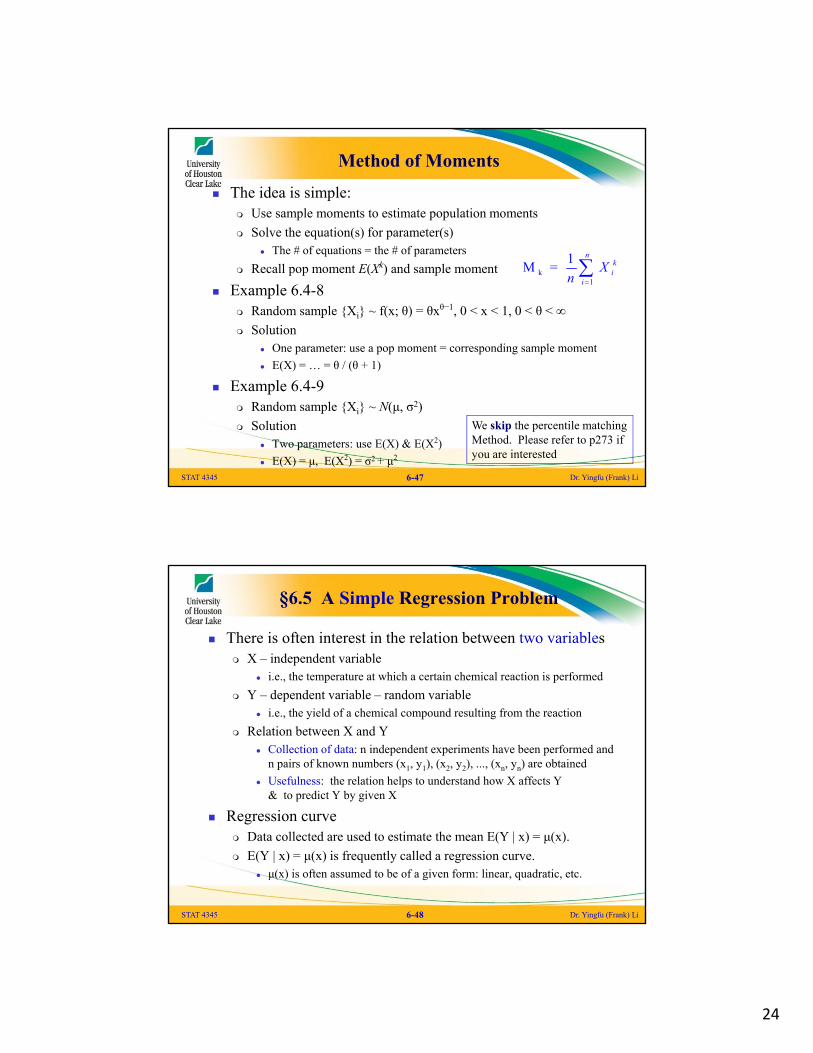
Method of Moments

The idea is simple: Use sample moments to estimate population moments

Solve the equation(s) for parameter(s) The # of equations = the # of parameters

Recall pop moment E(Xk) and sample moment

Example 6.4-8 Random sample {Xi} ~ f(x; θ) = θxθ−1, 0 < x < 1, 0 < θ < ∞

Solution One parameter: use a pop moment = corresponding sample moment

E(X) = … = θ / (θ + 1)

Example 6.4-9 Random sample {Xi} ~ N(μ, σ2)

Solution Two parameters: use E(X) & E(X2)

E(X) = μ, E(X2) = σ2 + μ2


k1

1M =

nki

i

Xn

We skip the percentile matchingMethod. Please refer to p273 if you are interested

§6.5 A Simple Regression Problem

There is often interest in the relation between two variables X – independent variable

i.e., the temperature at which a certain chemical reaction is performed

Y – dependent variable – random variable i.e., the yield of a chemical compound resulting from the reaction

Relation between X and Y Collection of data: n independent experiments have been performed and

n pairs of known numbers (x1, y1), (x2, y2), ..., (xn, yn) are obtained

Usefulness: the relation helps to understand how X affects Y & to predict Y by given X

Regression curve Data collected are used to estimate the mean E(Y | x) = μ(x).

E(Y | x) = μ(x) is frequently called a regression curve. μ(x) is often assumed to be of a given form: linear, quadratic, etc.


25

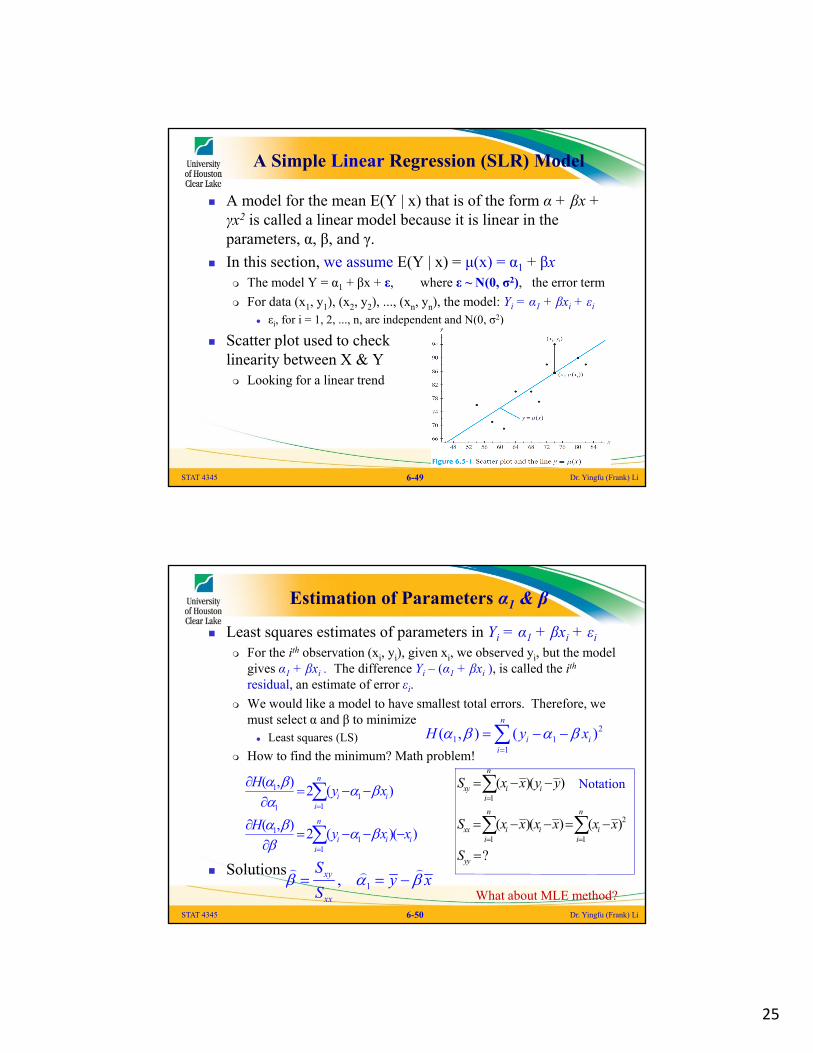
A Simple Linear Regression (SLR) Model

A model for the mean E(Y | x) that is of the form α + βx + γx2 is called a linear model because it is linear in the parameters, α, β, and γ.

In this section, we assume E(Y | x) = μ(x) = α1 + βx The model Y = α1 + βx + ε, where ε ~ N(0, σ2), the error term

For data (x1, y1), (x2, y2), ..., (xn, yn), the model: Yi = α1 + βxi + εi

εi, for i = 1, 2, ..., n, are independent and N(0, σ2)

Scatter plot used to check linearity between X & Y Looking for a linear trend


Estimation of Parameters α1 & β

Least squares estimates of parameters in Yi = α1 + βxi + εi

For the ith observation (xi, yi), given xi, we observed yi, but the model gives α1 + βxi . The difference Yi – (α1 + βxi ), is called the ith

residual, an estimate of error εi.

We would like a model to have smallest total errors. Therefore, we must select α and β to minimize Least squares (LS)

How to find the minimum? Math problem!

Solutions


21 1

1

( , ) ( )n

i ii

H y x

11

11

11

1

( , )2 ( )

( , )2 ( )( )

n

i ii

n

i i ii

Hy x

Hy x x

1

2

1 1

( )( )

( )( ) ( )

?

n

xy i ii

n n

xx i i ii i

yy

S x x y y

S x x x x x x

S

1, xy

xx

Sy x

S

Notation

What about MLE method?

26

Estimation of σ2 and α

We know εi, for i = 1, 2, ..., n, are independent and N(0, σ2)

ei is the observed value of εi, given xi

By MLE, the estimate of σ2

Centralized xi and then fit the model: Yi = α + β(xi – ) + εi

is the sample mean of {xi}

Better for finding MLE of parameters

Both estimates (from MLE & LS) are essentially the same.


2 2 21

1 1

1 1( )

n n

MLE i i ii i

e y xn n

x

1, xy

xx

Sy y x

S

x

Examples of SLR

Example 6.5-1 The data are 10 pairs of test scores of 10 students in a psychology

class, x being the score on a preliminary test and y the score on the final examination. Fit a simple linear regression model

Manual calculation & using Excel

More examples to show scatter plot Data exercise 11-65 from Applied Statistical Methods

Exercise 6.5-6


27

Finding the Distributions of Estiamted Parameters

Treat {x1, x2, ..., xn} as nonrandom constants and then {Yi} are random variables following normal distributions E(Yi) = α1 + βxi and Var(Yi) = σ2

Estimated parameters We can show E( ) = β

E( ) = α1

E( ) = α

Var( ) = σ2/ n

Var( ) =

We actually can show and follow normal distributions So we can make inference regarding these parameters


1

2

1

( )( )

( )

n

i ixy i

nxx

ii

x x y yS

S x x

1 y x

1

y

2 2

1

/ ( )n

ii

x x

§6.6 Asymptotic Distributions of Maximum Likelihood Estimators

Random sample Xi ~ f(xi, θ), i = 1, 2, …, n

MLE of θ

We can show the MLE of θ asymptotically follow normal distribution with mean θ and variance related to the information of random sample, i.e.

For multiple parameter version, we have a similar result.


1 2( , , ..., )nu X X X

2 2

2

2

(0,1)1/ { [ln ( , )] /

where I( ) = [ ln ( , )] is often called the Fisher information of ( , )

( ) ( ) (0,1)

NnE f X

E f X f X

nI N

28

Example 6.6-1 & Example 6.6-2

Example 6.6-1 Exponential pdf f(x; θ) = e–x/θ / θ, 0 < x < ∞, 0 < θ < ∞

MLE for θ is sample mean

We show that has an approximate normal distribution By MLE asymptotical normality

By CLT

Example 6.6-2 Poisson distribution f(x; λ) = λx e–λ / x!, x = 0, 1, …; 0 < λ < ∞

MLE for λ is sample mean

We show that has an approximate normal distribution By MLE asymptotical normality

By CLT


XX

XX

§6.7 Sufficient Statistics

What is a sufficient statistic (SS) and why do we need it?

A sufficient statistic for θ contains all information regarding θ

Examples of finding sufficient statistic Example 6.7-1: X1, X2, ..., Xn ~ Poisson(λ)

Example 6.7-2: X1, X2, ..., Xn ~ N(μ, 1)

Example 6.7-3: X1, X2, ..., Xn ~ B(1, p) – Bernoulli distribution


29

Important Properties of Sufficient Statistic

The conditional probability of any given event A in the support of X1, X2, ..., Xn, given that sufficient stat Y = y, does not depend on θ. see Example 6.7-3

If there is a sufficient statistic for the parameter under consideration and if the maximum likelihood estimator of this parameter is unique, then the maximum likelihood estimator is a function of the sufficient statistic. If a sufficient statistic exists, then the likelihood function is

Maximize L(θ) = maximize ϕ[u(x1, x2, ..., xn); θ]

θ must be a function of u(x1, x2, ..., xn)

MLE of θ is a function of the sufficient statistic u(x1, x2, ..., xn)


Another Way to Find Sufficient Statistic

Theorem 6.7-1

Examples Example 6.7-4: X1, X2, ..., Xn ~ Exp(λ = 1/θ), find SS for θ

Example 6.7-1: X1, X2, ..., Xn ~ Poisson(λ)

Example 6.7-2: X1, X2, ..., Xn ~ N(μ, 1)


30

Jointly Sufficient Statistics for Multiple Parameters

In many cases, we have two (or more) parameters—say, θ1

and θ2. All of the preceding concepts can be extended to these situations.

If , where ϕ depends on x1, x2, ..., xn only via u1(x1, x2, ..., xn), u2(x1, x2, ..., xn), and h(x1, x2, ..., xn) does not depend upon θ1

or θ2, then Y1 = u1(X1, X2, ..., Xn) and Y2 = u2(X1, X2, ..., Xn)are jointly sufficient statistics for θ1 and θ2. Can be further generalized to three or more parameters.

Example 6.7-5 X1, X2, ..., Xn ~ N(θ1 = μ, θ2 = σ2), find the jointly sufficient stat

Relation to MLEs


Importance of Sufficient Statistic

The important point to stress for cases in which sufficient statistics exist is that once the sufficient statistics are given, there is no additional information about the parameters left in the remaining (conditional) distribution. That is, all statistical inferences should be based upon the sufficient statistics.

Theorem 6.7-2 – Rao–Blackwell theorem

Provide a way to find a (uniformly minimum variance unbiased estimator (UMVUE), which is out of scope of this class.


chapter 6: point estimationmath.uhcl.edu/li/teach/s4345/ch6.pdf · 1 chapter 6: point estimation...

Documents