chapter 6 partial load in a specific area of the slab. define the load and left click inside the...
TRANSCRIPT

CHAPTER 6 «LOADS»
2
CONTENTS
I. THE NEW UPGRADED INTERFAFE OF SCADA Pro 3
II. DETAILED DESCRIPTION OF THE NEW INTERFACE 4
1. LOADS 4
1.1 Definition 4
1.2 Slab Loads 7
1.3 Member Load 12
1.4 Wind and Snow Loads 28

CHAPTER 6 «LOADS»
3
I. THE NEW UPGRADED INTERFAFE OF SCADA Pro

CHAPTER 6 «LOADS»
4
II. DETAILED DESCRIPTION OF THE NEW INTERFACE In the new upgraded SCADA Pro all commands are grouped in 11 Units.
1. LOADS
6th Unite, is called “Loads” and includes the following 4 groups of commands:
1. Definition 2. Slab Loads 3. Member Loads 4. Wind and Snow Loads
1.1 Definition
“Definition” command group allows the definition of the loads and their corresponding groups.
Basic condition for loads application is the definition of the respective load cases. Each load
will belong to one of those cases.
To define the Load cases use “Load Cases” command. In the dialog box:
CHAPTER 6 «LOADS»
5
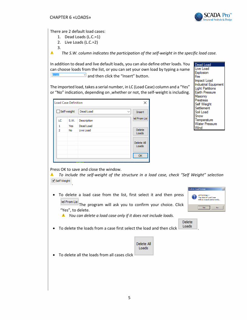
There are 2 default load cases: 1. Dead Loads (L.C.=1) 2. Live Loads (L.C.=2) 3.
The S.W. column indicates the participation of the self-weight in the specific load case. In addition to dead and live default loads, you can also define other loads. You can choose loads from the list, or you can set your own load by typing a name
and then click the “Insert” button. The imported load, takes a serial number, in LC (Load Case) column and a “Yes” or “No” indication, depending on ,whether or not, the self-weight is including.
Press OK to save and close the window. To include the self-weight of the structure in a load case, check “Self Weight” selection
.
To delete a load case from the list, first select it and then press
The program will ask you to confirm your choice. Click “Yes”, to delete.
You can delete a load case only if it does not include loads.
To delete the loads from a case first select the load and then click .
To delete all the loads from all cases click
CHAPTER 6 «LOADS»
6
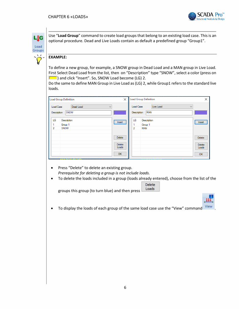
Use “Load Group” command to create load groups that belong to an existing load case. This is an optional procedure. Dead and Live Loads contain as default a predefined group “Group1”.
EXAMPLE: To define a new group, for example, a SNOW group in Dead Load and a MAN group in Live Load. First Select Dead Load from the list, then on “Description” type “SNOW”, select a color (press on
) and click “Insert”. So, SNOW Load become (LG) 2. Do the same to define MAN Group in Live Load as (LG) 2, while Group1 refers to the standard live loads.
Press “Delete” to delete an existing group. Prerequisite for deleting a group is not include loads.
To delete the loads included in a group (loads already entered), choose from the list of the
groups this group (to turn blue) and then press
To display the loads of each group of the same load case use the “View” command .
CHAPTER 6 «LOADS»
7
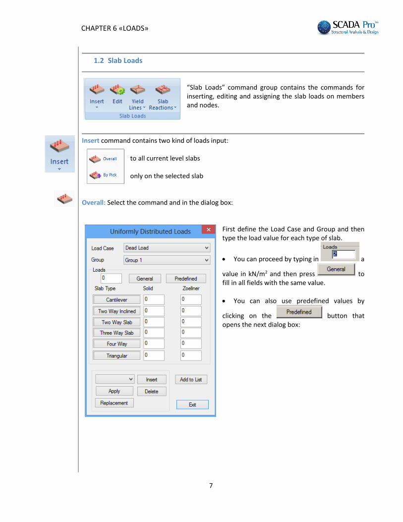
1.2 Slab Loads
“Slab Loads” command group contains the commands for inserting, editing and assigning the slab loads on members and nodes.
Insert command contains two kind of loads input:
to all current level slabs only on the selected slab
Overall: Select the command and in the dialog box:
First define the Load Case and Group and then type the load value for each type of slab.
You can proceed by typing in a
value in kN/m2 and then press to fill in all fields with the same value.
You can also use predefined values by
clicking on the button that opens the next dialog box:

CHAPTER 6 «LOADS»
8
Select from the “Import from” list the predefined load to define loads directly, or define your own load, by typing a “Description”, a value “Load (kN/m2)” and in case you want to save the load to the library click
the button .
Define the loads and press .
The load case and group are displayed in the list (Lc=1: Load Case 1/Lg=1: Group 1) automatically.
Follow the same procedure for the other load cases (ex. Live Load) and press ,
to display the Load case and group (Lc=2: Load Case 2/Lg=1: Group 1).
By selecting , all defined loads are applied to all current level slabs.
The loads’ assignment for the first time means that the loads in the list will be applied to all current level slabs.
But, in case of slabs containing existing loads, by clicking on the button, the existing loads will be replaced.
EXAMPLE 1: Suppose that you have already assigned loads in all current level slabs with dead and live loads.
- If you define a new value for the dead loads and press , the program will apply
the new dead load value and 0 live load (the list contains only dead load and no live load).
- But, if you want to replace dead loads and keep the existing live loads, then press
- Press to cancel an inserted load from the list.

CHAPTER 6 «LOADS»
9
EXAMPLE 2: Suppose that a dead load of 1 kN/m2 is already applied on a slab and you want to add another dead load 2 KN/m2.
Define the load and press .
Select command to confirm. You can also replace only the value of a specific Slab Type. Type the value in the corresponding
space and then click the type . This value will replace the first one to all slabs with the same type.
Press to close the dialog box without save, or press to save the changes.
By pick: select the command and then left click inside a slab. In the dialog box:
Define “Load Case”, “Load Group”, and type the value in KN/m2. Then select “Load Type”.
There are 3 “Load Types”:
Uniform Insert uniform loads over the entire surface of the slab. Define the load and left click inside the slab. • Partial Insert partial load in a specific area of the slab. Define the load and left click inside the slab. Then select a side to identify the direction and then left click to indicate a vertex and move mouse to describe the load area.

CHAPTER 6 «LOADS»
10
• Linear Insert linear load over the slab and follow the same procedure as in partial loads. To define the position of the load, left click to identify the two ends of the line (start and end point).
Partial and Linear loads will be replaced by an equivalent uniform load on the entire slab, regarding the attribution to the slab members
Define “Load” in kN/m2.
You can also use predefined values using button, as previous.
Press to close the dialog box and click inside one or more slabs’ area to apply the load.
To edit and modify slab loads use Edit command. Select the command and click inside a slab. In the dialog box:
Select Load Case and Group, then from the list select the load for editing.
Activate and all the loads will be deleted from the list. Otherwise, press
to delete only the selected load from the list.
Loads are not deleted immediately but first "Delete" is displayed on "Status" column, which
means “ready to delete”.
To delete them permanently, press .
command invalidate the previous action (cancels "Delete" designation in Status column)
Press to close the dialog box without saving, or to save the changes.
CHAPTER 6 «LOADS»
11
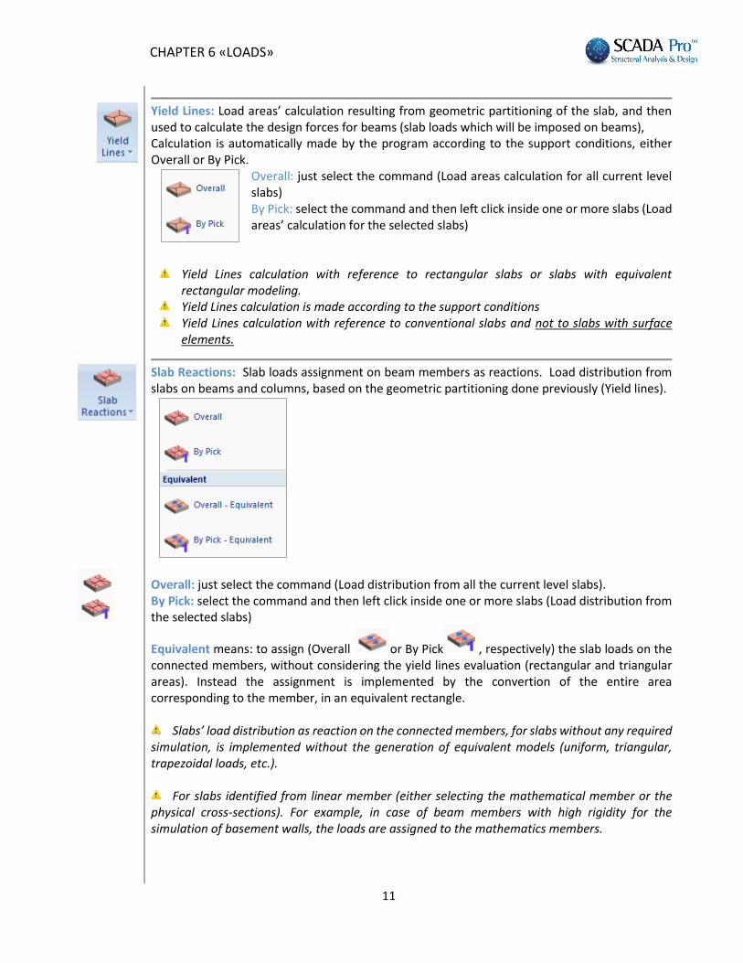
Yield Lines: Load areas’ calculation resulting from geometric partitioning of the slab, and then used to calculate the design forces for beams (slab loads which will be imposed on beams), Calculation is automatically made by the program according to the support conditions, either Overall or By Pick.
Overall: just select the command (Load areas calculation for all current level slabs) By Pick: select the command and then left click inside one or more slabs (Load areas’ calculation for the selected slabs)
Yield Lines calculation with reference to rectangular slabs or slabs with equivalent
rectangular modeling. Yield Lines calculation is made according to the support conditions Yield Lines calculation with reference to conventional slabs and not to slabs with surface
elements.
Slab Reactions: Slab loads assignment on beam members as reactions. Load distribution from slabs on beams and columns, based on the geometric partitioning done previously (Yield lines).
Overall: just select the command (Load distribution from all the current level slabs). By Pick: select the command and then left click inside one or more slabs (Load distribution from the selected slabs)
Equivalent means: to assign (Overall or By Pick , respectively) the slab loads on the connected members, without considering the yield lines evaluation (rectangular and triangular areas). Instead the assignment is implemented by the convertion of the entire area corresponding to the member, in an equivalent rectangle.
Slabs’ load distribution as reaction on the connected members, for slabs without any required simulation, is implemented without the generation of equivalent models (uniform, triangular, trapezoidal loads, etc.).
For slabs identified from linear member (either selecting the mathematical member or the physical cross-sections). For example, in case of beam members with high rigidity for the simulation of basement walls, the loads are assigned to the mathematics members.
CHAPTER 6 «LOADS»
12
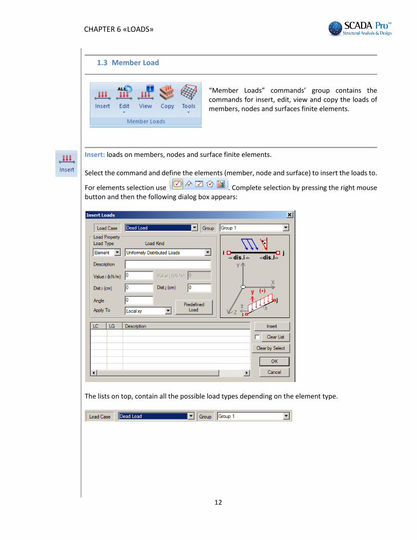
1.3 Member Load
“Member Loads” commands’ group contains the commands for insert, edit, view and copy the loads of members, nodes and surfaces finite elements.
Insert: loads on members, nodes and surface finite elements. Select the command and define the elements (member, node and surface) to insert the loads to.
For elements selection use . Complete selection by pressing the right mouse button and then the following dialog box appears:
The lists on top, contain all the possible load types depending on the element type.

CHAPTER 6 «LOADS»
13
“Load Property”:
Select the “Type” of the element and the “Type” of the load
. According to the element “Type” and the load “Type”, the “Load Property” is modified. Fill in the fields according to the drawing, type a description, the values and the corresponding distances.
Member Load Sign :
Loads’ sign convention is made versus the local coordinate system of each member, which is based on the rule of the “right hand”.
Specifically: 1. BEAMS : x-x is the local axes directed from the start to the end point (red vectors), y-y is the vertical axes (perpendicular to the local axis x-x) parallel to the height of the slab (green vector). It is always directed like Y Absolut axes (bottom-up). z-z is the third vertical axis, perpendicular to the plane defined by the xx and yy local axes (blue vector).

CHAPTER 6 «LOADS»
14
2. COLUMNS : x-x is the local axis directed from the start to the end point meaning bottom-up direction (red vectors), y-y is the vertical axis (perpendicular to the local x-x) directed like X Absolut axis (green vector). z-z is the third vertical axis, perpendicular to the plane defined by the xx and yy local axis (blue vector).
Beams and columns local axes can also be defined using the rule of the right hand with your thumb along the positive axis xx, point along the positive yy and the middle along the positive zz.
Nodes Load Sign :
Nodes’ loads are always directed according the Absolute X,Y,Z axes.
The next dialog box section, is the load list.
The list is filled in by defining the loads and selecting the “Insert” command.

CHAPTER 6 «LOADS»
15
Plate
EXAMPLE: Insert a uniform distributed load (U.D.F. Uniformly Distributed Force) that belongs to Load Case (LC) 1 (Dead Loads) and Load Group (LG) 1. The numbers after the description (Wall) are: start load value, end load value, the distance of the load from the beginning, the distance of load from the end and the angle.
By activating , all the loads of the list will be deleted. Otherwise, press
to delete only the selected load from the list.
Plate Loads
Allows you to define a Pressure, and also, added the possibility to enter Temperature Variations load for finite surface elements. More specifically, for Plate (shell) elements added Uniform Temperature Variations and Linear Temperature Variations loads.
- Uniform Temperature Variations causes membrane deformation in the plane of the element, while
- Linear Temperature Variations causes deflection.

CHAPTER 6 «LOADS»
16
NOTE:
To note that the two loads of the plate element can be integrated either on the same loading, or in two different loadings.
Integrating both loads at the same analysis scenario, you will get aggregated results in one load (the first).
Considering as two different loadings, to obtain individual results, each load MUST go to a different analysis scenario.
The procedure to follow is:
NOTE:
For Plane elements (Stress, Strain, Axisymmetric) only Uniform Temperature Variation is possible.

CHAPTER 6 «LOADS»
17
Edit: for editing the existing loads’ properties.
Overall: for editing existing loads’ properties on the current levels. Select the command and the dialog box opens:
In the load list you can see all the imported loads according to the selection. For example, select: Dead Load/Group 1/Element/ Uniformly Distributed Loads. The list describes all the existing loads according to the selection. (U.D.F. Uniformly Distributed Force, S.R. Slab reactions) When you choose a load, the values appear on the top of the window where you can modify them.
Press the command to save the changes.
By activating , all the loads on the list will be deleted. Otherwise, press
to delete only the selected loads. Loads are not deleted immediately but first the "Delete" indication is displayed on "Status" column, which means “ready to delete”. To delete them permanently, press
.

CHAPTER 6 «LOADS»
18
Press to close the dialog box without saving, or to save the changes.
By Pick: for editing the load properties of the selected element. Select the command and left click on a member, or node or surface finite element and the dialog box appears:
In the load list you can see all the imported loads of the selected element. For example, select: Dead Load/Group 1/Element/ Uniformly Distributed Loads. In the list, all the existing loads according to the selection will be descripted. (U.D.F. Uniformly Distributed Force, S.R. Slab reactions) When you choose a load the values appear on the top of the window where you can modify them.
Press command to save the changes. In the list the loads of the specific member are displayed. For example, the Uniform Distributed Force and the Slab Reactions of the selected member. Choosing a load the values appear at the top of the window where you can modify them. Then press “Apply” to save.
Loads are not delete immediately but first the "Delete" is displayed on "Status" column, that
means “ready to delete”. To apply the deletion, press .
Press to close the dialog box without saving, or to save the changes.
View: for the display of the loads for all elements, in 3D view as vectors, with or without values, or in 2D view as number. Select the command and in the dialog box:

CHAPTER 6 «LOADS»
19
the defined Load Cases and the Load Groups contained are displayed. Each load group contains a switch ON or OFF (display or not display), that changes by clicking on it.
In the picture above there are two loads LC1 (Dead) and LC2 (Live). Each load contains a default group LG1 and a created group LG2, that are all “ON”, which means that all loads will be displayed. On “Levels XZ” select ON or OFF, to display or not, the loads of the corresponding level.
The following options are related to the elements’ loads that will be displayed.
Activate to display the value of the loads.
to set the visualization scale of the vectors. Type in the value in cm.
in 3D view select “Vector” and activate to display the value of the loads. In 2D view select “Number” (“Value” activation doesn’t change anything. Load values are visible only in 3D view).

CHAPTER 6 «LOADS»
20
Finally, using the filter you can specify a range of loads to be displayed.
Copy : To copy slabs and loads from one level to another.
Use the command only when you have a typical floor, i.e. the floor is exactly the same. Select the command and a 2 part dialog box appears
1. “Slabs”part:
- activate “SLABS”, select current level (copy level) and “paste levels” from/to.
- Activate if you want to copy the slab loads as well. 2. “Loads”part:
- activate “LOADS”, press to switch ON all load groups, or
-activate “LOADS”, press to switch OFF all load groups and then select by clicking on individually.
and to replace the loads of the selected load groups
and to apply the loads of the selected load groups on the existing loads.
CHAPTER 6 «LOADS»
21
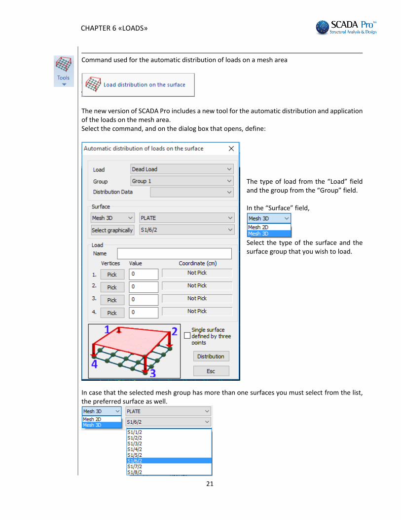
Command used for the automatic distribution of loads on a mesh area
The new version of SCADA Pro includes a new tool for the automatic distribution and application of the loads on the mesh area. Select the command, and on the dialog box that opens, define:
The type of load from the “Load” field and the group from the “Group” field. In the “Surface” field,
Select the type of the surface and the surface group that you wish to load.
In case that the selected mesh group has more than one surfaces you must select from the list, the preferred surface as well.
CHAPTER 6 «LOADS»
22
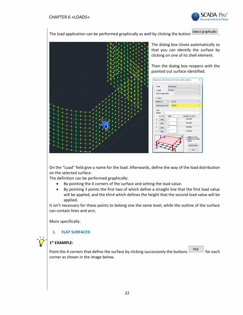
The load application can be performed graphically as well by clicking the button .
The dialog box closes automatically so that you can identify the surface by clicking on one of its shell element. Then the dialog box reopens with the pointed out surface identified.
On the “Load” field give a name for the load. Afterwards, define the way of the load distribution on the selected surface. The definition can be performed graphically:
By pointing the 4 corners of the surface and setting the load value.
By pointing 3 points the first two of which define a straight line that the first load value will be applied, and the third which defines the height that the second load value will be applied.
It isn’t necessary for these points to belong one the same level, while the outline of the surface can contain lines and arcs. More specifically:
1. FLAT SURFACES: 1st EXAMPLE:
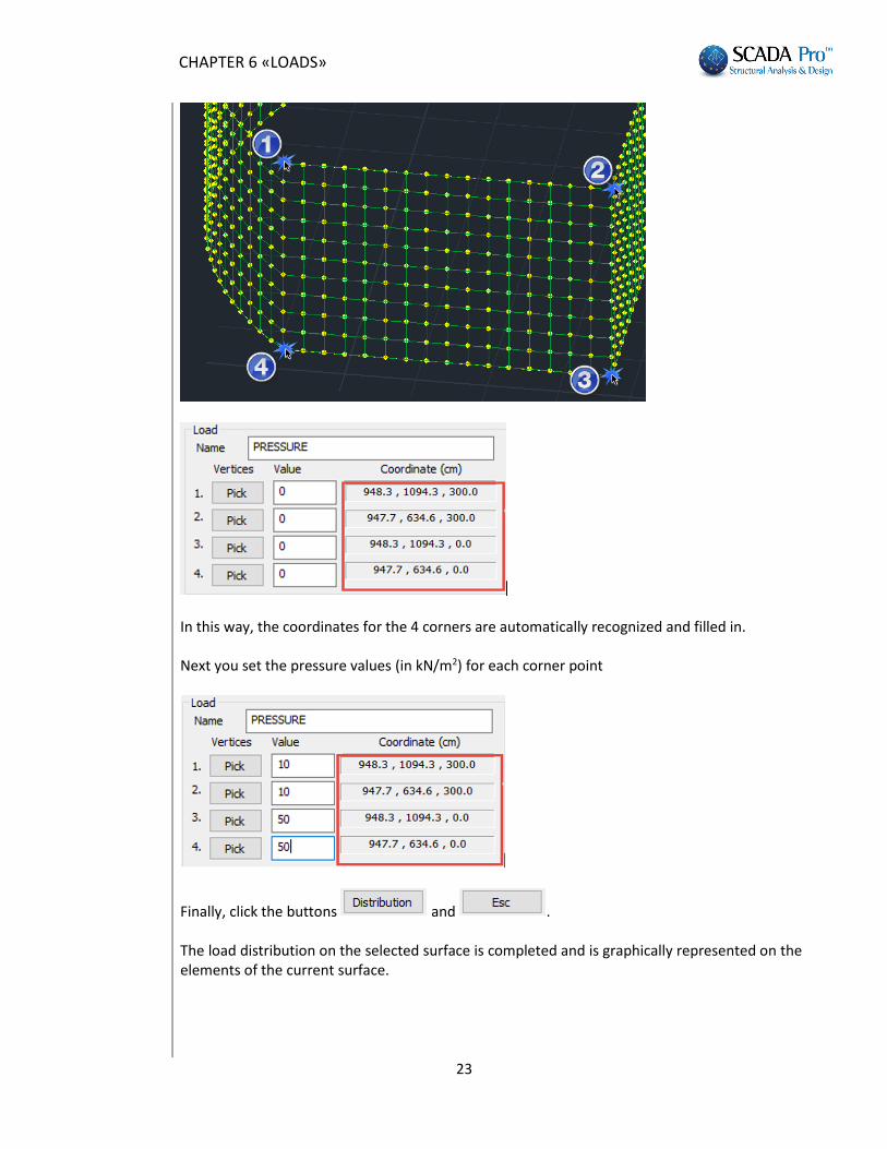
Point the 4 corners that define the surface by clicking successively the buttons for each corner as shown in the image below.
CHAPTER 6 «LOADS»
23
In this way, the coordinates for the 4 corners are automatically recognized and filled in. Next you set the pressure values (in kN/m2) for each corner point
Finally, click the buttons and . The load distribution on the selected surface is completed and is graphically represented on the elements of the current surface.
CHAPTER 6 «LOADS»
24
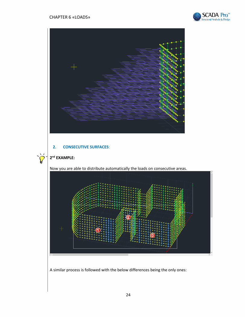
2. CONSECUTIVE SURFACES:
2nd EXAMPLE: Now you are able to distribute automatically the loads on consecutive areas.
A similar process is followed with the below differences being the only ones:

CHAPTER 6 «LOADS»
25
Using the “Select graphically” command you only select one element form one of the surfaces that are to be loaded.
Check the command “Single surface defined by three points” and the 4th option is automatically disabled.
As previously described, using the button, you point to the 3 points that define the combined area. Then specify the pressure values in kN / m2 for 3 points.
Finally, click the buttons and .

CHAPTER 6 «LOADS»
26
The load distribution on the selected surface is completed and is graphically represented on the elements of the current combined surface.
In order to distribute the loads to the rest of the surfaces, select again the command
and at the dialog box, click and select an element from the next surface that
is automatically recognized and selected from the list . Click
the buttons and .
Follow the same procedure for the third surface.

CHAPTER 6 «LOADS»
27
3. CURVED SURFACES: 3rd EXAMPLE:
Follow the same procedure:
Graphical selection with one click.
Check the option “Single surface defined by three points” and the 4th option is automatically disabled. Define the surface by pointing to the three points that define the
surface using the buttons. Fill in the pressure
values (in kN/m2) and click and .

CHAPTER 6 «LOADS»
28
1.4 Wind and Snow Loads
"Wind-Snow Loads" commands group contains tools for the automatic calculation of wind and snow loads, and the distribution to members in accordance with Eurocode 1.
Also Greek, Italian, Germany and Poland Eurocode 1 appendices and the Italian NTC08 Regulation are included. It is an extraordinary tool that includes:
Automatic calculation of characteristic values of snow load on the ground and on the roofs determined in accordance with EN 1990 for all types of roof: flat, single, double, quadruple, vaulted, with proximity roof tallest building drift in protrusions and obstacles of the Roof shape coefficients automatic calculation.
2D and 3D display of snow load distribution.
Basic wind velocity automatic calculation.
Automatic calculation of average wind speed VM (z) at height z (according to soil roughness and orography)
Categories and soil parameters
Wind turbulence
Max velocity
Wind pressure distribution on surfaces
Wind forces
Pressure coefficients for buildings (vertical walls or roofs) The procedure for calculating wind and snow loads and their distribution to members, includes 5 groups of commands:
1. Parameters: Code selection, Wind-snow general parameters 2. Edit: wall-roof 3. View: wind-snow 4. Member correspondence 5. Post-Processor

CHAPTER 6 «LOADS»
29
Parameters :
Code : In the dialog box that appears
Select the code for wind and snow loads calculation.
Wind : Define wind parameters in accordance with Eurocode 1 in the dialog box:
Select from the list: “Regulation” and “Zone” and the respect fields are automatically updated. In “Soil Type”: select type from the list, category and distance from the coast. In “Orthography Factor”: define topography and wind direction. The other fields are updated automatically based on the previous selections.

CHAPTER 6 «LOADS»
30
In “Roughness Factor”: when is activated, the program automatically
calculates the Cr(z) value, otherwise type a value manually. Press “OK” to save the parameters.
The user can modify the calculated values. By typing different values in the fields, data is updated automatically.
The latest version of SCADA Pro integrates the Saudi Arabia code (SBC 301) for wind loads as well. In the following a detailed description of the parameters choosing SBC 301 is described:
Wind : Selecting “Wind” parameters the following dialog box appears:
SBC 301 provides three methods for calculating wind loads (par. 6.1.2)

CHAPTER 6 «LOADS»
31
1. Simplified Procedure (Section 7.1) 2. Analytical Procedure (Section 7.2) 3. Wind Tunnel Procedure (Section 7.3) SCADA Pro incorporates the first two methods (The third method is based on experimental measurements).
First choose one of the two methods for the calculation of the wind loads . The first method applies only to buildings that meet specific criteria (par. 7.1.1).
The second parameter regards the choice of the class of the building
based on the Table 1.6-1. Press next to the parameter to open the corresponding table.
Then define the Base Wind Speed parameter based on the values of the
map (FIGURE 6.4-1) that appears when pressing .
The parameter regards the choice of the class exposure of the building in accordance with the paragraph 6.4.2.2 & 6.4.2.3.
Structural Type selection (TABLE 6.4-1) regards the choice of the Kd (Directionality Factor).
CHAPTER 6 «LOADS»
32
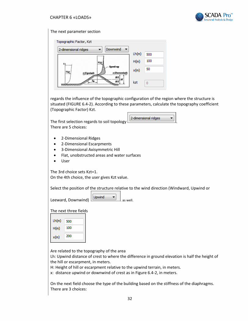
The next parameter section
regards the influence of the topographic configuration of the region where the structure is situated (FIGURE 6.4-2). According to these parameters, calculate the topography coefficient (Topographic Factor) Kzt.
The first selection regards to soil topology . There are 5 choices:
2-Dimensional Ridges
2-Dimensional Escarpments
3-Dimensional Axisymmetric Hill
Flat, unobstructed areas and water surfaces
User
The 3rd choice sets Kzt=1. On the 4th choice, the user gives Kzt value.
Select the position of the structure relative to the wind direction (Windward, Upwind or
Leeward, Downwind) . as well.
The next three fields
Are related to the topography of the area Lh: Upwind distance of crest to where the difference in ground elevation is half the height of the hill or escarpment, in meters. H: Height of hill or escarpment relative to the upwind terrain, in meters. x: distance upwind or downwind of crest as in Figure 6.4-2, in meters. On the next field choose the type of the building based on the stiffness of the diaphragms. There are 3 choices:
CHAPTER 6 «LOADS»
33
Rigid
Flexible
Parapets If defined as Flexible you must also set the following two parameters:
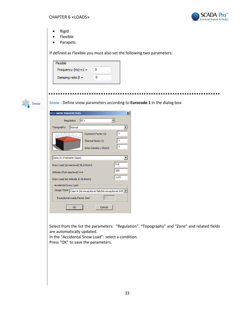
Snow : Define snow parameters according to Eurocode 1 in the dialog box:
Select from the list the parameters: “Regulation”. “Topography” and “Zone” and related fields are automatically updated. In the “Accidental Snow Load”: select a condition. Press “OK” to save the parameters.
CHAPTER 6 «LOADS»
34
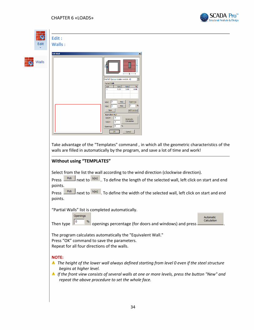
Edit : Walls :
Τake advantage of the "Templates" command , in which all the geometric characteristics of the
walls are filled in automatically by the program, and save a lot of time and work!
Without using “TEMPLATES” Select from the list the wall according to the wind direction (clockwise direction).
Press next to .. To define the length of the selected wall, left click on start and end points.
Press next to . To define the width of the selected wall, left click on start and end points. “Partial Walls” list is completed automatically.
Then type openings percentage (for doors and windows) and press . The program calculates automatically the "Equivalent Wall." Press “OK” command to save the parameters. Repeat for all four directions of the walls. NOTE:
The height of the lower wall always defined starting from level 0 even if the steel structure begins at higher level.
If the front view consists of several walls at one or more levels, press the button "New" and repeat the above procedure to set the whole face.

CHAPTER 6 «LOADS»
35
In this fill the table with the geometrical characteristics of the "Sub-walls".
Finally type the percentage of openings for each direction and press, every time,
the button . The program calculates automatically the “Equivalent Wall”.
All the front view should be circumscribed by the red rectangle.
“OK” to save the parameters. Repeat for all four directions of the walls.

CHAPTER 6 «LOADS»
36
Using “TEMPLATES”
Using "TEMPLATES" tool, the user saves a lot of time and work because the geometric characteristics of the walls are updated automatically by the program. Select from the list the wall according to the wind direction. “Partial Walls” list is completed automatically, without using “Pick” as previous.
The user needs only to type in the openings percentage and press . The program calculates automatically the "Equivalent Wall." Press “OK” to save the parameters. Repeat for all four directions of the walls.
Roofs :
Without using “TEMPLATES”
Select from the lists the roof number and the form.
Press next to “Peaks-Sides”. To define the geometry of the roof, left click on the four peaks of the floor plan of the roof and the cells will be filled in automatically.
Select from the lists and type in the height of the barrier in m. In “Geometrical Data” type in the number of frames and the other geometrical data in m. Roof Proximity
CHAPTER 6 «LOADS»
37
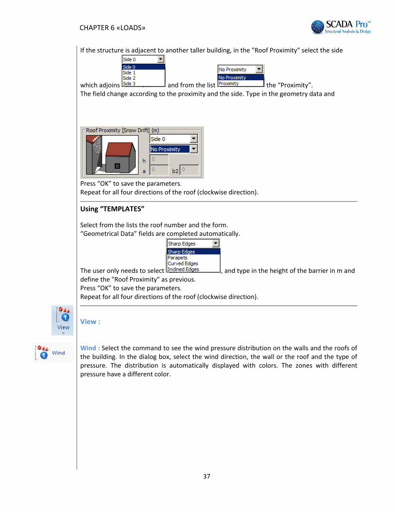
If the structure is adjacent to another taller building, in the "Roof Proximity" select the side
which adjoins and from the list the “Proximity”. The field change according to the proximity and the side. Type in the geometry data and
Press “OK” to save the parameters.
Repeat for all four directions of the roof (clockwise direction).
Using “TEMPLATES”
Select from the lists the roof number and the form. “Geometrical Data” fields are completed automatically.
The user only needs to select , and type in the height of the barrier in m and define the "Roof Proximity" as previous. Press “OK” to save the parameters.
Repeat for all four directions of the roof (clockwise direction).
View : Wind : Select the command to see the wind pressure distribution on the walls and the roofs of the building. In the dialog box, select the wind direction, the wall or the roof and the type of pressure. The distribution is automatically displayed with colors. The zones with different pressure have a different color.

CHAPTER 6 «LOADS»
38
Snow : Select the command to see the snow distribution on the roofs
In the dialog box, select from the list the number of "roof" of the "opening" i.e. the number of the frame, (if there are more than one), and "Case"
for the load distribution of snow.
Activate “Load” checkbox to display the values and “3DView” checkbox to receive snow distribution as is displayed in the following pictures.
CHAPTER 6 «LOADS»
39
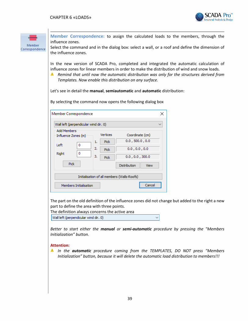
Member Correspondence: to assign the calculated loads to the members, through the influence zones. Select the command and in the dialog box: select a wall, or a roof and define the dimension of the influence zones. In the new version of SCADA Pro, completed and integrated the automatic calculation of influence zones for linear members in order to make the distribution of wind and snow loads.
Remind that until now the automatic distribution was only for the structures derived from Templates. Now enable this distribution on any surface.
Let's see in detail the manual, semiautomatic and automatic distribution: By selecting the command now opens the following dialog box
The part on the old definition of the influence zones did not change but added to the right a new part to define the area with three points. The definition always concerns the active area
Better to start either the manual or semi-automatic procedure by pressing the "Members Initialization” button. Attention:
In the automatic procedure coming from the TEMPLATES, DO NOT press "Members Initialization” button, because it will delete the automatic load distribution to members!!!

CHAPTER 6 «LOADS»
40
Manual Procedure - Without using “TEMPLATES”
In define the influence zones of a member by typing the corresponding widths in m, left and right of that, "Pick" and left click on the member (or parts of the member). The “Influence Zone” is displayed as in the figure below.
“Left” and “Right” determined based on the local axis x (red).
Semi-automatic Procedure - Without using “TEMPLATES”
Added to the right a new part to define the area with three points. The definition always concerns the active area:
Better to start the procedure by pressing the "Members Initialization” button. Indicate the point graphically with the following particularity: The first two points define the direction by which the automatic calculation of influence
surfaces made for items which are parallel to this direction.
CHAPTER 6 «LOADS»
41
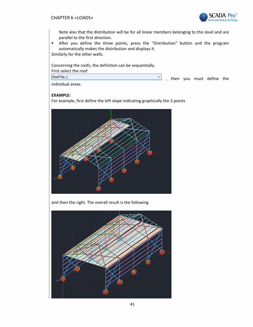
Note also that the distribution will be for all linear members belonging to this level and are parallel to the first direction.
After you define the three points, press the "Distribution" button and the program automatically makes the distribution and displays it.
Similarly for the other walls. Concerning the roofs, the definition can be sequentially. First select the roof
, then you must define the individual areas. EXAMPLE: For example, first define the left slope indicating graphically the 3 points
and then the right. The overall result is the following

CHAPTER 6 «LOADS»
42
Finally it is worth noting that if the walls are properly defined there is NO need of more
definition. Just select each wall and press «Distribution». The distribution becomes and simultaneously displays on the linear members belonging to this wall.
Same for the flat roofs only.
Automatic Procedure - Using “TEMPLATES”
Activated “Purlins” and “Girders” in “Load Attribution” of “Templates”
, just select "Pick" and the program automatically calculates the influence zones distributing the pressure in all purlins and girders.
CHAPTER 6 «LOADS»
43
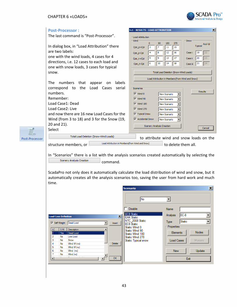
Post-Processor :
The last command is “Post-Processor”. In dialog box, in “Load Attribution” there are two labels:
4. one with the wind loads, 4 cases for 4 directions, i.e. 12 cases to each load and
5. one with snow loads, 3 cases for typical snow. The numbers that appear on labels correspond to the Load Cases serial numbers.
Remember: 6. Load Case1: Dead 7. Load Case2: Live
and now there are 16 new Load Cases for the Wind (from 3 to 18) and 3 for the Snow (19, 20 and 21). Select
to attribute wind and snow loads on the
structure members, or to delete them all. In “Scenarios” there is a list with the analysis scenarios created automatically by selecting the
command.
ScadaPro not only does it automatically calculate the load distribution of wind and snow, but it automatically creates all the analysis scenarios too, saving the user from hard work and much time.

CHAPTER 6 «LOADS»
44
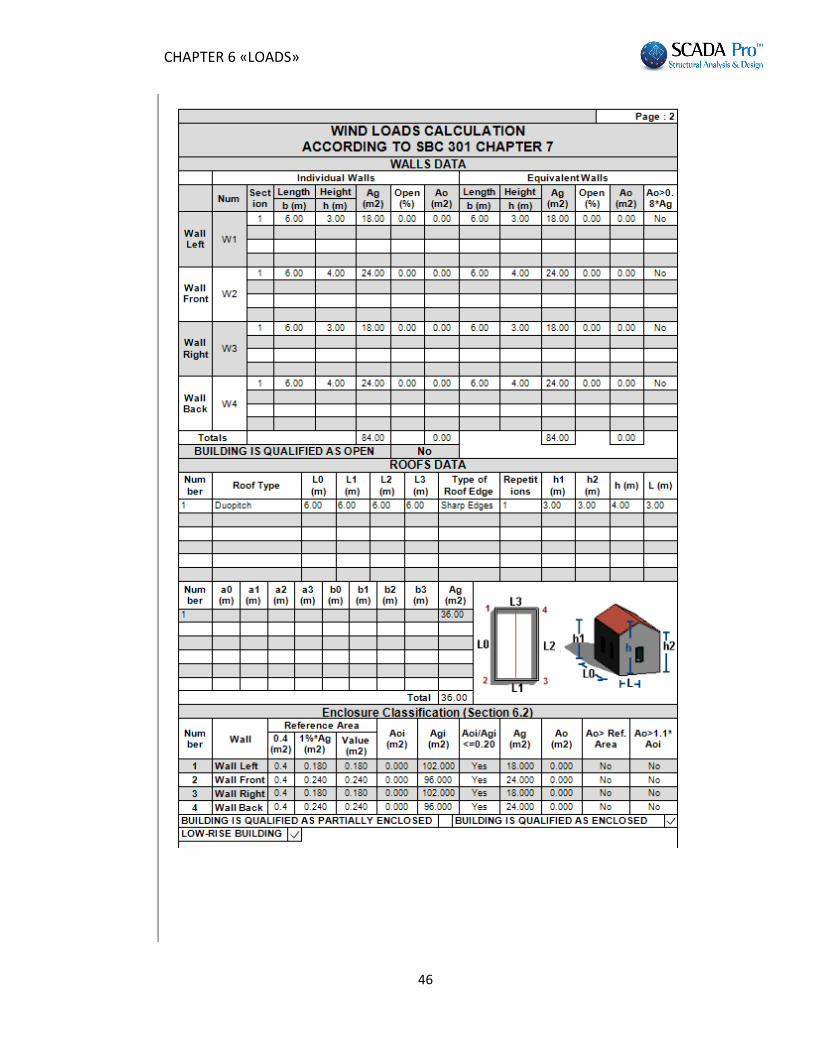
Press to open the txt results file, containing in detail all data and calculations derived from all Eurocode 1 procedure.
Choosing the SBC 301 Regulation, the printing is as follows:

CHAPTER 6 «LOADS»
45
CHAPTER 6 «LOADS»
46