chapter 6: isotopes

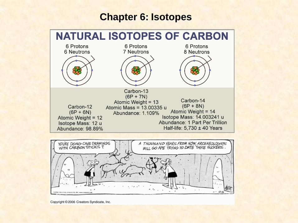
Chapter 6: Isotopes

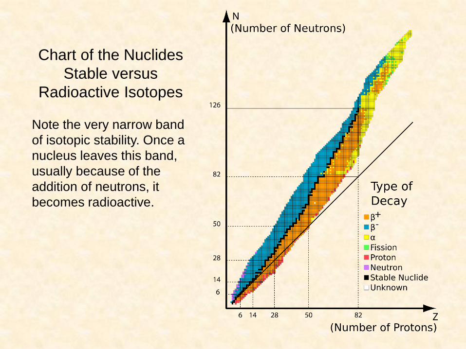
Chart of the Nuclides

Stable versus

Radioactive Isotopes

Note the very narrow band

of isotopic stability. Once a

nucleus leaves this band,

usually because of the

addition of neutrons, it

becomes radioactive.

Types of Radioactive Decay

Radioactive Decay and Growth

The decay of a radioactive isotope is a first-order reaction and can be

written:

dN/dt =-N

Where N is the number of unchanged atoms at the time t and is

the radioactive decay constant.

This equation can be rewritten as:

N = Noe-t

Where No is the number of atoms present at t = 0. This is the basic

form of the radioactive decay equation.

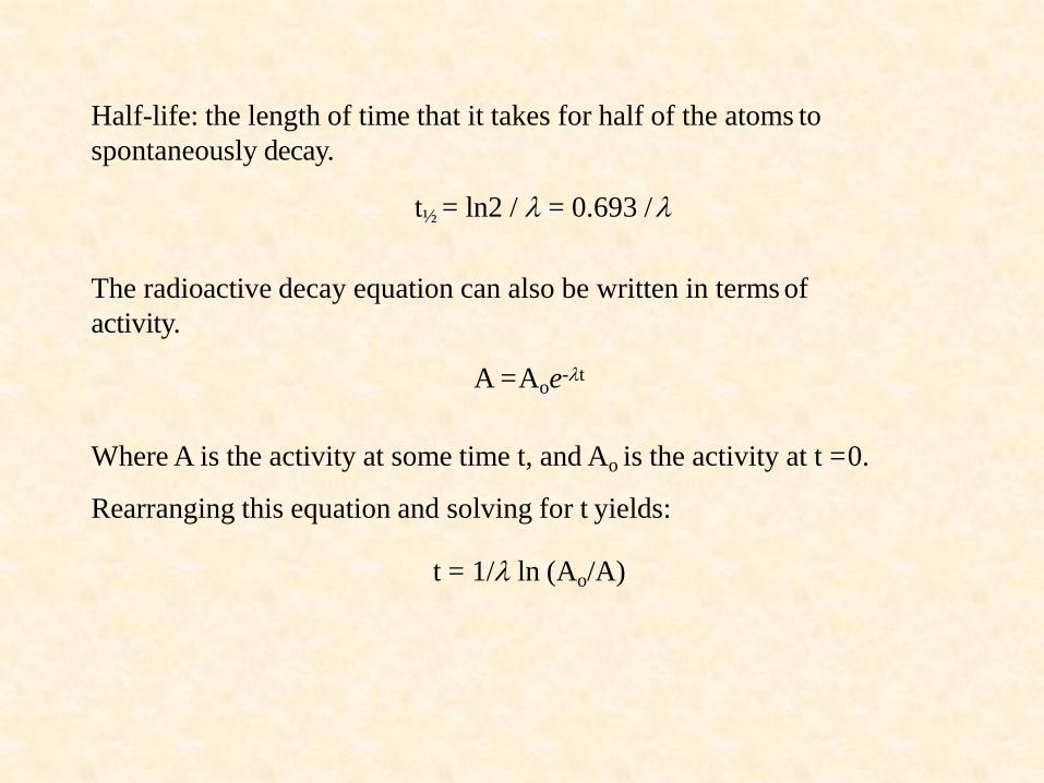
Half-life: the length of time that it takes for half of the atoms to

spontaneously decay.

t½ = ln2 / = 0.693 /

The radioactive decay equation can also be written in terms of

activity.

A = Aoe-t

Where A is the activity at some time t, and Ao is the activity at t = 0.

Rearranging this equation and solving for t yields:

t = 1/ ln (Ao/A)

In practice, it is often easier to consider radioactive decay in

terms of a radioactive parent and radioactive progeny (daughter).

**For any closed system, the number of progeny atoms plus the

number of parent atoms remaining must equal the total number

of parent atoms at the start. Solving for time yields the

following equation:

t = 1/ ln[1 + (P/N)]

Where N = the number of parent atoms and P = the number of

progeny atoms produced.

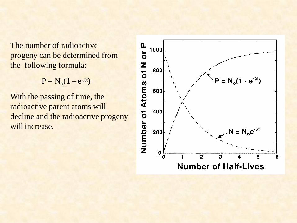
The number of radioactive

progeny can be determined from

the following formula:

P = No(1 – e-t)

With the passing of time, the

radioactive parent atoms will

decline and the radioactive progeny

will increase.

Measurement of Radioactivity

Becquerel (Bq) is the basic measurement of radioactivity. 1Bq =

1.000 disintegrations per second.

Curie (Ci) another commonly used measurement of radioactivity. 1Ci

= 3.700 x 1010 disintegrations per second. A picocurie is 1 x 10-12

curies.

Gray (Gy): the unit used in the study of the chemical and biological

effects of radiation. A dose of 1Gy deposits 1 joule of energy per

kilogram of material.

Rad: another often-used unit where 1Gy = 100 rad.

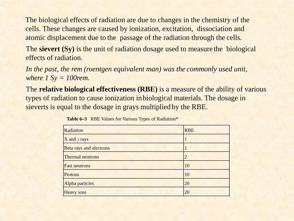
The biological effects of radiation are due to changes in the chemistry of the

cells. These changes are caused by ionization, excitation, dissociation and

atomic displacement due to the passage of the radiation through the cells.

The sievert (Sy) is the unit of radiation dosage used to measure the biological

effects of radiation.

In the past, the rem (roentgen equivalent man) was the commonly used unit,

where 1 Sy = 100rem.

The relative biological effectiveness (RBE) is a measure of the ability of various

types of radiation to cause ionization in biological materials. The dosage in

sieverts is equal to the dosage in grays multiplied by the RBE.

Radiation RBE

X and γ rays 1

Beta rays and electrons 1

Thermal neutrons 2

Fast neutrons 10

Protons 10

Alpha particles 20

Heavy ions 20

Table 6–3 RBE Values for Various Types of Radiation*

Tritium dating

There are three isotopes of hydrogen: 1H, 2H (deuterium), and 3H

(tritium), with average terrestrial abundances (in atomic %) of

99.985, 0.015 and <10-14 respectively.

Tritium is radioactive and has a half-life of t½ = 12.43 years. This means it is

used to date sample that are less than 50 years old.

Tritium is produced in the upper atmosphere by the bombardment of nitrogen

with cosmic-ray produced neutrons.

𝑁 + 𝑛 → 3 𝐻𝑒24

714 + 𝐻1

3

The production rate is 0.5 ± 0.3 atoms cm-2 sec-1

Tritium abundances are measured in several ways:

tritium unit (TU) = 1 tritium atom per 1018 hydrogen atoms

dpm L-1 = disintegrations per minute per liter

pCi L-1 picocuries per liter (of water.)

1TU = 7.1 dpm L-1 = 3.25 pCi L-1

From the onset of of atmospheric testing of fusion bombs in 1952, until

the signing of the Atmospheric Test Ban Treaty in 1963, bomb- produced

tritium was the major source of tritium. Prior to the testing of fusion

devices, the tritium content of precipitation was probably between 2 and

8TU. A peak of several thousand TU was recorded in the northern

hemisphere precipitation in 1963.

Event dating describes the

marking of a specific period

where the abundances of an

isotope are uncharacteristically

elevated or diminished. For

example, groundwaters that

were recharged between 1952

and 1963 will have a distinctive

signature indicating an increase

in 3H production.

Tritium decays through - emission. This means that the parent material

is 3H and the progeny material is 3He.

Given T = 5.575 x 10-2 y-1, if through sampling ground water you find 3H

= 25TU and 3He = 0.8TU, what time has passed since that groundwater

was recharged (at the surface)?

Recall: t = 1/·ln[1 + (P/N)]

t = 17.937·ln[1 + (0.8/25)] = 0.6 y

Carbon – 14 Dating

14C has been used for dating samples

that are roughly 50,000 years old or

younger (accelerator mass

spectrometry ups the usage to 100,000

years). There are 3 isotopes of carbon: 12C, 13C, & 14C, with average terrestrial

abundances of 98.90, 1.10, and <10-10,

respectively. 14C is the only radioactive

carbon isotope with a half-life of 5,730

years.

𝑁 + 𝑛 → 𝐻11

714 + 𝐶6

14

𝐶 → 𝑁714

614 + β- + 𝜈 + Q

t = 1

1.209 𝑥 10_4 ln(

𝐴𝑜

𝐴)

In order to use 14C for geochronology, it is assumed that the atmosphere is

in secular equilibrium with respect to 14C. Meaning that the rate at which 14C is produced by cosmic ray flux is equal to the rate of decay of 14C, so

the abundance of 14C in the atmosphere remains constant. However, for a

variety of reasons, the abundance of 14C has not remained constant over

time. These variations need to be accounted for when using this dating

method.

In order to calibrate the C-14 time

scale one must use carbon-

containing materials of known age.

A popular choice is the bristlecone

pine, the oldest of which has an

age of almost 5,000 years.

U-Series Disequilibrium Methods of Dating

For a system that has been closed for a sufficiently long time, secular

equilibrium will be achieved and the relative abundance of each isotope

will be constant.

When the system enters disequilibrium due to separation of either

parent or progeny, or subsequent decay, the reestablishment of

equilibrium can be used as a dating method.

For example, when 234U decays to 230Th in sea water, the 230Th is rapidly

removed from sea water because, unlike uranium, thorium is very

insoluble (reactive). In this case, the 230Th that accumulates in the

sediments is said to be unsupported, as it is now separated from its

parent isotope.

Table 6-1. Uranium decay series*

Uranium 238 Uranium 235

Isotope

Emitted

particle Half-life Isotope

Emitted

particle Half-life

238

92U α 4.47 x 109 yrs235

92U α 7.038 x 108 yrs

234

90Th β - 24.1 days231

90Th β- 1.063 days

234

91Pa β - 1.17 min231

91Pa α 3.248 x 104 yrs

234

92U α 2.48 x 105 yrs227

89Ac β- 21.77 yrs

230

90Th α 7.52 x 104 yrs227

90Th α 18.72 days

226

88Ra α 1.60 x 103 yrs223

88Ra α 11.435 days

222

86Rn α 3.8235 days219

86Rn α 3.96 sec

218

84Po α 3.10 min215

84Po α 1.78 x 10-3 sec

214

82Pb β - 27 min211

82Pb β- 36.1 min

214

83Bi β - 19.9 min211

83Bi α 2.14 min

214

84Po α 1.64 x 10-4 sec207

81Tl β- 4.77 min

210

82Pb β - 22.3 yrs207

82Pb Stable

210

83Bi β - 5.01 days

210

84Po α 138.38 days

206

82Pb Stable

*Data source: Chart of the Nuclides (1989).

Isotope Isotope

238

92U235

92U

234

90Th231

90Th

234

91Pa231

91Pa

234

92U227

89Ac

230

90Th227

90Th

226

88Ra223

88Ra

222

86Rn219

86Rn

218

84Po215

84Po

214

82Pb211

82Pb

214

83Bi211

83Bi

214

84Po207

81Tl

210

82Pb207

82Pb

210

83Bi

210

84Po

206

82Pb


Table 6-2. Thorium decay series*

Isotope

Emitted

particle Half-life Isotope

Emitted

particle Half-life

232

90Th α 1.40 x 1010 yrs216

84Po α 0.145 sec

228

88Ra β - 5.76 yrs212

82Pb β- 10.64 hr

228

89Ac β - 6.15 hr

212

83Bi α (33.7%)

β - (66.3%)

1.009 hr

228

90Th α 1.913 yrs 208

81Tl β- 3.053 min

224

88Ra α 3.66 days 212

84Po α 2.98 x 10-7 sec

220

86Rn α 55.6 sec208

82Pb Stable


212

83Bi

208

81Tl

212

84Po

208

82Pb

230Th Dating of Marine Sediments:

As we saw in the last example, 230Th is reactive in the marine

environment (i.e., it is rapidly removed from seawater by particles).

In fact it has a mean residence time of about 300 years.

Given that the addition and removal of U (230Th’s parent) to the

ocean is in balance (U has a residence time in seawater of about 1

million years), 230Th is produced at a constant rate. This means

that as long as there has been no disruption to the sediment layers

on the sea floor, the uppermost layer will represent present-day 230Th deposition to the sediments.

230Th = 9.217 x 10-6 y-1.

t = 108,495 ln(230Thinitial / 230Thmeasured)

Example 6-4

The 230Th activity is measured for a marine sediment core. The top

layer of the core has a 230Th activity of 62 dpm. At a depth of 1m, the 230Th activity is 28 dpm. Calculate the age of the sediment at a depth of

1m.

t = 108,495 ln(62/28) = 86,246 y

Rate = (sediment thickness / time) = 1m / 86,246 y = 1.16 cm /1000 y.

230Th / 232Th Sediment Dating

This method uses the ratio of these two radioisotopes instead of

just 230Th. In this case the age equation is

t = 1/ln (R0 / R) = 108,495 ln (R0 / R)

Where……

R = 230Th / 232Th measured

R0 = 230Th / 232Th initial

R is also = (230Th / 232Th)0 e-t

So far the examples have been for ‘unsupported’ activity. We have

assumed that parent and progeny are separated.

Supported activity – case where a parent or grandparent was originally

present in the sediment. Decay of this parent and/or grandparent contributes

to the total activity of the progeny.

238U 234U 230Th

230Th

230Th = Thorium scavenged from the water column = unsupported acitvity

230Th = Thorium produced from 238U in the particle = supported activity

Total activity = 230Th 230Th +

particle

230Th / 231Pa Sediment Dating

Very similar to the 230Th / 232Th except the half life is shorter, so you

can use it for somewhat faster accumulation rates.

Activity and Sediment-Rate Relationships

Radioactive decay is a first-order process (i.e. exponential decay)

If sedimentation is constant then the sedimentation rate (a) = ( /-2.303m)

m is the slope

Stochastic system has a random probability distribution or pattern that may

be analyzed statistically but may not be predicted precisely.

Deterministic system is a system in which no randomness is involved in the

development of future states of the system. Can accurately predict future

states.

238

206 206 238

204 204 204

meas initial

Pb Pb U( 1)

Pb Pb Pb

te

235

207 207 235

204 204 204

meas initial

Pb Pb U( 1)

Pb Pb Pb

te

232

208 208 232

204 204 204

meas initial

Pb Pb U( 1)

Pb Pb Pb

te

U-Th-Pb isotopic systems

Stable Isotopes

Do not spontaneously breakdown to form other isotopes

Table 6-6. Average terrestrial abun dances of stable isotopes

used in en viron mental stu dies*

Element

Average Terrestrial

Abundance (atom %)

Hydrogen

Carbon

Nitrogen

O xygen

Sulfur

99.985

0.015

98.9

1.1

99.63

0.37

99.762

0.038

0.2

95.02

0.75

4.21

0.014

Isotope

1

1H

1

2H

6

12C

6

13C

7

14N

7

15N

8

16O

8

17O

8

18O

16

32S

16

33S

34S

16

16subp36 S

*Data source: IUPAC (1992).

Isotopic Fractionation – partitioning of isotopes during phase change

or reactions. Partitioning is proportional to the masses of the isotopes.

Equilibrium Fractionation: forward and backward reaction rates are

equal for each isotope.

Bi-directional reactions at equilibrium (like water vapor over water)

Lighter isotopes in the gas phase (lighter isotopes = more kinetic

energy).

Example: evaporation of water in a closed space

Kinetic Fractionation: unidirectional reactions in which reaction rates

are dependent on the masses of the isotopes and their vibrational

energies.

Example: breakdown of calcite in an acid solution to produce Ca2+ and

CO2 (g) . The gas escapes and therefore doesn’t equilibrate with the

calcite.

Fractionation Factor

Describes the partitioning of stable isotopes between two substances, A and B

= RA / RB

where R is the ratio of the heavy to light isotope of the element for each

substance and α is the fractionation factor

The fractionation factor

varies as a function of

temperature and at high

temperature it

approaches unity.

The (delta notation)

= [(Rsamp – Rstd) / Rstd] x 1000

same as

= [(Rsamp / Rstd) -1] x 1000

R is the ratio of the heavy to light isotope. Various standards are used

depending on the element.

Units are per mil “‰”

Table 6–7 Stable Isotope Ratios for Standards (Data from Kyser (1987)).

Element Standard Ratio

Hydrogen V-SMOW 2H/1H = 155.76 × 10−6

Carbon PDB 13C/12C = 1123.75 × 10−5

Oxygen V-SMOW 18O/16O = 2005.2 × 10−6

PDB 18O/16O = 2067.2 × 10−6

Nitrogen NBS-14 15N/14N = 367.6 × 10−5

Sulfur CDT 34S/32S = 449.94 × 10−4

EXAMPLE 6–5 The isotopic ratio of 18

O/16

O in V-SMOW is 0.0020052. A rainwater sample

collected in Boston, Massachusetts, has an 18

O/16

O ratio of 0.0019750. Calculate the delta value

for this rainwater sample.

sample standard

standard

Ratio Ratio 0.0019750 0.00200521000 1000

Ratio 0.0020052

15.1‰

The delta value is reported in parts-per-thousand (‰), and the negative value means that the

sample is isotopically lighter than the standard.

Rearranging the delta-notation equation and combining it with the

fractionation factor () equation allows for calculation of the delta value of

one compartment if you know the delta value for the other compartment.

= RA/RB = (A + 1000) / (B + 1000)

Oxygen and Hydrogen Isotopes in Water

Used for ‘sourcing’ water

For hydrogen we use 1H and 2H (deuterium, D)

For oxygen we use 16O and 18O

values for O and H in water are zero for seawater.

For water vapor in equilibrium with seawater at 25ºC - D = -69 ‰

and 180 = -9.1 ‰

For water vapor in equilibrium with seawater at 10ºC - D = -84 ‰

and 180 = -10.1 ‰

Temperature effects the fractionation from liquid to vapor phase

for H and O. The temperature effect comes into play both for

latitude and altitude. This temperature effect on fractionation is

what gives rise to different isotopic values In H and O for different

areas of precipitation.

The process of fractionation during condensation

Start with water vapor that is isotopically light in H and O relative to

seawater

As the vapor begins to condense out into clouds

Initial droplets are rich in 18O and D

Vapor becomes more depleted in 18O and D

As condensation continues-

Vapor becomes more depleted

Droplets in turn reflect lower 18O

and D coming from source vapor

The change in isotopic value of both

the vapor and liquid is a function of

how much of the original vapor is

left.

Described by a Rayleigh Distillation function

Rayleigh Distillation (or fractionation)

18Ov = [18O0 + 1000] f (-1)

vapor

fraction

remaining

starting

vapor

To relate the condensing liquid to the vapor

18Ol = (18Ov + 1000) - 1000

This process results in:

-rain early in a precip event is isotopically heavier than at the

end of the event

-delta values of rain decreases from coastal to inland areas

-rain is isotopically lighter at the poles

The H and O isotopes in precipitation are related:

D = 8 18O + 10 (excess of D relative to 18O; d)

or

D = 8 18O + d , where d is the D excess

Isotope fractionation of H and O in water (during condensation)

Figure 6-6. Plot of D versus 18O illustrating the mean global meteoric water line and

local meteoric water lines. Other processes that affect the isotopic ratios - e.g., low-

temperature water-rock exchange, geothermal exchange, and evaporation - are also

illustrated. A and B are two water masses and the dashed line represents the possible

isotopic compositions of water produced by mixing of these two end members. The

diagram is modified from “Uses of Environmental Isotopes” by T. B. Coplen in

REGIONAL GROUND WATER QUALITY edited by W. M. Alley, pp. 227-254.

Copyright © 1993. This material is used by permission of John Wiley & Sons, Inc.

D = 8 18O + 10

Is the equation for the

Global Meteoric Water Line

This has nothing to do with

meteors

Different areas influenced by evaporation, water-rock

interaction, etc. will cause a deviation in the D excess ()

relative to 18O in water.

It is the different D values relative to the GMWL that allows

you to ‘tag’ water masses.

With this tag you can examine contributions of different water sources

to ground and surface waters.

Example 6-7: River flow below a dam is a mixture of water coming from the

reservoir behind the dam and from a groundwater source.

River…..18O = -3.6‰ , D = -44.6 ‰

Res….. 18O = -4.5‰ , D = -38 ‰

GW…. 18O = -3.0‰ , D = -49 ‰

What's the percentage contribution of each source?

This is a two-endmember mixing problem.

For D…….fGW DGW + fres Dres = Driv

+ fres 18Ores = 18Oriv

2 equations, 2 unknowns,

Redefine fGW in terms of fres,

Substitute and solve sequentially

f1 = 0.40

f2 = 0.60

GW supplies 40% of the water in the river

Reservoir supplies 60% of the water in the river

For 18O… fGW 18OGW

Also fGW + fRES = 1

Climate Change

Because the fractionation of H and O in water changes with temp, isotopic

measurements of ice-cores are used to estimate paleoclimate.

1) Isotopic composition of snow reflects air temp.

2) Colder air = more negative D and 18O

3) Warmer air = less negative D and 18O

4) Works the same in both hemispheres

5) Once snow is packed into glacier, ice stratigraphy not disturbed,

paleothermometer locked into place

Ice ages can confound this approach to some extent because by locking up

a bunch of ocean water into glaciers, the overall D and 18O of all water

gets less negative. This effect is small relative to the temp effect.

Arctic Antarctic When records from both hemispheres agree, it is

a global climate change

When the disagree, it is a local climate change

Antarctic

Carbon

We can use 13C to detect

fossil fuel contributions to

atmospheric CO2. The

Suess effect.

-7‰

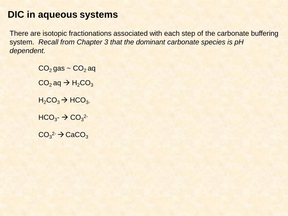
DIC in aqueous systems

There are isotopic fractionations associated with each step of the carbonate buffering

system. Recall from Chapter 3 that the dominant carbonate species is pH

dependent.

CO2 gas ~ CO2 aq

CO2 aq H2CO3

H2CO3 HCO3-

HCO3- CO32-

CO32- CaCO3

Figure 6-10. Isotopic fractionation factors, relative to CO2 gas, for

carbonate species as a function of temperature. Deines et al. (1974).

Table 6-8. Fractionation factors for

carbonate species relative to gaseous CO2 *

1000 ln α = -0.91 + 0.0063 106/T2

1000 ln α = -4.54 + 1.099 106/T2

1000 ln α = -3.4 + 0.87 106/T2

1000 ln α = -3.63 + 1.194 106/T2

*From Deines et al. (1974).

H2CO3

HCO3-

CO 2

3

Ca CO3 (s)

Isotopic composition of DIC also

depends on open vs closed

system.

Using Equations in Table 6-8

Example 6-8: CaCO3 is ppt in water in equilibrium with the atm. What is the 13C

for the carbonate at 25ºC.

CaCO3 relative to CO2g: 1000ln = -3.63 + 1.194 x 106/T2

= 9.8….calcite is 9.8‰ heavier than CO2g

CO2g = -7‰, so calcite is 2.8‰

g

Example 6-9: Bicarb in ocean dominate DIC. What is the 13C

for DIC in the ocean at 10ºC.

HCO3- relative to CO2g: 1000ln = -4.54 + 1.099 x 106/T2

= 9.18..bicarb is 9.18‰ heavier than CO2

Bicarb dominates DIC so …

CO2g = -7‰, therefore ocean 13 DIC = 2.8‰

Methane

Figure 6-11. 13C and deuterium isotopic values

for methane from various sources and reservoirs.

M

- abiogenic (from the mantle), P - petroleum, A -

atmosphere, G - geothermal (pyrolitic from

interaction with magmatic heat), T - thermogenic

(from kerogen at elevated temperatures), F -

acetate fermentation (bacterial), and R - CO2

reduction (bacterial). After Schoell (1984, 1988).

This technique, at least

the carbon part, has

been used to determine

whether some deep-sea

methane-based

communities are fueled

by thermogenic or

biogenic methane

deposits.

Methane hydrates, biogenic in origin

13C average of about -65 ‰ (range -40 to -

100‰)

Carbon isotopes – food webs, paleo or otherwise.

C3 plants (deciduous trees) – 13C = -15‰

C4 plants (grasses, marsh, corn…) – 13C = -30‰

plankton – 13C = -22‰

Small trophic fractionation …about 1 ‰

1

5N

carnivores

herbivores

13C

Nitrogen

Stable isotopes of N and O used to trace sources of nitrogen pollution

usually in the form of NO3- or NH3

15N can be substantially altered by biological processes

Nitrates in surface and groundwater

Fertilizer 15N = 0 ‰

Manure 15N = 15 ‰ ± 10‰

In theory you can use 15N to distinguish

sources. In practice, it’s difficult……

Nitrate is reactive in surface and groundwaters undergoing denitrificaiton.

As denitrification converts nitrate to N2, the residual nitrate becomes isotopically

heavier. So a fertilizer source of nitrate that has undergone some denitrification

will start to look isotopically like the manure nitrate.

A way to constrain this problem is to also measure 18O in nitrate

Fertilizer 18O = +23 ‰ (oxygen in nitrate comes from air)

Manure 18O = -10‰ (oxygen in nitrate comes mostly from water)

During denitrificaiton, both O and N are fractionated but their fractionations

relative to each other are predictable

Figure 6-12. Determination of the relative importance of

nitrate sources to a groundwater system. Two sources for

nitrates are fertilizer and manure. Both are undergoing

denitrification. A and B represent each source at a particular

stage in the denitrification process. C is the isotopic

composition of the nitrate in the groundwater due to simple

mixing. In this example, approximately 60% of the nitrate is

contributed by the fertilizer.

Red circles = measurements

Draw the predicted fractionation lines

for each end-member (blue lines).

Note they have the same slope

Draw a line through the measured

GW sample (the mixture) that is

perpendicular to the fractionation slopes

(dashed line)

Now you can either do a mixing calc

to determine fraction of each source, or

Amount of A = C-B / A-C

The ‘lever law’…just like torque in physics

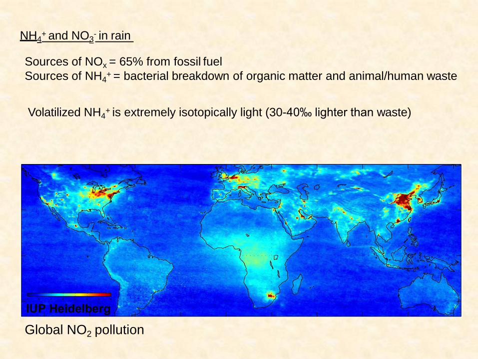
NH4+ and NO3

- in rain

Sources of NOx = 65% from fossil fuel

Sources of NH4+ = bacterial breakdown of organic matter and animal/human waste

Volatilized NH4

+ is extremely isotopically light (30-40‰ lighter than waste)

Global NO2 pollution

Sulfur

Big isotopic difference between

sulfides and sulfates

Sulfate reduction (microbial) has

a big fractionation, as does microbial

sulfide oxidation

Is the sulfide produced during sulfate

reduction isotopically lighter or heavier

than the sulfate?

What’s the major source of sulfate on

the planet?

Burning fossil fuels…

Mixing

Binary mixing

mix = AfA + B(1-fA)

If the two sources have unequal concentrations of the element of interest, the

mixing equation must be weighted to reflect that:

mix = AfA(A/M) + B(1-fA)(B/M)

…..where A,B, and M are the concentrations

of source A, B, and the mixture with respect to the element of interest.

Mixing with more than two end members

Figure 6-14. Plot of PO43- versus NO3

- in water

samples from feedlot runoff (M), cultivated fields (F),

uncontaminated groundwater (G), and contaminated

well water (W). The sample of contaminated well water

falls within the triangle defined by compositions M, G,

and F, indicating that this sample is a mixture of these

three compositions. The relative proportions of each

end member can be determined by applying the lever

rule (see Example 6-11).

Paleothermometry – using carbonates

18O in carbonate

Fractionation factor governing water (oxygen) equilibration with CaCO3

is

temperature dependent

t (ºC) = 16.9 – 4.14(18Ocalcite – 18Owater) + 0.13(18Ocalcite – 18Owater)2

Due to large and seasonal variations in freshwater oxygen isotopes,

only oceanic carbonate organisms work.

Lots of other assumptions and corrections so the tool is used as a

relative indicator of paleotemperature.

chapter 6: isotopes

Documents