1

McPeak Lecture 7

PAI 723 Firms and Production

Firms:

Three main kinds.

1) Sole proprietorships

2) Partnerships

3) Corporations (Limited Liability)

Objective of the firm: make decisions so as to maximize

profit.

Profit is defined as revenue, what it earns from selling the

good, minus costs, what it costs to produce the good.

CR or, in slightly different form

xw)x(fp

2

Necessary vs. sufficient conditions.

A necessary condition is in the nature of a prerequisite.

Statement A is true only if another statement B is true,

then “A only if B” or “If A, then B”.

If a person is a father, then they are a male.

If Felix is a cat, then Felix hates baths.

Felix is a cat only if he hates baths.

If A (cat), then B (hates baths).

Can we turn it around: If B (hates baths), then A (cat)?

If Felix hates baths, can we assume Felix is a cat?

No, Felix might be a four year old boy for example.

Felix hating baths is a necessary condition for Felix to be

a cat, but it is not sufficient. It is one characteristic of

being a cat, but this characteristic is shared by non-cats as

well.

3

Consider the situation where A is true if B is true, but A

can be true when B is not true. B is a sufficient condition

for A.

A is “one can get to Chicago from Syracuse”,

B is “One can take a plane to Chicago from Syracuse”,

then the truth of B suffices for the establishment of the

truth of A, but is not a necessary condition for A to be

true. B is a sufficient condition for A but not a necessary

one.

Consider where A and B imply each other.

A is “it is the month of February”. B is “there are less

than 30 days in the month”. A is a necessary and

sufficient condition for B, and vice versa.

4

Back to economics.

The point (x1, x2) being on the budget line is necessary

but not sufficient for the point (x1, x2) to be the optimal

bundle.

Yes it has to be on the budget line, but other

conditions need to be met as well. A lot of non-

optimal bundle points are on the budget line as well.

We need to get a condition that takes care of these.

The reverse statement is a sufficient condition: the

point (x1,x2) is the optimal bundle, therefore it lies

on the budget line.

The point (x1,x2) is the point where MRS=MRT implies

the point (x1,x2) the optimal bundle.

MRS=MRT implies optimal bundle, and optimal

bundle implies MRS=MRT.

5

Technologically efficient production is a necessary

condition for profit maximization.

Profit maximization is sufficient for technologically

efficient production.

Profit max implies we are technologically efficient, but

being technologically efficient is not enough to know we

are producing at a profit maximizing level.

Technologically efficient production: the firm can not

produce more output given the amount of inputs it is

using, and the firm cannot produce the amount of output it

is producing by using fewer inputs.

Show sets.

Production function.

A firm gathers together inputs, or factors of production.

The firm then applies a technology, or production process

to these inputs.

The result is an output – can be a good or a service.

No costs of input are involved yet.

6

No selling of the product is going on yet.

Just (boring old) production!!!!

7

Define a production function Q=f(K,L,E,M)

Q is output of the good (in many studies, people use Y

rather than Q – means the same thing)

K is capital

L is labor

E is energy

M is materials

f (.) defines the relationship between the quantities of

inputs used and the maximum quantity of output that can

be produced given current knowledge about technology

and organization.

What is the nature of the f(.)? It can take on lots of

different forms.

An important part of econometric work is to estimate the

nature of the production function.

8

We can treat inputs in the production function as fixed or

variable inputs.

In the short run, factors of production that can not easily

be varied are viewed as fixed inputs.

A factor for which it is relatively easy to adjust the

quantity quickly is a variable input.

The long run is the time span required to adjust all inputs.

There is no precise definition of time period applied to

these terms. It is a relative relationship.

All inputs are variable in the long run (there are no fixed

inputs in the long run).

9

An example:

A commonly made assumption is that labor is the most

variable of inputs, so we define it to be the variable input,

hold the others constant in the analysis. (No law here, but

convention)

)M,E,L,K(fQ

K “bar”, E “bar”, M “bar” mean fixed in short run.

Holding fixed inputs constant, in the book Perloff defines

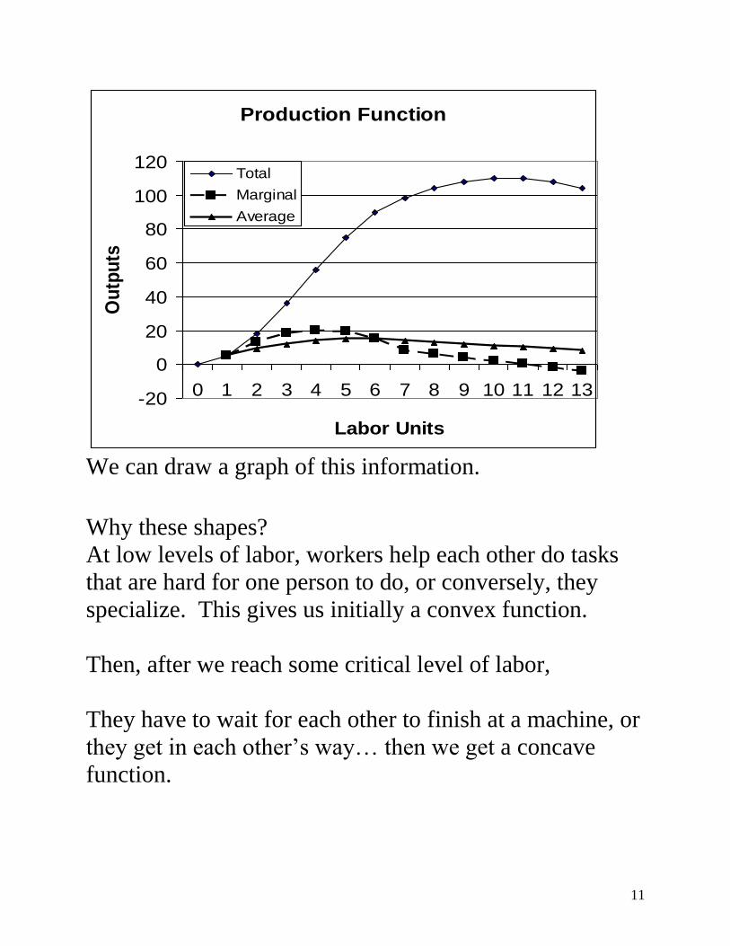
a labor – output table. [fill in units and total first, then revisit marginal and average]

Labor units Total

Output

Marginal

product

Average

product

0 0 NA NA

1 5 5 5

2 18 13 9

3 36 18 12

4 56 20 14

5 75 19 15

6 90 15 15

7 98 8 14

8 104 6 13

9 108 4 12

…

10

Marginal product of Labor: the change in total output

resulting from the use of an additional unit of labor, all

else constant.

L

QMPL

Note that this contrasts with the average product of labor:

the ratio of the output to the number of workers used to

produce this labor.

L

QAPL

Note further that there is also a marginal product of

capital, of materials, of energy… We are focusing on

labor, but other inputs also have marginal and average

measures as we have just defined for labor. [fill these in on chart]

11

Production Function

-20

0

20

40

60

80

100

120

0 1 2 3 4 5 6 7 8 9 10 11 12 13

Labor Units

Ou

tpu

ts

Total

Marginal

Average

We can draw a graph of this information.

Why these shapes?

At low levels of labor, workers help each other do tasks

that are hard for one person to do, or conversely, they

specialize. This gives us initially a convex function.

Then, after we reach some critical level of labor,

They have to wait for each other to finish at a machine, or

they get in each other’s way… then we get a concave

function.

12

If MP curve is above AP curve, then AP is upward

sloping. If MP below AP, then AP downward sloping.

Think of heights for the intuition.

Geometrically, if you draw a ray from the origin to any

point on the Total Product curve, you find the average

product at that point. If you identify the slope of the total

product curve at this point, you find the marginal product.

If AP steeper than MP, then AP > MP. If AP flatter than

MP, then AP < MP. At some point, AP=MP.

The law of diminishing marginal returns. If a firm keeps

increasing an input, holding all other inputs and

technology constant, the corresponding increases in

output will become smaller eventually.

Not diminishing returns, but diminishing marginal

returns.

13

Long run production.

That was a discussion of variation in output due to

different levels of labor holding other things (K, E, M)

constant.

Now, we are in the long run so all inputs are variable.

Note that the short run implies that at least one input is

being held fixed. Do not come away from this with the

impression that the difference between the short run and

the long run is one versus two inputs. That is not right.

In the short run, at least one input and potentially more

than one input is held constant while one or more other

inputs are allowed to vary. In the long run all inputs are

allowed to vary.

However, to keep things simple, we are going to assume

there are only two inputs used in production of our good.

We will call them capital and labor. More than two are

possible (likely) in reality.

We focus on two because it is easier to draw and the logic

carries through to higher dimensions.

We can combine different quantities of these inputs in a

variety of ways to produce a given level of output. Define

14

a curve that traces out the minimum combinations of

inputs required to produce a given level of output.

This is an isoquant. Again, if you want to think of this as

a contour line, it is a contour line on the production

function in 3-D space.

Properties:

1) The farther an isoquant is from the origin, the

greater is the level of output. (remember more is

better than less)

2) Isoquants do not cross, as that would imply

inefficiency. (remember transitivity)

3) Isoquants slope downward, as they are efficient

levels of production (remember there are tradeoffs).

[Draw an isoquant]

15

What will influence the shape of the isoquant?

How substitutable are inputs?

Production function of processed pork.

Processed Pork = pigs bought in New York + pigs bought

in Pennsylvania

Straight line graph

Production function of peanut butter sandwiches.

Peanut butter sandwiches = minimum (dollops of peanut

butter, (slices of bread / 2))

I have 10 dollops of peanut butter, and 4 slices of bread, I

can only make 2 sandwiches.

Leontief graph

Most lie intermediary to these two extreme cases.

Show contrast on single graph, note nature of subs, connect at upper and lower extreme.

16

The slope of the isoquant is called the marginal rate of

technical substitution.

This tells us the trade off between inputs in production. It

is measured as the number of units of one input that have

to be given up while increasing the other input to continue

to produce a given level of output.

The MRTS, like the MRS, is a negative number since it is

implicitly a trade-off. Here, we define it for the capital to

labor MRTS.

L

K

laborchange

capitalchangeMRTSKL

Unless goods are perfect substitutes (MRTS=-1) or

perfect complements (MRTS=-∞/ undefined, or 0), the

MRTS varies as different points are considered on the

isoquant.

17

Remember we are on an isoquant. The quantity of output

stays the same. Therefore, we know that if we change

labor and change capital on a given isoquant, the total

output should not change.

Recall that K

TPMPK

, and a similar expression

exists for the marginal product of labor.

So if we know the change in total product is zero by

definition, and we know the definition of the marginal

product is what we just saw, we can add zero plus zero to

find the following.

0TPMPLMPK LK

Show math, note connection to calculus, and answer zero minus zero question if it comes up.

Also note connection back to MRS and the Marginal Utility equations developed earlier.

While not overwhelming exciting, this allows us to gain

the insight that the marginal rate of technical substitution

is equal to the negative of the ratio of the marginal

products (important: note the numerator – denominator

relationship).

K

LKL

MP

MP

L

KMRTS

18

From an intuitive point of view, the movement along an

isoquant is related to marginal changes.

I am getting this level of output using a specific mix of

inputs, now I want to move over there to another mix of

inputs holding output constant.

That is a marginal change.

19

Returns to scale.

Up until now, we have been considering adjustments to

our input bundles, holding output constant. That is how

we have defined an isoquant. Or we have been changing

one input at a time, holding others constant. That is how

we thought about a production function.

Now, however, we want to turn to the question of how

changes in the total input bundle are related to changes in

output.

What can we learn by comparing different isoquants

rather than looking at movement along a given isoquant?

We are going to look at a specific type of change to the

input bundle – blowups. Equal percentage change applied

to all inputs.

I use labor and capital to produce my good. Let’s say we

can continue to ignore other inputs like materials and

energy for production of our good.

What are the implications of different production

functions for changing input levels?

20

Say I use 2 units of labor and 3 units of capital to produce

6 problem sets. In this case, assume the production

function is defined by capital times labor. If I double both

units (4 units of labor and 6 units of capital) I get 24 units

of problem sets.

2*3=6

new output= (2*2)*(3*2)=4*(2*3)=4*6=24

Doubling inputs gives a four-fold increase in output.

(24/6)=4

Increasing Returns to scale. Doubling inputs leads to a

more than double increase in outputs.

f(2*K,2*L) > 2*f(K,L)

21

Say instead that the production function is capital plus

labor (perfect substitutes in production).

2+3=5

new output=(2*2)+(2*3)=2*(2+3)=10

Doubling inputs gives a doubling of output.

(10/5)=2

Constant returns to scale. Case two (additive production

function). Doubling inputs leads to a doubling of output.

f(2*K,2*L) = 2*f(K,L)

Finally, assume we have a production function that

defines output as the natural log of capital times labor.

ln(2*3)=1.79

New output = ln((2*2)*(2*3))=ln(4*6)=3.18

Doubling inputs increases output by 78%

(3.18/1.79)=1.78

Decreasing returns to scale. Doubling inputs leads to a

less than double increase in output.

f(2*K,2*L) < 2*f(K,L)

22

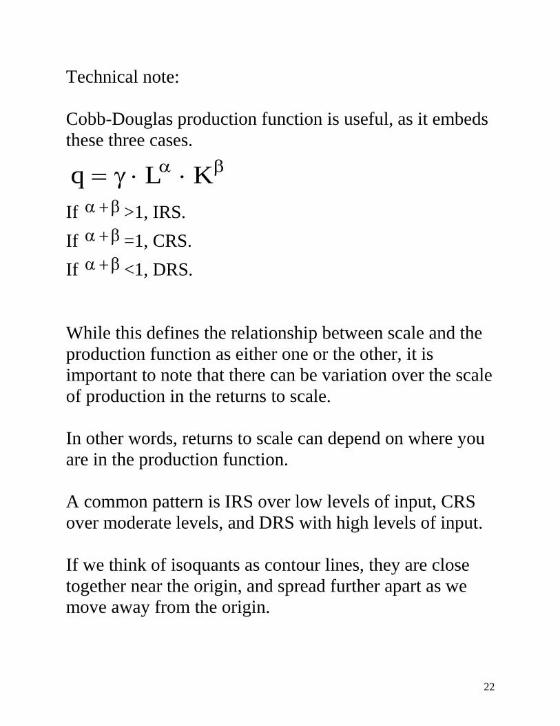
Technical note:

Cobb-Douglas production function is useful, as it embeds

these three cases.

KLq

If >1, IRS.

If =1, CRS.

If <1, DRS.

While this defines the relationship between scale and the

production function as either one or the other, it is

important to note that there can be variation over the scale

of production in the returns to scale.

In other words, returns to scale can depend on where you

are in the production function.

A common pattern is IRS over low levels of input, CRS

over moderate levels, and DRS with high levels of input.

If we think of isoquants as contour lines, they are close

together near the origin, and spread further apart as we

move away from the origin.

23

Show graph from book that illustrates IRS over low ranges, CRS mid range, and DRS higher

range.

Innovations.

Technological progress is one of the main driving factors

of economic growth.

Different types:

Neutral technical change. All inputs are equally affected.

Allows same input bundle to be used, but generates more

output.

Nonneutral technical change. The innovation affects

inputs unequally. This alters the proportions of the input

bundles when generating more output.