chapter 6 external economies and monopolistic competition - spot

1

Chapter 6

External Economies and Monopolistic Competition

Now we continue our study of increasing returns to scale, turning to models based onexternal economies of scale and monopolistic-competition models. I have grouped these twotogether in one chapter since there are close technical similarities between them. A formaldemonstration of this equivalence is found in Markusen (CJE vol. 23, 1990, 495-508.).

These models require a few tricks to code in MPS/GE, because MPS/GE requires allactivities to have constant returns to scale. Because of this, I want to present MCP versions ofthe models first, in order to show clearly what equations and inequalities are being solved. ThenI present the MPS/GE versions and show the tricks. In very simple models such as the onespresented here, it is generally easiest to stick with the MCP solver and not use the higher-levellanguage. But it more complicated higher-dimension models, it is best to learn the tricks and useMPS/GE.

Models are as follows:

M61-MCP.GMS Closed economy external economies of scale, MCP version

M61-MPS.GMS Closed economy external economies of scale, MPS/GE version

M62-MCP.GMS Closed economy large-group monopolistic competition, MCP version

M62-MPS.GMS Closed economy large-group monopolistic competition, MPS/GE verion

M63-MPC.GMS Two-country model with large-group monopolistic competition, MCPversion

M63-MPC.GMS Two-country model with large-group monopolistic competition, MPS/GEversion

2

Model 61-MCP Closed economy external economies of scale, MCP version

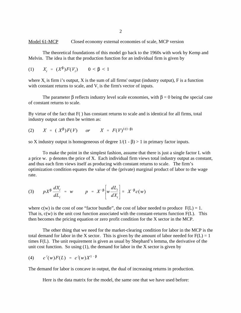
The theoretical foundations of this model go back to the 1960s with work by Kemp andMelvin. The idea is that the production function for an individual firm is given by

(1)

where Xi is firm i’s output, X is the sum of all firms' output (industry output), F is a functionwith constant returns to scale, and Vi is the firm's vector of inputs.

The parameter β reflects industry level scale economies, with β = 0 being the special caseof constant returns to scale.

By virtue of the fact that F( ) has constant returns to scale and is identical for all firms, totalindustry output can then be written as:

(2)

so X industry output is homogeneous of degree 1/(1 - β) > 1 in primary factor inputs.

To make the point in the simplest fashion, assume that there is just a single factor L witha price w. p denotes the price of X. Each individual firm views total industry output as constant,and thus each firm views itself as producing with constant returns to scale. The firm’soptimization condition equates the value of the (private) marginal product of labor to the wagerate.

(3)

where c(w) is the cost of one “factor bundle”, the cost of labor needed to produce F(L) = 1. That is, c(w) is the unit cost function associated with the constant-returns function F(L). Thisthen becomes the pricing equation or zero profit condition for the X sector in the MCP.

The other thing that we need for the market-clearing condition for labor in the MCP is thetotal demand for labor in the X sector. This is given by the amount of labor needed for F(L) = 1times F(L). The unit requirement is given as usual by Shephard’s lemma, the derivative of theunit cost function. So using (1), the demand for labor in the X sector is given by

(4)

The demand for labor is concave in output, the dual of increasing returns in production.

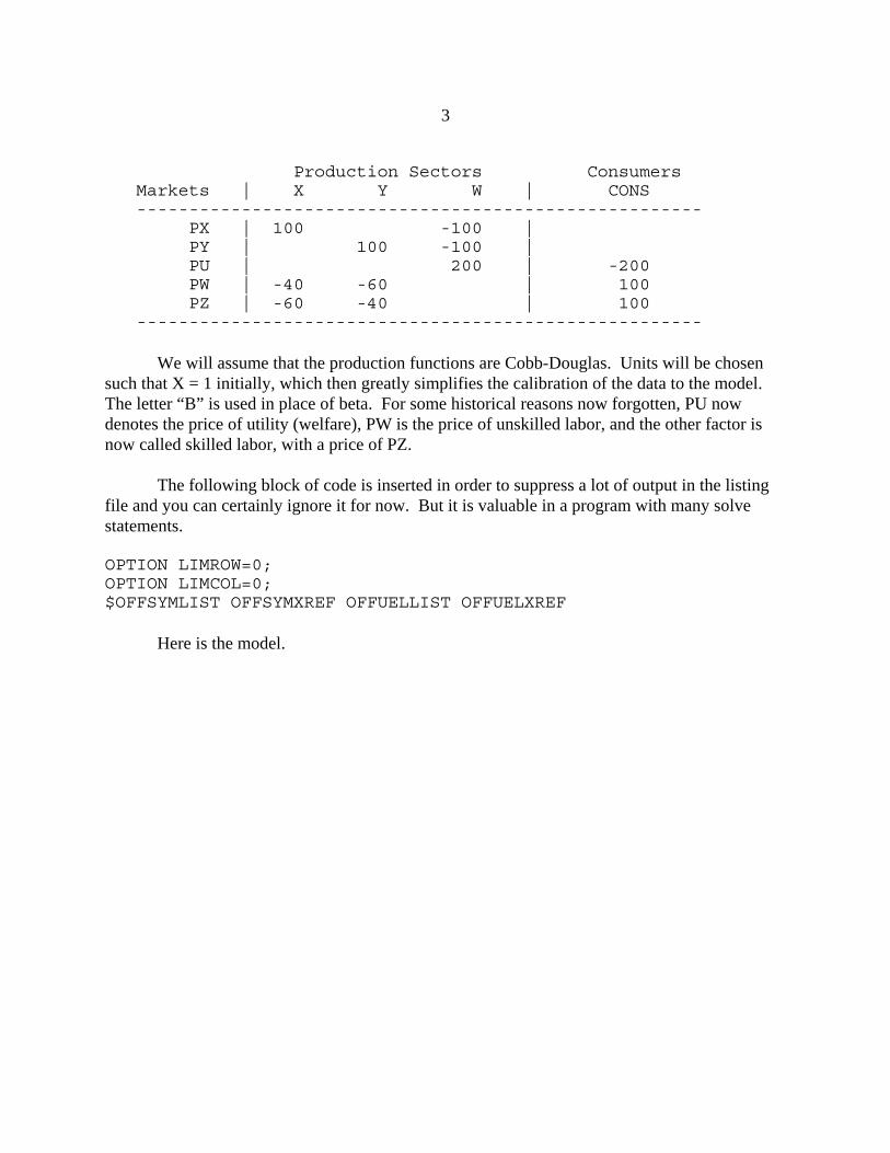
Here is the data matrix for the model, the same one that we have used before:

3

Production Sectors Consumers Markets | X Y W | CONS ------------------------------------------------------ PX | 100 -100 | PY | 100 -100 | PU | 200 | -200 PW | -40 -60 | 100 PZ | -60 -40 | 100 ------------------------------------------------------

We will assume that the production functions are Cobb-Douglas. Units will be chosensuch that X = 1 initially, which then greatly simplifies the calibration of the data to the model. The letter “B” is used in place of beta. For some historical reasons now forgotten, PU nowdenotes the price of utility (welfare), PW is the price of unskilled labor, and the other factor isnow called skilled labor, with a price of PZ.

The following block of code is inserted in order to suppress a lot of output in the listingfile and you can certainly ignore it for now. But it is valuable in a program with many solvestatements.

OPTION LIMROW=0;OPTION LIMCOL=0;$OFFSYMLIST OFFSYMXREF OFFUELLIST OFFUELXREF

Here is the model.

4

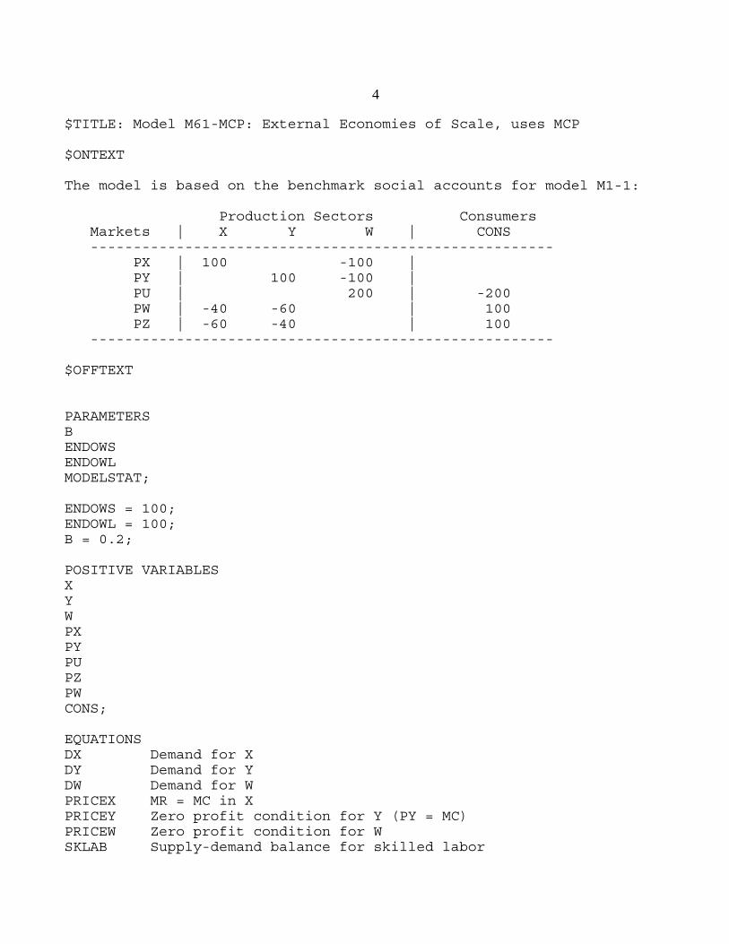
$TITLE: Model M61-MCP: External Economies of Scale, uses MCP

$ONTEXT

The model is based on the benchmark social accounts for model M1-1:


$OFFTEXT

PARAMETERSBENDOWSENDOWLMODELSTAT;

ENDOWS = 100;ENDOWL = 100;B = 0.2;

POSITIVE VARIABLESXYWPXPYPUPZPWCONS;

EQUATIONSDX Demand for XDY Demand for YDW Demand for WPRICEX MR = MC in XPRICEY Zero profit condition for Y (PY = MC)PRICEW Zero profit condition for WSKLAB Supply-demand balance for skilled labor

5

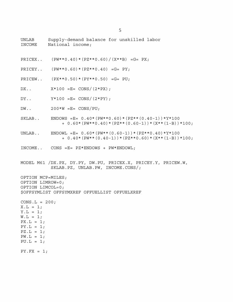
UNLAB Supply-demand balance for unskilled labor INCOME National income;

PRICEX.. (PW**0.40)*(PZ**0.60)/(X**B) =G= PX;

PRICEY.. (PW**0.60)*(PZ**0.40) =G= PY;

PRICEW.. (PX**0.50)*(PY**0.50) =G= PU;

DX.. X*100 =E= CONS/(2*PX);

DY.. Y*100 =E= CONS/(2*PY);

DW.. 200*W =E= CONS/PU;

SKLAB.. ENDOWS =E= 0.40*(PW**0.60)*(PZ**(0.40-1))*Y*100 + 0.60*(PW**0.40)*(PZ**(0.60-1))*(X**(1-B))*100; UNLAB.. ENDOWL =E= 0.60*(PW**(0.60-1))*(PZ**0.40)*Y*100 + 0.40*(PW**(0.40-1))*(PZ**0.60)*(X**(1-B))*100; INCOME.. CONS =E= PZ*ENDOWS + PW*ENDOWL;

MODEL M61 /DX.PX, DY.PY, DW.PU, PRICEX.X, PRICEY.Y, PRICEW.W, SKLAB.PZ, UNLAB.PW, INCOME.CONS/;

OPTION MCP=MILES;OPTION LIMROW=0;OPTION LIMCOL=0;$OFFSYMLIST OFFSYMXREF OFFUELLIST OFFUELXREF CONS.L = 200;X.L = 1;Y.L = 1;W.L = 1;PX.L = 1;PY.L = 1;PZ.L = 1;PW.L = 1;PU.L = 1;

PY.FX = 1;

6

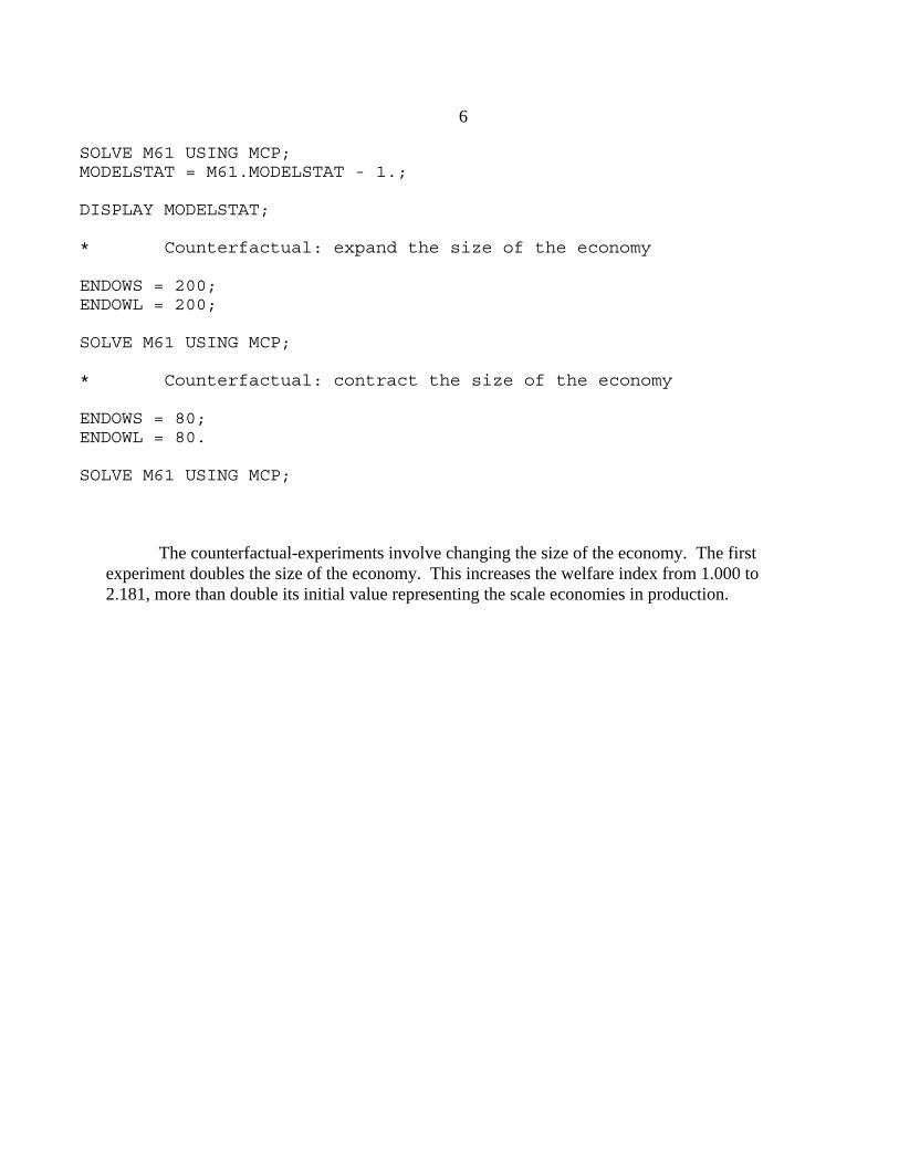
SOLVE M61 USING MCP;MODELSTAT = M61.MODELSTAT - 1.;

DISPLAY MODELSTAT;

* Counterfactual: expand the size of the economy

ENDOWS = 200;ENDOWL = 200;

SOLVE M61 USING MCP;

* Counterfactual: contract the size of the economy

ENDOWS = 80;ENDOWL = 80.


The counterfactual-experiments involve changing the size of the economy. The firstexperiment doubles the size of the economy. This increases the welfare index from 1.000 to2.181, more than double its initial value representing the scale economies in production.

7

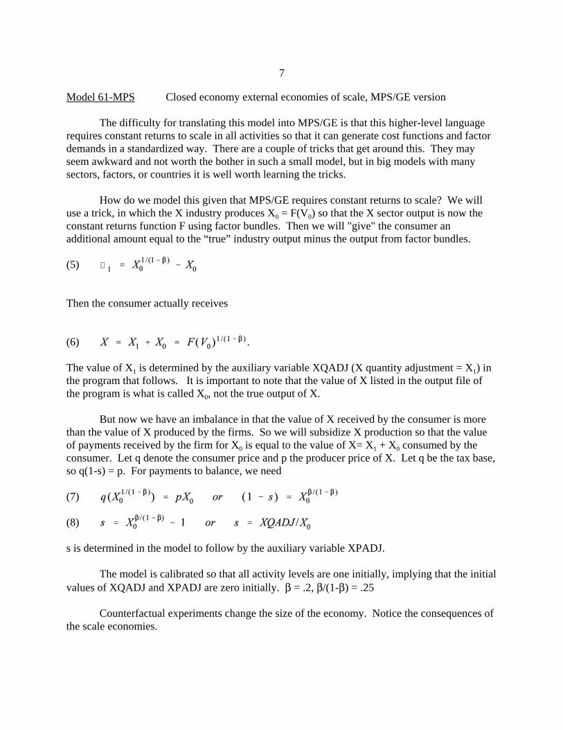
Model 61-MPS Closed economy external economies of scale, MPS/GE version

The difficulty for translating this model into MPS/GE is that this higher-level languagerequires constant returns to scale in all activities so that it can generate cost functions and factordemands in a standardized way. There are a couple of tricks that get around this. They mayseem awkward and not worth the bother in such a small model, but in big models with manysectors, factors, or countries it is well worth learning the tricks.

How do we model this given that MPS/GE requires constant returns to scale? We willuse a trick, in which the X industry produces X0 = F(V0) so that the X sector output is now theconstant returns function F using factor bundles. Then we will "give" the consumer anadditional amount equal to the “true” industry output minus the output from factor bundles.

(5)

Then the consumer actually receives

(6) .

The value of X1 is determined by the auxiliary variable XQADJ (X quantity adjustment = X1) inthe program that follows. It is important to note that the value of X listed in the output file ofthe program is what is called X0, not the true output of X.

But now we have an imbalance in that the value of X received by the consumer is morethan the value of X produced by the firms. So we will subsidize X production so that the valueof payments received by the firm for X0 is equal to the value of X= X1 + X0 consumed by theconsumer. Let q denote the consumer price and p the producer price of X. Let q be the tax base,so q(1-s) = p. For payments to balance, we need

(7)

(8)

s is determined in the model to follow by the auxiliary variable XPADJ.

The model is calibrated so that all activity levels are one initially, implying that the initialvalues of XQADJ and XPADJ are zero initially. β = .2, β/(1-β) = .25

Counterfactual experiments change the size of the economy. Notice the consequences ofthe scale economies.

8

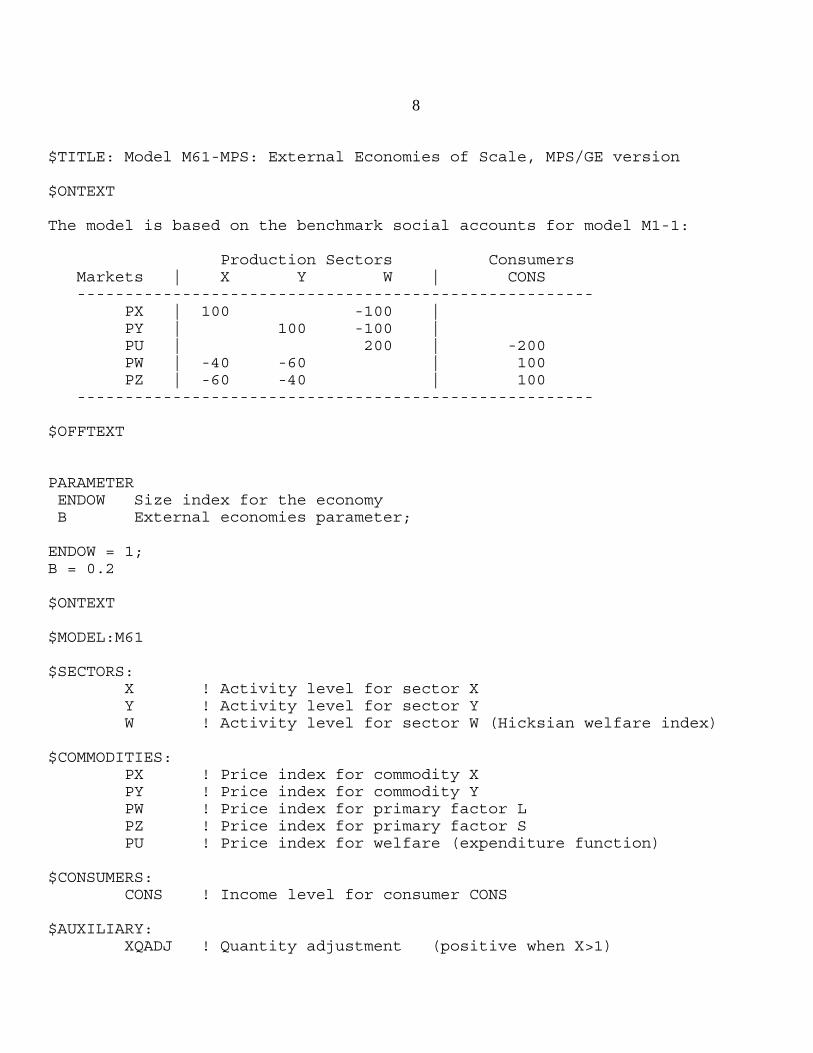
$TITLE: Model M61-MPS: External Economies of Scale, MPS/GE version

$ONTEXT

The model is based on the benchmark social accounts for model M1-1:


$OFFTEXT

PARAMETER ENDOW Size index for the economy B External economies parameter;

ENDOW = 1;B = 0.2

$ONTEXT

$MODEL:M61

$SECTORS: X ! Activity level for sector X Y ! Activity level for sector Y W ! Activity level for sector W (Hicksian welfare index)

$COMMODITIES: PX ! Price index for commodity X PY ! Price index for commodity Y PW ! Price index for primary factor L PZ ! Price index for primary factor S PU ! Price index for welfare (expenditure function)

$CONSUMERS: CONS ! Income level for consumer CONS

$AUXILIARY: XQADJ ! Quantity adjustment (positive when X>1)

9

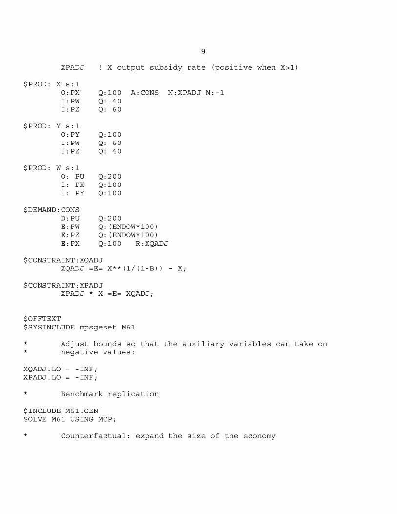
XPADJ ! X output subsidy rate (positive when X>1)

$PROD: X s:1 O:PX Q:100 A:CONS N:XPADJ M:-1 I:PW Q: 40 I:PZ Q: 60

$PROD: Y s:1 O:PY Q:100 I:PW Q: 60 I:PZ Q: 40

$PROD: W s:1 O: PU Q:200 I: PX Q:100 I: PY Q:100

$DEMAND:CONS D:PU Q:200 E:PW Q:(ENDOW*100) E:PZ Q:(ENDOW*100) E:PX Q:100 R:XQADJ

$CONSTRAINT:XQADJ XQADJ =E= X**(1/(1-B)) - X;

$CONSTRAINT:XPADJ XPADJ * X =E= XQADJ;

$OFFTEXT$SYSINCLUDE mpsgeset M61

* Adjust bounds so that the auxiliary variables can take on * negative values:

XQADJ.LO = -INF;XPADJ.LO = -INF;

* Benchmark replication

$INCLUDE M61.GENSOLVE M61 USING MCP;


10

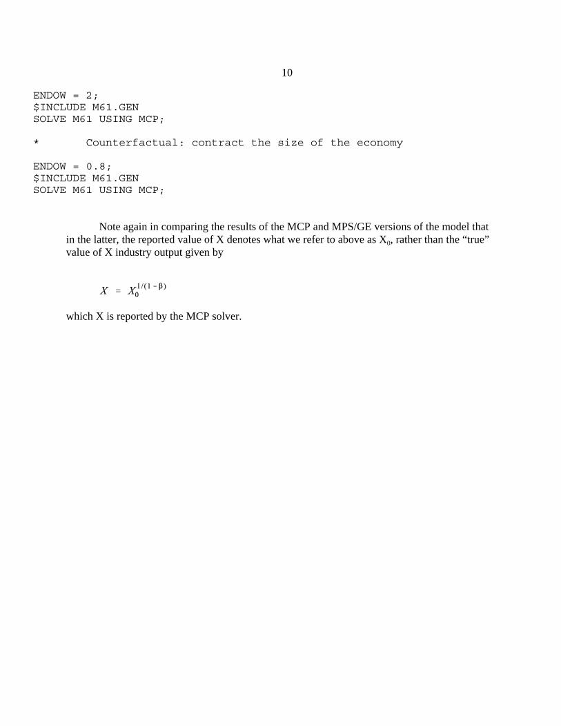
ENDOW = 2;$INCLUDE M61.GENSOLVE M61 USING MCP;

* Counterfactual: contract the size of the economy

ENDOW = 0.8;$INCLUDE M61.GENSOLVE M61 USING MCP;

Note again in comparing the results of the MCP and MPS/GE versions of the model thatin the latter, the reported value of X denotes what we refer to above as X0, rather than the “true”value of X industry output given by

which X is reported by the MCP solver.

11

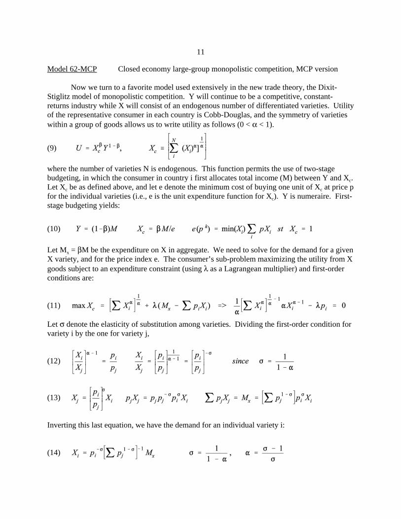
Model 62-MCP Closed economy large-group monopolistic competition, MCP version

Now we turn to a favorite model used extensively in the new trade theory, the Dixit-Stiglitz model of monopolistic competition. Y will continue to be a competitive, constant-returns industry while X will consist of an endogenous number of differentiated varieties. Utilityof the representative consumer in each country is Cobb-Douglas, and the symmetry of varietieswithin a group of goods allows us to write utility as follows (0 < α < 1).

(9)

where the number of varieties N is endogenous. This function permits the use of two-stagebudgeting, in which the consumer in country i first allocates total income (M) between Y and Xc. Let Xc be as defined above, and let e denote the minimum cost of buying one unit of Xc at price pfor the individual varieties (i.e., e is the unit expenditure function for Xc). Y is numeraire. First-stage budgeting yields:

(10)

Let Mx = βM be the expenditure on X in aggregate. We need to solve for the demand for a givenX variety, and for the price index e. The consumer’s sub-problem maximizing the utility from Xgoods subject to an expenditure constraint (using λ as a Lagrangean multiplier) and first-orderconditions are:

(11)

Let σ denote the elasticity of substitution among varieties. Dividing the first-order condition forvariety i by the one for variety j,

(12)

(13)

Inverting this last equation, we have the demand for an individual variety i:

(14)

12

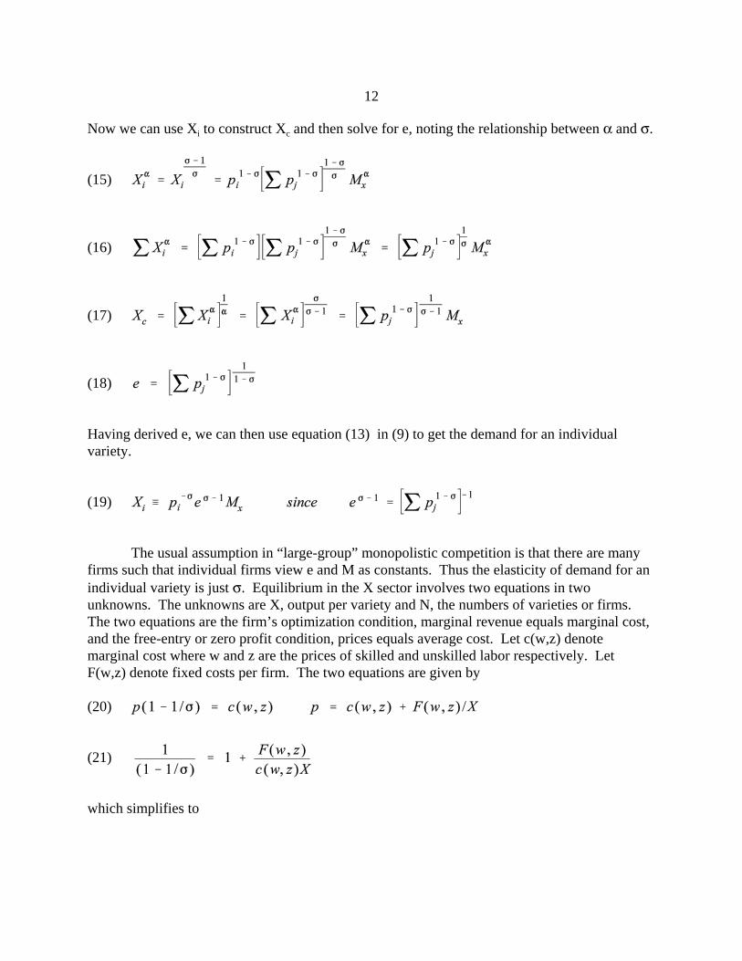
Now we can use Xi to construct Xc and then solve for e, noting the relationship between α and σ.

(15)

(16)

(17)

(18)

Having derived e, we can then use equation (13) in (9) to get the demand for an individualvariety.

(19)

The usual assumption in “large-group” monopolistic competition is that there are manyfirms such that individual firms view e and M as constants. Thus the elasticity of demand for anindividual variety is just σ. Equilibrium in the X sector involves two equations in twounknowns. The unknowns are X, output per variety and N, the numbers of varieties or firms. The two equations are the firm’s optimization condition, marginal revenue equals marginal cost,and the free-entry or zero profit condition, prices equals average cost. Let c(w,z) denotemarginal cost where w and z are the prices of skilled and unskilled labor respectively. LetF(w,z) denote fixed costs per firm. The two equations are given by

(20)

(21)

which simplifies to

13

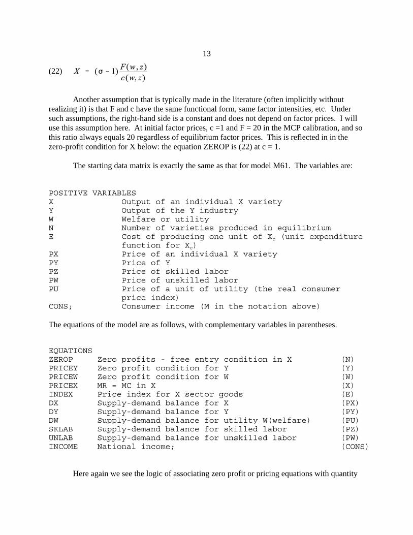
(22)

Another assumption that is typically made in the literature (often implicitly withoutrealizing it) is that F and c have the same functional form, same factor intensities, etc. Undersuch assumptions, the right-hand side is a constant and does not depend on factor prices. I willuse this assumption here. At initial factor prices, c =1 and F = 20 in the MCP calibration, and sothis ratio always equals 20 regardless of equilibrium factor prices. This is reflected in in thezero-profit condition for X below: the equation ZEROP is (22) at c = 1.

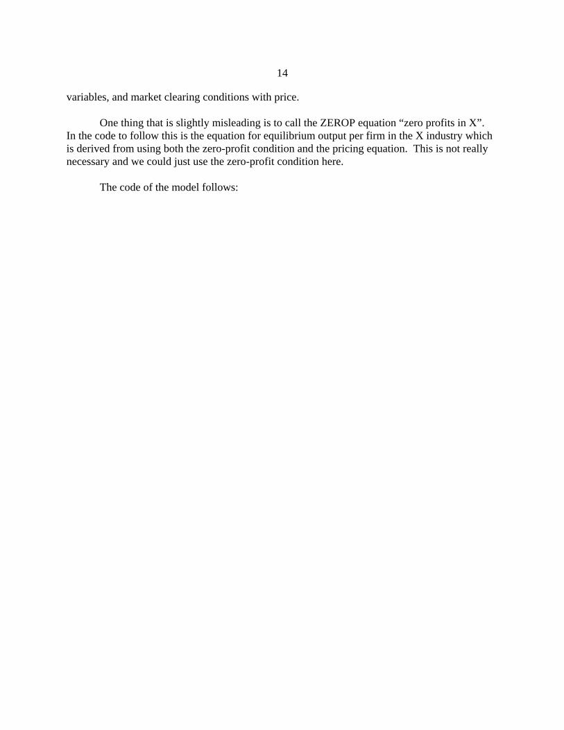
The starting data matrix is exactly the same as that for model M61. The variables are:

POSITIVE VARIABLES X Output of an individual X varietyY Output of the Y industryW Welfare or utilityN Number of varieties produced in equilibriumE Cost of producing one unit of Xc (unit expenditure

function for Xc)PX Price of an individual X varietyPY Price of YPZ Price of skilled laborPW Price of unskilled laborPU Price of a unit of utility (the real consumer

price index)CONS; Consumer income (M in the notation above)

The equations of the model are as follows, with complementary variables in parentheses.

EQUATIONSZEROP Zero profits - free entry condition in X (N)PRICEY Zero profit condition for Y (Y)PRICEW Zero profit condition for W (W)PRICEX MR = MC in X (X)INDEX Price index for X sector goods (E)DX Supply-demand balance for X (PX)DY Supply-demand balance for Y (PY)DW Supply-demand balance for utility W(welfare) (PU)SKLAB Supply-demand balance for skilled labor (PZ)UNLAB Supply-demand balance for unskilled labor (PW)INCOME National income; (CONS)

Here again we see the logic of associating zero profit or pricing equations with quantity

14

variables, and market clearing conditions with price.

One thing that is slightly misleading is to call the ZEROP equation “zero profits in X”. In the code to follow this is the equation for equilibrium output per firm in the X industry whichis derived from using both the zero-profit condition and the pricing equation. This is not reallynecessary and we could just use the zero-profit condition here.

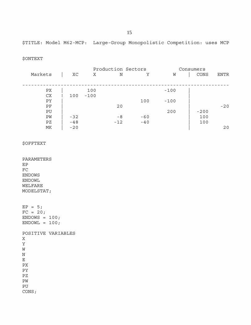
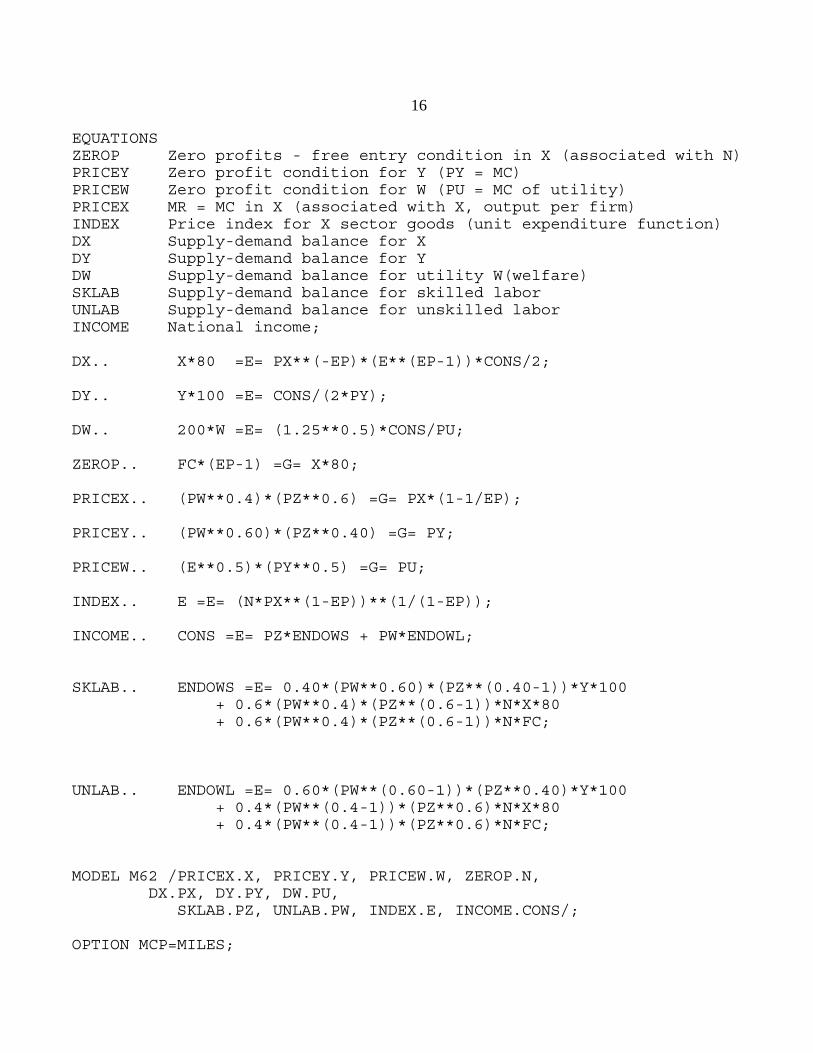
The code of the model follows:

15

$TITLE: Model M62-MCP: Large-Group Monopolistic Competition: uses MCP

$ONTEXT

Production Sectors Consumers Markets | XC X N Y W | CONS ENTR ---------------------------------------------------------------------- PX | 100 -100 | CX ! 100 -100 | PY | 100 -100 | PF | 20 | -20 PU | 200 | -200 PW | -32 -8 -60 | 100 PZ | -48 -12 -40 | 100 MK | -20 | 20

$OFFTEXT

PARAMETERSEPFCENDOWSENDOWLWELFAREMODELSTAT;

EP = 5;FC = 20;ENDOWS = 100;ENDOWL = 100;

POSITIVE VARIABLES XYWNEPXPYPZPWPUCONS;

16

EQUATIONSZEROP Zero profits - free entry condition in X (associated with N)PRICEY Zero profit condition for Y (PY = MC)PRICEW Zero profit condition for W (PU = MC of utility)PRICEX MR = MC in X (associated with X, output per firm)INDEX Price index for X sector goods (unit expenditure function)DX Supply-demand balance for XDY Supply-demand balance for YDW Supply-demand balance for utility W(welfare)SKLAB Supply-demand balance for skilled laborUNLAB Supply-demand balance for unskilled labor INCOME National income;

DX.. X*80 =E= PX**(-EP)*(E**(EP-1))*CONS/2;

DY.. Y*100 =E= CONS/(2*PY);

DW.. 200*W =E= (1.25**0.5)*CONS/PU;

ZEROP.. FC*(EP-1) =G= X*80;

PRICEX.. (PW**0.4)*(PZ**0.6) =G= PX*(1-1/EP);

PRICEY.. (PW**0.60)*(PZ**0.40) =G= PY;

PRICEW.. (E**0.5)*(PY**0.5) =G= PU;

INDEX.. E =E= (N*PX**(1-EP))**(1/(1-EP));

INCOME.. CONS =E= PZ*ENDOWS + PW*ENDOWL;

SKLAB.. ENDOWS =E= 0.40*(PW**0.60)*(PZ**(0.40-1))*Y*100 + 0.6*(PW**0.4)*(PZ**(0.6-1))*N*X*80 + 0.6*(PW**0.4)*(PZ**(0.6-1))*N*FC;

UNLAB.. ENDOWL =E= 0.60*(PW**(0.60-1))*(PZ**0.40)*Y*100 + 0.4*(PW**(0.4-1))*(PZ**0.6)*N*X*80 + 0.4*(PW**(0.4-1))*(PZ**0.6)*N*FC;

MODEL M62 /PRICEX.X, PRICEY.Y, PRICEW.W, ZEROP.N, DX.PX, DY.PY, DW.PU,

SKLAB.PZ, UNLAB.PW, INDEX.E, INCOME.CONS/;

OPTION MCP=MILES;

17

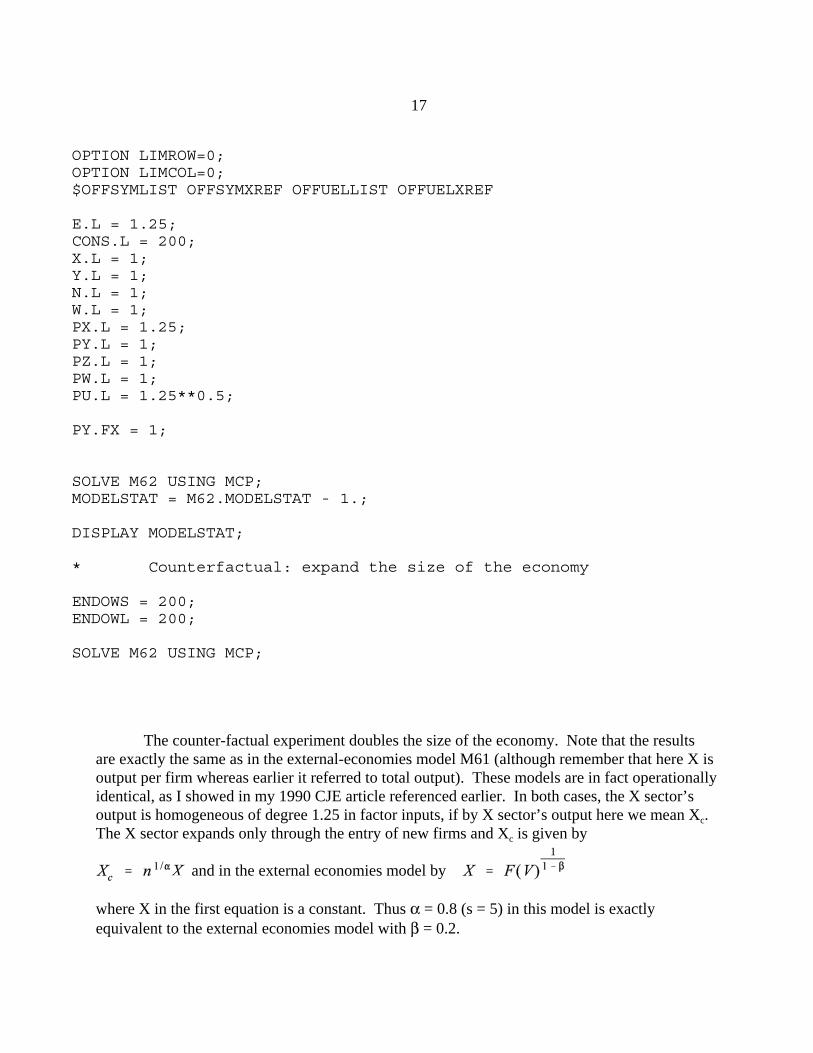
OPTION LIMROW=0;OPTION LIMCOL=0;$OFFSYMLIST OFFSYMXREF OFFUELLIST OFFUELXREF

E.L = 1.25; CONS.L = 200;X.L = 1;Y.L = 1;N.L = 1;W.L = 1;PX.L = 1.25;PY.L = 1;PZ.L = 1;PW.L = 1;PU.L = 1.25**0.5;

PY.FX = 1;


DISPLAY MODELSTAT;


ENDOWS = 200;ENDOWL = 200;


The counter-factual experiment doubles the size of the economy. Note that the resultsare exactly the same as in the external-economies model M61 (although remember that here X isoutput per firm whereas earlier it referred to total output). These models are in fact operationallyidentical, as I showed in my 1990 CJE article referenced earlier. In both cases, the X sector’soutput is homogeneous of degree 1.25 in factor inputs, if by X sector’s output here we mean Xc.The X sector expands only through the entry of new firms and Xc is given by

and in the external economies model by

where X in the first equation is a constant. Thus α = 0.8 (s = 5) in this model is exactlyequivalent to the external economies model with β = 0.2.

18

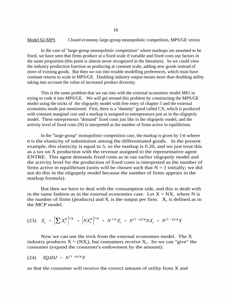
Model 62-MPS Closed economy large-group monopolistic competition, MPS/GE verion

In the case of "large-group monopolistic competition" where markups are assumed to befixed, we have seen that firms produce at a fixed scale if variable and fixed costs use factors inthe same proportion (this point is almost never recognized in the literature). So we could viewthe industry production function as producing at constant scale, adding new goods instead ofmore of existing goods. But then we run into trouble modelling preferences, which must haveconstant returns to scale in MPS/GE. Doubling industry output means more than doubling utilitytaking into account the value of increased product diversity.

This is the same problem that we ran into with the external economies model M61 intrying to code it into MPS/GE. We will get around this problem by constructing the MPS/GEmodel using the tricks of the oligopoly model with free entry of chapter 5 and the externaleconomies mode just mentioned. First, there is a "dummy" good called CX, which is producedwith constant marginal cost and a markup is assigned to entrepreneurs just as in the oligopolymodel. These entrepreneurs "demand" fixed costs just like in the oligopoly model, and theactivity level of fixed costs (N) is interpreted as the number of firms active in equilibrium.

In the "large-group" monopolistic-competition case, the markup is given by 1/σ whereσ is the elasticity of substitution among the differentiated goods. In the presentexample, this elasticity is equal to 5, so the markup is 0.20, and we just treat thisas a tax on X production with the revenue assigned to the representative agentENTRE. This agent demands fixed costs as in our earlier oligopoly model andthe activity level for the production of fixed costs is interpreted as the number offirms active in equilibrium (units will be chosen such that N = 1 initially; we didnot do this in the oligopoly model because the number of firms appears in themarkup formula).

But then we have to deal with the consumption side, and this is dealt within the same fashion as in the external economies case. Let X = NXi where N isthe number of firms (products) and Xi is the output per firm. Xc is defined as inthe MCP model.

(23)

Now we can use the trick from the external economies model. The Xindustry produces X = (NXi), but consumers receive Xc. So we can "give" theconsumer (expand the consumer's endowment by the amount):

(24)

so that the consumer will receive the correct amount of utility from X and

19

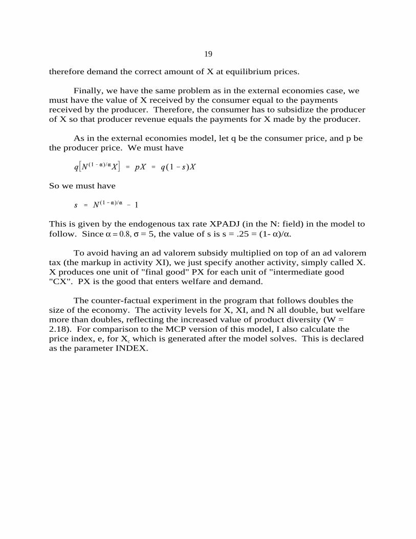
therefore demand the correct amount of X at equilibrium prices.

Finally, we have the same problem as in the external economies case, wemust have the value of X received by the consumer equal to the paymentsreceived by the producer. Therefore, the consumer has to subsidize the producerof X so that producer revenue equals the payments for X made by the producer.

As in the external economies model, let q be the consumer price, and p bethe producer price. We must have

So we must have

This is given by the endogenous tax rate XPADJ (in the N: field) in the model tofollow. Since α = 0.8, σ = 5, the value of s is s = .25 = (1- α)/α.

To avoid having an ad valorem subsidy multiplied on top of an ad valoremtax (the markup in activity XI), we just specify another activity, simply called X. X produces one unit of "final good" PX for each unit of "intermediate good"CX". PX is the good that enters welfare and demand.

The counter-factual experiment in the program that follows doubles thesize of the economy. The activity levels for X, XI, and N all double, but welfaremore than doubles, reflecting the increased value of product diversity (W =2.18). For comparison to the MCP version of this model, I also calculate theprice index, e, for Xc which is generated after the model solves. This is declaredas the parameter INDEX.

20

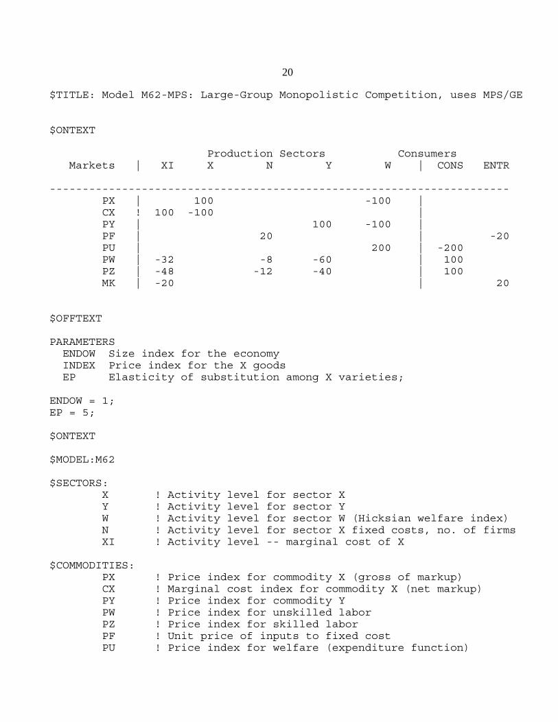
$TITLE: Model M62-MPS: Large-Group Monopolistic Competition, uses MPS/GE

$ONTEXT

Production Sectors Consumers Markets | XI X N Y W | CONS ENTR ---------------------------------------------------------------------- PX | 100 -100 | CX ! 100 -100 | PY | 100 -100 | PF | 20 | -20 PU | 200 | -200 PW | -32 -8 -60 | 100 PZ | -48 -12 -40 | 100 MK | -20 | 20

$OFFTEXT

PARAMETERS ENDOW Size index for the economy INDEX Price index for the X goods EP Elasticity of substitution among X varieties;

ENDOW = 1;EP = 5;

$ONTEXT

$MODEL:M62

$SECTORS: X ! Activity level for sector X Y ! Activity level for sector Y W ! Activity level for sector W (Hicksian welfare index) N ! Activity level for sector X fixed costs, no. of firms XI ! Activity level -- marginal cost of X

$COMMODITIES: PX ! Price index for commodity X (gross of markup) CX ! Marginal cost index for commodity X (net markup) PY ! Price index for commodity Y PW ! Price index for unskilled labor PZ ! Price index for skilled labor PF ! Unit price of inputs to fixed cost PU ! Price index for welfare (expenditure function)

21

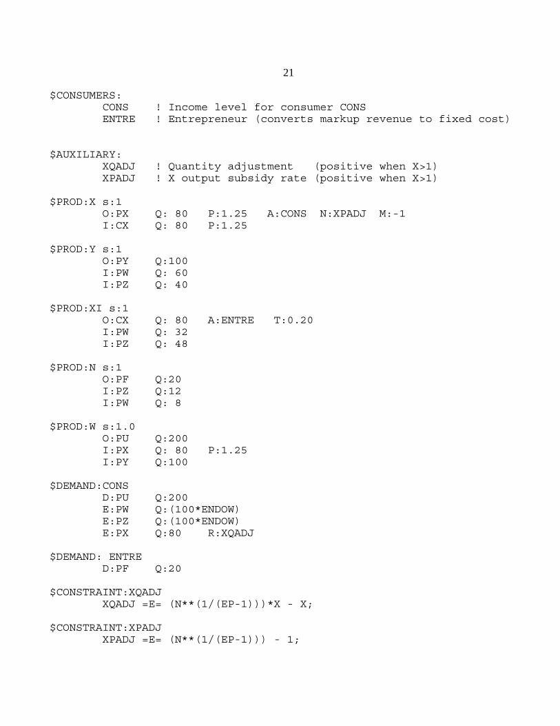
$CONSUMERS: CONS ! Income level for consumer CONS ENTRE ! Entrepreneur (converts markup revenue to fixed cost)

$AUXILIARY: XQADJ ! Quantity adjustment (positive when X>1) XPADJ ! X output subsidy rate (positive when X>1)

$PROD:X s:1 O:PX Q: 80 P:1.25 A:CONS N:XPADJ M:-1 I:CX Q: 80 P:1.25

$PROD:Y s:1 O:PY Q:100 I:PW Q: 60 I:PZ Q: 40

$PROD:XI s:1 O:CX Q: 80 A:ENTRE T:0.20 I:PW Q: 32 I:PZ Q: 48

$PROD:N s:1 O:PF Q:20 I:PZ Q:12 I:PW Q: 8

$PROD:W s:1.0 O:PU Q:200 I:PX Q: 80 P:1.25 I:PY Q:100

$DEMAND:CONS D:PU Q:200 E:PW Q:(100*ENDOW) E:PZ Q:(100*ENDOW) E:PX Q:80 R:XQADJ

$DEMAND: ENTRE D:PF Q:20

$CONSTRAINT:XQADJ XQADJ =E= (N**(1/(EP-1)))*X - X;

$CONSTRAINT:XPADJ XPADJ =E= (N**(1/(EP-1))) - 1;

22

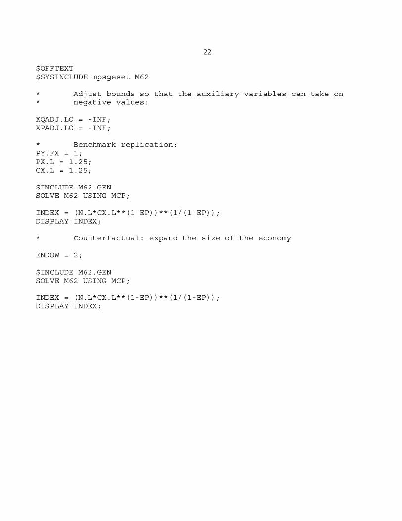
$OFFTEXT$SYSINCLUDE mpsgeset M62

* Adjust bounds so that the auxiliary variables can take on * negative values:

XQADJ.LO = -INF;XPADJ.LO = -INF;

* Benchmark replication:PY.FX = 1;PX.L = 1.25; CX.L = 1.25;


INDEX = (N.L*CX.L**(1-EP))**(1/(1-EP));DISPLAY INDEX;


ENDOW = 2;


INDEX = (N.L*CX.L**(1-EP))**(1/(1-EP));DISPLAY INDEX;

23

Model M63-MCP Two-country model with large-group monopolistic competition, MCPversion

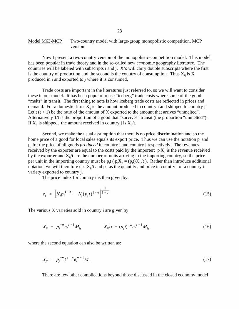
Now I present a two-country version of the monopolistic-competition model. This modelhas been popular in trade theory and in the so-called new economic geography literature. Thecountries will be labeled with subscripts i and j. X’s will carry double subscripts where the firstis the country of production and the second is the country of consumption. Thus Xij is Xproduced in i and exported to j where it is consumed.

Trade costs are important in the literatures just referred to, so we will want to considerthese in our model. It has been popular to use “iceberg” trade costs where some of the good“melts” in transit. The first thing to note is how iceberg trade costs are reflected in prices anddemand. For a domestic firm, Xij is the amount produced in country i and shipped to country j.Let t (t > 1) be the ratio of the amount of X exported to the amount that arrives “unmelted”. Alternatively 1/t is the proportion of a good that “survives” transit (the proportion “unmelted”). If Xij is shipped, the amount received in country j is Xij/t.

Second, we make the usual assumption that there is no price discrimination and so thehome price of a good for local sales equals its export price. Thus we can use the notation pi andpj for the price of all goods produced in country i and country j respectively. The revenuesreceived by the exporter are equal to the costs paid by the importer: piXij is the revenue receivedby the exporter and Xij/t are the number of units arriving in the importing country, so the priceper unit in the importing country must be pit ( piXij = (pit)X ij/t ). Rather than introduce additionalnotation, we will therefore use Xij/t and pit as the quantity and price in country j of a country ivariety exported to country j.

The price index for country i is then given by:

(15)

The various X varieties sold in country i are given by:

(16)

where the second equation can also be written as:

(17)

There are few other complications beyond those discussed in the closed economy model

24

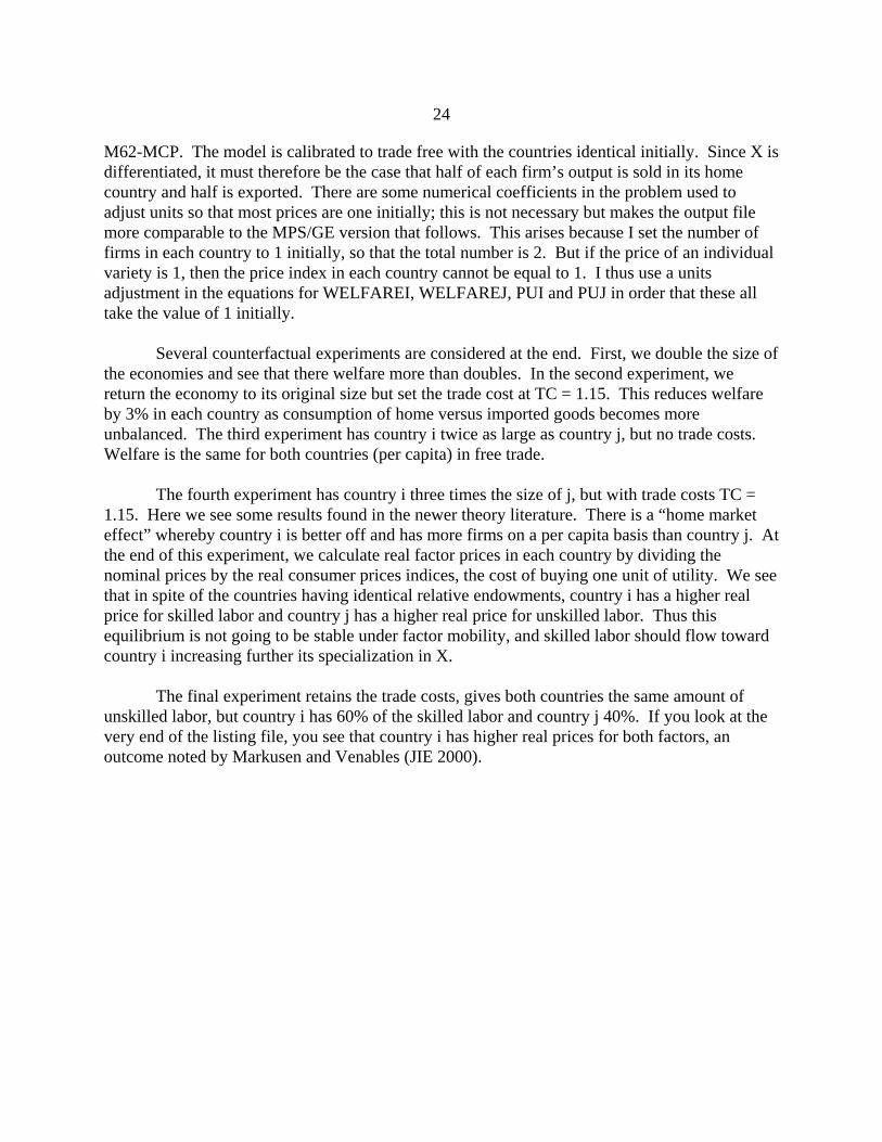
M62-MCP. The model is calibrated to trade free with the countries identical initially. Since X isdifferentiated, it must therefore be the case that half of each firm’s output is sold in its homecountry and half is exported. There are some numerical coefficients in the problem used toadjust units so that most prices are one initially; this is not necessary but makes the output filemore comparable to the MPS/GE version that follows. This arises because I set the number offirms in each country to 1 initially, so that the total number is 2. But if the price of an individualvariety is 1, then the price index in each country cannot be equal to 1. I thus use a unitsadjustment in the equations for WELFAREI, WELFAREJ, PUI and PUJ in order that these alltake the value of 1 initially.

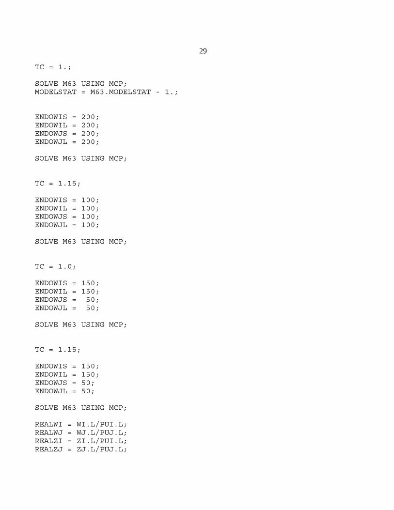
Several counterfactual experiments are considered at the end. First, we double the size ofthe economies and see that there welfare more than doubles. In the second experiment, wereturn the economy to its original size but set the trade cost at TC = 1.15. This reduces welfareby 3% in each country as consumption of home versus imported goods becomes moreunbalanced. The third experiment has country i twice as large as country j, but no trade costs. Welfare is the same for both countries (per capita) in free trade.

The fourth experiment has country i three times the size of j, but with trade costs TC =1.15. Here we see some results found in the newer theory literature. There is a “home marketeffect” whereby country i is better off and has more firms on a per capita basis than country j. Atthe end of this experiment, we calculate real factor prices in each country by dividing thenominal prices by the real consumer prices indices, the cost of buying one unit of utility. We seethat in spite of the countries having identical relative endowments, country i has a higher realprice for skilled labor and country j has a higher real price for unskilled labor. Thus thisequilibrium is not going to be stable under factor mobility, and skilled labor should flow towardcountry i increasing further its specialization in X.

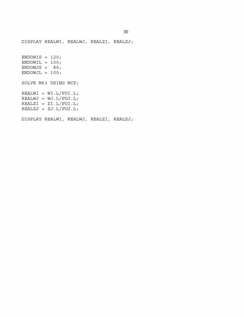
The final experiment retains the trade costs, gives both countries the same amount ofunskilled labor, but country i has 60% of the skilled labor and country j 40%. If you look at thevery end of the listing file, you see that country i has higher real prices for both factors, anoutcome noted by Markusen and Venables (JIE 2000).

25

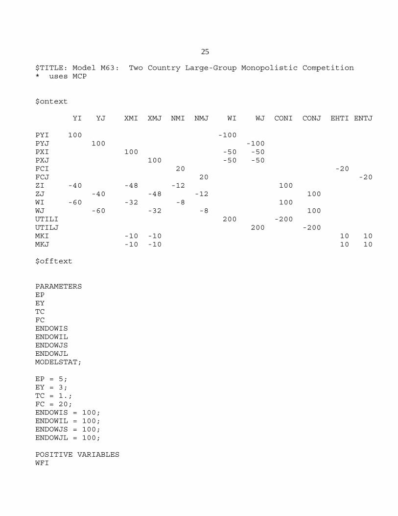
$TITLE: Model M63: Two Country Large-Group Monopolistic Competition* uses MCP

$ontext

YI YJ XMI XMJ NMI NMJ WI WJ CONI CONJ EHTI ENTJ

PYI 100 -100PYJ 100 -100PXI 100 -50 -50PXJ 100 -50 -50FCI 20 -20FCJ 20 -20 ZI -40 -48 -12 100 ZJ -40 -48 -12 100 WI -60 -32 -8 100WJ -60 -32 -8 100UTILI 200 -200UTILJ 200 -200MKI -10 -10 10 10MKJ -10 -10 10 10

$offtext

PARAMETERSEPEYTCFCENDOWISENDOWILENDOWJSENDOWJLMODELSTAT;

EP = 5;EY = 3;TC = 1.;FC = 20;ENDOWIS = 100;ENDOWIL = 100;ENDOWJS = 100;ENDOWJL = 100;

POSITIVE VARIABLESWFI

26

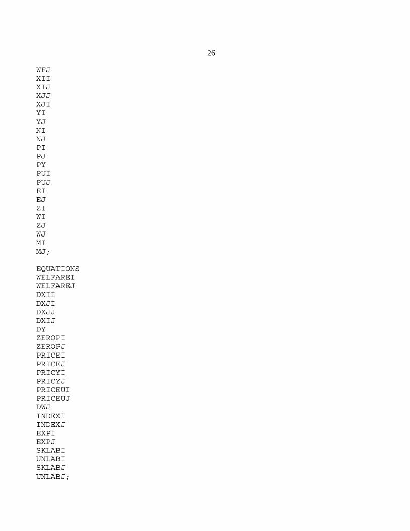
WFJXIIXIJXJJXJIYIYJNINJPIPJPYPUIPUJEI EJZIWIZJWJMIMJ;

EQUATIONSWELFAREIWELFAREJDXIIDXJIDXJJDXIJDYZEROPIZEROPJPRICEIPRICEJPRICYIPRICYJPRICEUIPRICEUJDWJINDEXIINDEXJEXPIEXPJSKLABIUNLABISKLABJUNLABJ;

27

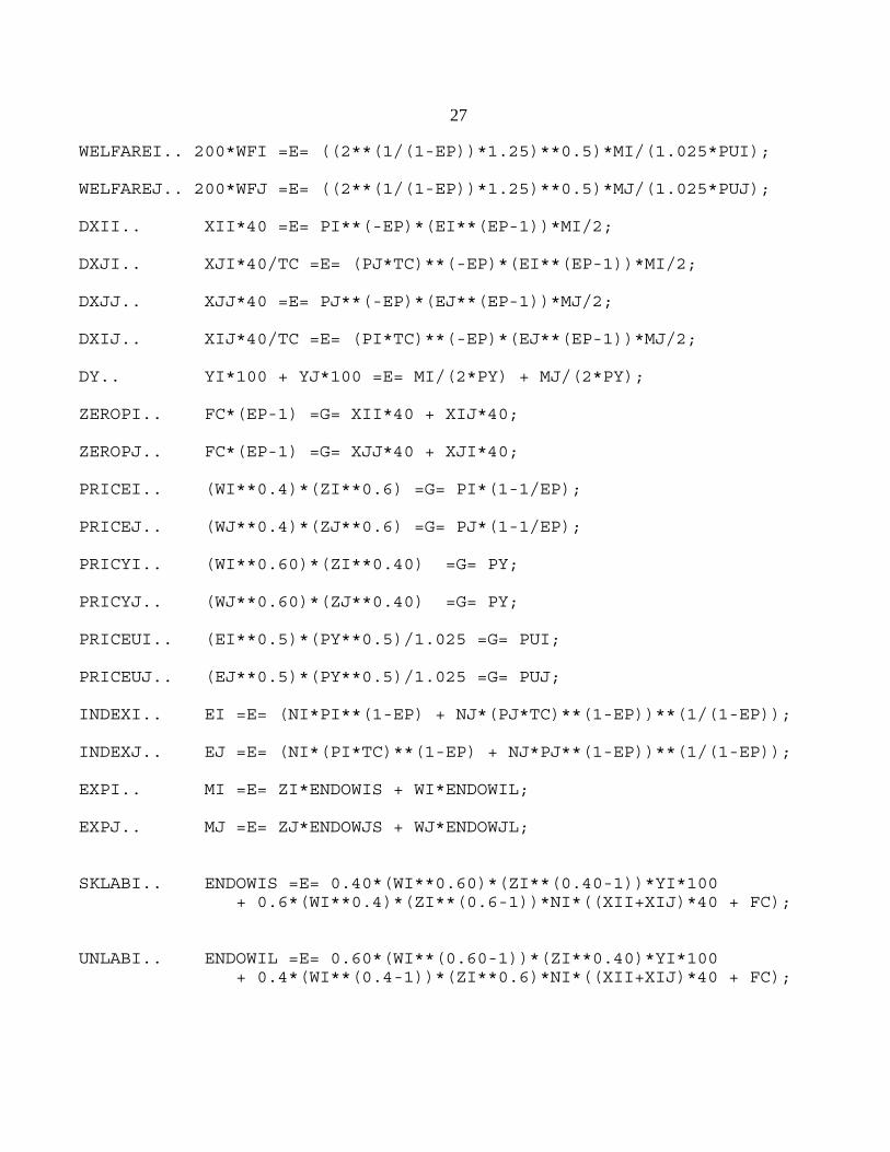
WELFAREI.. 200*WFI =E= ((2**(1/(1-EP))*1.25)**0.5)*MI/(1.025*PUI);

WELFAREJ.. 200*WFJ =E= ((2**(1/(1-EP))*1.25)**0.5)*MJ/(1.025*PUJ);

DXII.. XII*40 =E= PI**(-EP)*(EI**(EP-1))*MI/2;

DXJI.. XJI*40/TC =E= (PJ*TC)**(-EP)*(EI**(EP-1))*MI/2;

DXJJ.. XJJ*40 =E= PJ**(-EP)*(EJ**(EP-1))*MJ/2;

DXIJ.. XIJ*40/TC =E= (PI*TC)**(-EP)*(EJ**(EP-1))*MJ/2;

DY.. YI*100 + YJ*100 =E= MI/(2*PY) + MJ/(2*PY);

ZEROPI.. FC*(EP-1) =G= XII*40 + XIJ*40;

ZEROPJ.. FC*(EP-1) =G= XJJ*40 + XJI*40;

PRICEI.. (WI**0.4)*(ZI**0.6) =G= PI*(1-1/EP);

PRICEJ.. (WJ**0.4)*(ZJ**0.6) =G= PJ*(1-1/EP);

PRICYI.. (WI**0.60)*(ZI**0.40) =G= PY;

PRICYJ.. (WJ**0.60)*(ZJ**0.40) =G= PY;

PRICEUI.. (EI**0.5)*(PY**0.5)/1.025 =G= PUI;

PRICEUJ.. (EJ**0.5)*(PY**0.5)/1.025 =G= PUJ;

INDEXI.. EI =E= (NI*PI**(1-EP) + NJ*(PJ*TC)**(1-EP))**(1/(1-EP));

INDEXJ.. EJ =E= (NI*(PI*TC)**(1-EP) + NJ*PJ**(1-EP))**(1/(1-EP));

EXPI.. MI =E= ZI*ENDOWIS + WI*ENDOWIL;

EXPJ.. MJ =E= ZJ*ENDOWJS + WJ*ENDOWJL;

SKLABI.. ENDOWIS =E= 0.40*(WI**0.60)*(ZI**(0.40-1))*YI*100 + 0.6*(WI**0.4)*(ZI**(0.6-1))*NI*((XII+XIJ)*40 + FC);

UNLABI.. ENDOWIL =E= 0.60*(WI**(0.60-1))*(ZI**0.40)*YI*100 + 0.4*(WI**(0.4-1))*(ZI**0.6)*NI*((XII+XIJ)*40 + FC);

28

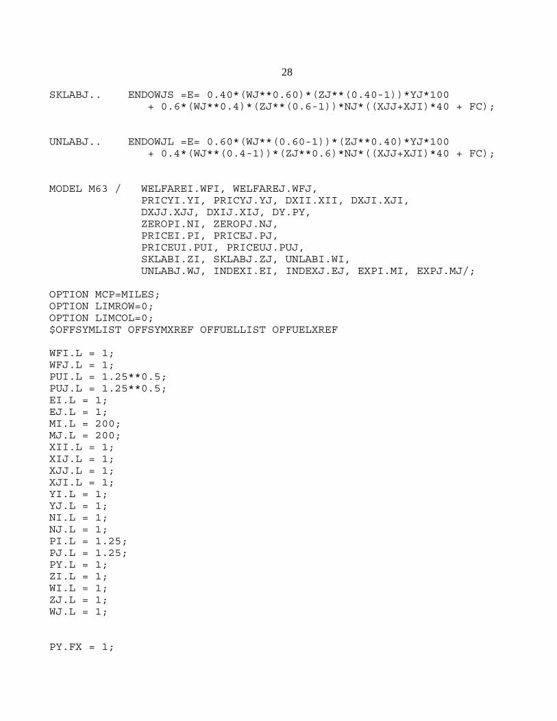
SKLABJ.. ENDOWJS =E= 0.40*(WJ**0.60)*(ZJ**(0.40-1))*YJ*100 + 0.6*(WJ**0.4)*(ZJ**(0.6-1))*NJ*((XJJ+XJI)*40 + FC);

UNLABJ.. ENDOWJL =E= 0.60*(WJ**(0.60-1))*(ZJ**0.40)*YJ*100 + 0.4*(WJ**(0.4-1))*(ZJ**0.6)*NJ*((XJJ+XJI)*40 + FC);

MODEL M63 / WELFAREI.WFI, WELFAREJ.WFJ, PRICYI.YI, PRICYJ.YJ, DXII.XII, DXJI.XJI, DXJJ.XJJ, DXIJ.XIJ, DY.PY, ZEROPI.NI, ZEROPJ.NJ, PRICEI.PI, PRICEJ.PJ, PRICEUI.PUI, PRICEUJ.PUJ, SKLABI.ZI, SKLABJ.ZJ, UNLABI.WI, UNLABJ.WJ, INDEXI.EI, INDEXJ.EJ, EXPI.MI, EXPJ.MJ/;

OPTION MCP=MILES;OPTION LIMROW=0;OPTION LIMCOL=0;$OFFSYMLIST OFFSYMXREF OFFUELLIST OFFUELXREF

WFI.L = 1;WFJ.L = 1;PUI.L = 1.25**0.5;PUJ.L = 1.25**0.5;EI.L = 1; EJ.L = 1;MI.L = 200;MJ.L = 200;XII.L = 1;XIJ.L = 1;XJJ.L = 1;XJI.L = 1;YI.L = 1;YJ.L = 1;NI.L = 1;NJ.L = 1;PI.L = 1.25;PJ.L = 1.25;PY.L = 1;ZI.L = 1;WI.L = 1;ZJ.L = 1;WJ.L = 1;

PY.FX = 1;

29

TC = 1.;


ENDOWIS = 200;ENDOWIL = 200;ENDOWJS = 200;ENDOWJL = 200;


TC = 1.15;



TC = 1.0;



TC = 1.15;



REALWI = WI.L/PUI.L;REALWJ = WJ.L/PUJ.L;REALZI = ZI.L/PUI.L;REALZJ = ZJ.L/PUJ.L;

30

DISPLAY REALWI, REALWJ, REALZI, REALZJ;





31

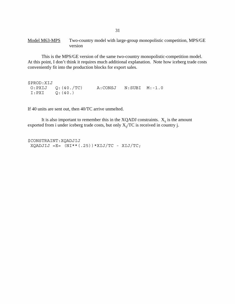
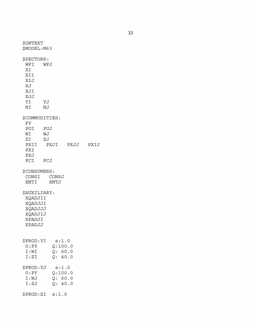
Model M63-MPS Two-country model with large-group monopolistic competition, MPS/GEversion

This is the MPS/GE version of the same two-country monopolistic-competition model. At this point, I don’t think it requires much additional explanation. Note how iceberg trade costsconveniently fit into the production blocks for export sales.

$PROD:XIJ O:PXIJ Q:(40./TC) A:CONSJ N:SUBI M:-1.0 I:PXI Q:(40.)

If 40 units are sent out, then 40/TC arrive unmelted.

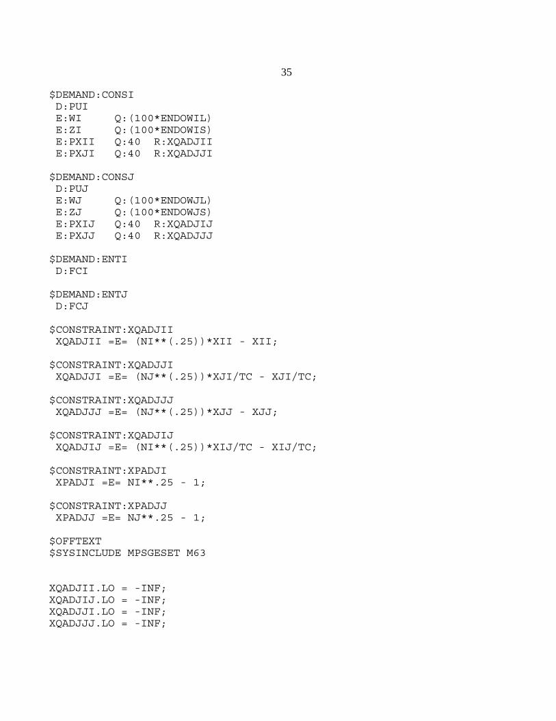
It is also important to remember this in the XQADJ constraints. Xij is the amountexported from i under iceberg trade costs, but only Xij/TC is received in country j.

$CONSTRAINT:XQADJIJ XQADJIJ =E= (NI**(.25))*XIJ/TC - XIJ/TC;

32

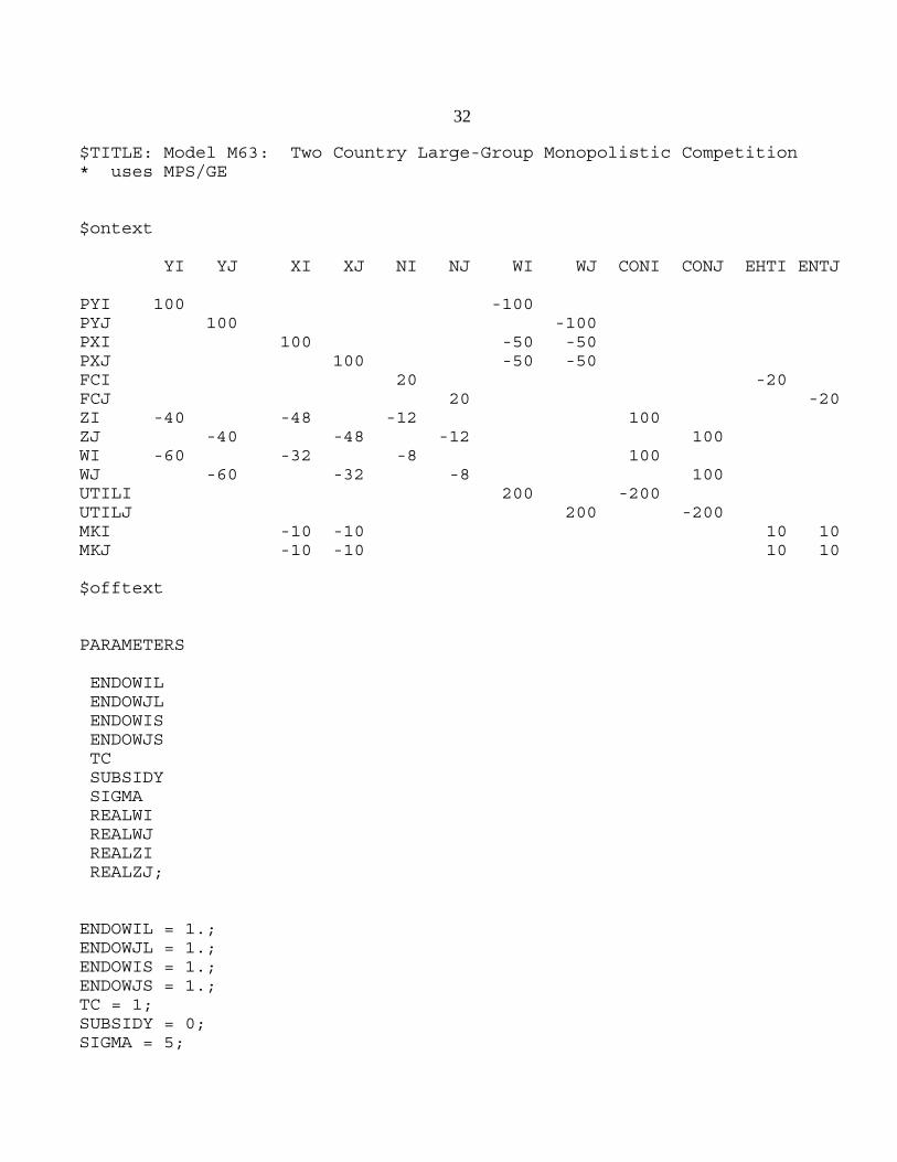
$TITLE: Model M63: Two Country Large-Group Monopolistic Competition* uses MPS/GE

$ontext

YI YJ XI XJ NI NJ WI WJ CONI CONJ EHTI ENTJ

PYI 100 -100PYJ 100 -100PXI 100 -50 -50 PXJ 100 -50 -50FCI 20 -20FCJ 20 -20 ZI -40 -48 -12 100 ZJ -40 -48 -12 100 WI -60 -32 -8 100WJ -60 -32 -8 100UTILI 200 -200UTILJ 200 -200MKI -10 -10 10 10MKJ -10 -10 10 10

$offtext

PARAMETERS ENDOWIL ENDOWJL ENDOWIS ENDOWJS TC SUBSIDY SIGMA REALWI REALWJ REALZI REALZJ;

ENDOWIL = 1.;ENDOWJL = 1.;ENDOWIS = 1.;ENDOWJS = 1.;TC = 1;SUBSIDY = 0;SIGMA = 5;

33

$ONTEXT$MODEL:M63

$SECTORS: WFI WFJ XI XII XIJ XJ XJI XJJ YI YJ NI NJ

$COMMODITIES: PY PUI PUJ WI WJ ZI ZJ PXII PXJI PXJJ PXIJ PXI PXJ FCI FCJ

$CONSUMERS: CONSI CONSJ ENTI ENTJ

$AUXILIARY: XQADJII XQADJJI XQADJJJ XQADJIJ XPADJI XPADJJ

$PROD:YI s:1.0 O:PY Q:100.0 I:WI Q: 60.0 I:ZI Q: 40.0

$PROD:YJ s:1.0 O:PY Q:100.0 I:WJ Q: 60.0 I:ZJ Q: 40.0

$PROD:XI s:1.0

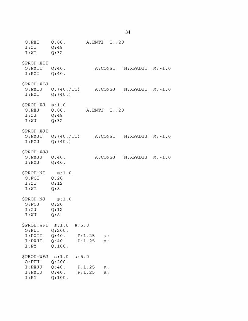
34

O:PXI Q:80. A:ENTI T:.20 I:ZI Q:48 I:WI Q:32

$PROD:XII O:PXII Q:40. A:CONSI N:XPADJI M:-1.0 I:PXI Q:40.

$PROD:XIJ O:PXIJ Q:(40./TC) A:CONSJ N:XPADJI M:-1.0 I:PXI Q:(40.)

$PROD:XJ s:1.0 O:PXJ Q:80. A:ENTJ T:.20 I:ZJ Q:48 I:WJ Q:32

$PROD:XJI O:PXJI Q:(40./TC) A:CONSI N:XPADJJ M:-1.0 I:PXJ Q:(40.)

$PROD:XJJ O:PXJJ Q:40. A:CONSJ N:XPADJJ M:-1.0 I:PXJ Q:40. $PROD:NI s:1.0 O:FCI Q:20 I:ZI Q:12 I:WI Q:8

$PROD:NJ s:1.0 O:FCJ Q:20 I:ZJ Q:12 I:WJ Q:8

$PROD:WFI s:1.0 a:5.0 O:PUI Q:200. I:PXII Q:40. P:1.25 a: I:PXJI Q:40 P:1.25 a: I:PY Q:100.

$PROD:WFJ s:1.0 a:5.0 O:PUJ Q:200. I:PXJJ Q:40. P:1.25 a: I:PXIJ Q:40. P:1.25 a: I:PY Q:100.

35

$DEMAND:CONSI D:PUI E:WI Q:(100*ENDOWIL) E:ZI Q:(100*ENDOWIS) E:PXII Q:40 R:XQADJII E:PXJI Q:40 R:XQADJJI

$DEMAND:CONSJ D:PUJ E:WJ Q:(100*ENDOWJL) E:ZJ Q:(100*ENDOWJS) E:PXIJ Q:40 R:XQADJIJ E:PXJJ Q:40 R:XQADJJJ

$DEMAND:ENTI D:FCI

$DEMAND:ENTJ D:FCJ

$CONSTRAINT:XQADJII XQADJII =E= (NI**(.25))*XII - XII;

$CONSTRAINT:XQADJJI XQADJJI =E= (NJ**(.25))*XJI/TC - XJI/TC;

$CONSTRAINT:XQADJJJ XQADJJJ =E= (NJ**(.25))*XJJ - XJJ;

$CONSTRAINT:XQADJIJ XQADJIJ =E= (NI**(.25))*XIJ/TC - XIJ/TC;

$CONSTRAINT:XPADJI XPADJI =E= NI**.25 - 1;

$CONSTRAINT:XPADJJ XPADJJ =E= NJ**.25 - 1;

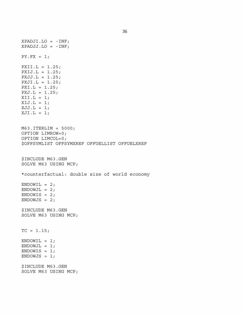
$OFFTEXT$SYSINCLUDE MPSGESET M63

XQADJII.LO = -INF;XQADJIJ.LO = -INF;XQADJJI.LO = -INF;XQADJJJ.LO = -INF;

36

XPADJI.LO = -INF;XPADJJ.LO = -INF;

PY.FX = 1;

PXII.L = 1.25;PXIJ.L = 1.25;PXJJ.L = 1.25;PXJI.L = 1.25;PXI.L = 1.25;PXJ.L = 1.25;XII.L = 1;XIJ.L = 1;XJJ.L = 1;XJI.L = 1;

M63.ITERLIM = 5000;OPTION LIMROW=0;OPTION LIMCOL=0;$OFFSYMLIST OFFSYMXREF OFFUELLIST OFFUELXREF


*counterfactual: double size of world economy

ENDOWIL = 2;ENDOWJL = 2;ENDOWIS = 2;ENDOWJS = 2;


TC = 1.15;

ENDOWIL = 1;ENDOWJL = 1;ENDOWIS = 1;ENDOWJS = 1;


37

TC = 1.0;

ENDOWIL = 1.5;ENDOWJL = .5;ENDOWIS = 1.5;ENDOWJS = .5;


TC = 1.15;

ENDOWIL = 1.5;ENDOWIS = 1.5;ENDOWJL = 0.5;ENDOWJS = 0.5;




ENDOWIL = 1.0;ENDOWIS = 1.2;ENDOWJL = 1.0;ENDOWJS = 0.8;




chapter 6 external economies and monopolistic competition - spot

Documents