1

Chapter 6

Design and Fabrication of High-Q Tuning Inductors for

LF-MF Antennas

6.0 Introduction

The electrically small antennas typical of 630m and 2200m amateur installations can

be represented by the equivalent circuit shown in figure 6.1.

Figure 6.1 - LF-MF antenna equivalent circuit.

The antenna is simply a capacitor in series with a resistor. The capacitive reactance

(Xa) is very large and the series resistance (Ra) is very small. To supply power to the

antenna it's necessary to transform the highly reactive feedpoint impedance of the

antenna to a resistance compatible with the feedline, usually Ri=50Ω. The series

inductor (XL) performs two functions: canceling the input reactance (+XL-Xa=0) and

converting Ra to the desired value for Ri. A tap on the inductor adjusts Ri to the

desired value.

Unfortunately any practical inductor will have losses (represented by RL) which can

reduce the efficiency substantially. The radiation efficiency of the complete antenna

( ) can be expressed by:

(6.1)

2

Where Rr is the radiation resistance, RL is the loss resistance in the inductor, Rg

represents ground system loss, Rc represents conductor loss and miscellaneous other

losses are represented by .... Usually Rr will be very small, a fraction of an ohm, but

RL and Rg are typically much larger. In most cases RL and Rg dominate the efficiency

so every effort must be made to minimize these losses. For an inductor:

(6.2)

(6.3)

Where f is the operating frequency and L is the required inductance.

Minimizing RL to increase Q is the primary tool for maximizing efficiency.

This chapter addresses the design and fabrication of high Q inductors using materials

commonly available at a hardware store. Historically many different coil constructions

have been used but the focus here is on cylindrical single layer air wound coils using

round wire because these are usually the most practical. Examples of flat spiral or

"pancake" inductors, toroidal inductors, non-circular coil forms and basket-weave

windings are briefly mentioned.

The discussion covers a lot of ground at considerable length and it's fair to ask "is all

this verbiage actually useful?" Many articles and even whole books on inductor

design, along with free software design programs, already exist. From a practical point

of view do we really need more?

It turns out that the design of tuning inductors for 630m and 2200m, is significantly

more complicated than a typical HF inductor. LF, MF and HF inductor design must

take into account both skin and proximity effects:

If you measure the resistance of a length of conductor you will discover that

R≈Rdc at low frequencies but as you go up in frequency the resistance increases

substantially. This is called "skin effect".

When a conductor is wound into a coil the current in one turn induces loss in

adjacent turns, this is called "proximity effect".

These two effects complicate the design when high Q is desired but there is another

effect, "self-resonance", which is rarely important at HF but often limits Q at 630m and

2200m:

3

Coil inductors behave very much like transmission lines with a multitude of

harmonically related resonances. The lowest frequency resonance (fr) is often

low enough to significantly impact both inductance and Q.

These three effects must be included in the design of LF-MF inductors but this leads

to complicated calculations. Most amateurs will only occasionally need a new

inductor and a simple, low math method which converges quickly on a good design

is needed. However, some amateurs may want to create optimized designs and are

willing to deal with some complexity. To meet this range of interests the discussion

is divided into two parts:

Part I, "The Basics", begins with graphs allowing one to estimate the required

inductance for a given antenna. To determine the details of the inductor itself,

i.e. number of turns, wire size, coil form diameter, etc, a series of graphs are

provided. The process requires drawing two lines on a single graph and

multiplying a couple of numbers. The rest of part I gives practical examples of

coil fabrication and adjustable inductors along with typical inductor voltages and

currents. This section is intended to provide useful, but not necessarily

optimized, inductors, using a range common materials.

Part II, " Design and Q Optimization", gives explanations for skin effect, proximity

effect and self resonance. Some familiarity with basic algebra is needed to

follow the discussion. The intent of this section is to allow the design of

optimized inductors with the highest practical Q.

4

Part I

The Basics

6.1 How much inductance?

Figure 6.2 -Tuning inductor inductance for resonance at 475 kHz.

When designing a new inductor the very first question is "what value of inductance is

needed?" To resonate the antenna enough inductive reactance (XL) is needed to

cancel the capacitive reactance (Xa) at the feedpoint, i.e. XL=Xa (figure 6.1):

(6.4)

If f is in MHz L will be in μH.

5

To estimate the needed inductance we can convert the values for Xa derived in

chapter 3 to inductance in uH (L) as shown in figures 6.2 and 6.3. In these figures an

italic L identifies the total length in feet of the top-loading wire. It should be pointed out

that although figures 6.2 and 6.3 assume a "T" with a single top-wire, the values for the

loading inductor would be the same for any capacitive top-loading structure which

provides the same amount of capacitive loading. The shape of the hat is not what's

important, it's the shunt capacitance it adds!

The grey box in each figure indicates the range of height (H=20'-60') and top-wire

lengths (L/2=20'-50') seen in typical amateur antennas. From figures 6.2 and 6.3 we

see:

At 475 kHz, for resonance, L varies from 400μH →1000μH.

At 137 kHz, for resonance, L varies from 5mH→12mH.

Figure 6.3 - Tuning inductor inductance for resonance at 137 kHz.

6

6.2 Definitions

Some useful variables can be defined with the help of figure 6.4.

Figure 6.4 - inductor dimensions

c → center-to-center spacing between turns, winding pitch

d → diameter of the winding conductor

D → diameter of the winding

l → coil length

L→ actual inductance at the operating frequency

Lo→ low frequency inductance

lw→ length of the winding conductor

N → number of turns in the winding

Design graphs and equations can be made more general using geometric ratios as

variables. For example:

(d/c) → conductor diameter/turn center-to-center spacing ratio

(l/D) → coil length/diameter ratio

7

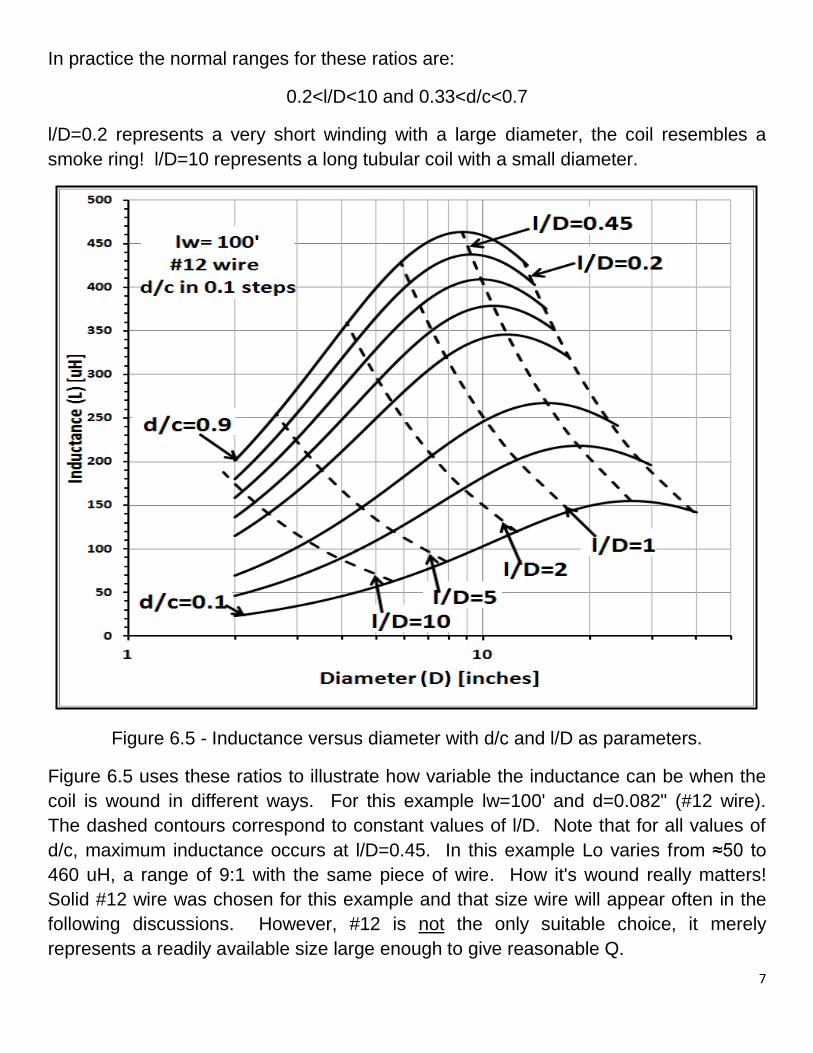
In practice the normal ranges for these ratios are:

0.2<l/D<10 and 0.33<d/c<0.7

l/D=0.2 represents a very short winding with a large diameter, the coil resembles a

smoke ring! l/D=10 represents a long tubular coil with a small diameter.

Figure 6.5 - Inductance versus diameter with d/c and l/D as parameters.

Figure 6.5 uses these ratios to illustrate how variable the inductance can be when the

coil is wound in different ways. For this example lw=100' and d=0.082" (#12 wire).

The dashed contours correspond to constant values of l/D. Note that for all values of

d/c, maximum inductance occurs at l/D=0.45. In this example Lo varies from ≈50 to

460 uH, a range of 9:1 with the same piece of wire. How it's wound really matters!

Solid #12 wire was chosen for this example and that size wire will appear often in the

following discussions. However, #12 is not the only suitable choice, it merely

represents a readily available size large enough to give reasonable Q.

8

6.3 Inductor design using graphs

This section provides a set of graphs from which N, D, lw, etc, can be determined

simply by drawing a pair of straight lines on a graph and then multiplying a couple of

numbers.

Figure 6.6 -Number of turns for a given inductance at 475 kHz.

It is assumed that the desired inductance is known and the problem is to determine N,

D, etc. Several variables must be chosen by the user: coil form diameter D, wire size,

turn spacing ratio d/c and frequency. Figure 6.6 is an example of one of the graphs.

The x-axis is the desired inductance, L. The y-axis shows the number of turns, N,

9

needed for that inductance with a coil form of diameter D, a parameter which the user

has to chose. Each graph is for a specific wire size, frequency and turns spacing ratio

d/c. There is no limit to the possible number of combinations so, as a practical matter,

the graphs are limited to common values:

#14, #12 or #10 wire

d/c=0.33, 0.5 or 0.7

f= 137 kHz or 475 kHz

However, the designer has to chose which combination of variables to use. While the

number of wire sizes available in the graphs is limited they are the most commonly

used in practice for tuning inductors. The graphs for #10 wire will give usefully close

values for #8 wire and the graphs for #14 can be used for #16 with only small error.

The turn-to-turn spacing ratio d/c is an important choice. d/c=0.33 represents a turn-to-

turn spacing (c in figure 6.4) of three wire diameters, which is the same as two wire

diameters between turns. This spacing will usually give the best Q. However, this

large a spacing makes for a larger coil. d/c=0.5, which represents a space of one wire

diameter between each turn, is a compromise. In many cases insulated wire will be

used and may be closely wound on the form. In that case d/c≈0.7 if THHN wire with

PVC insulation is used. Note that the wire diameter d referred to here is the copper

diameter. With insulation the wire diameter will be larger. For example, with #12

THHN wire d≈0.082" but the diameter over the insulation is ≈0.117"-0.120". Close

winding this wire results in c≈0.240" and d/c≈0.7. Other wire sizes give similar d/c

ratios.

Looking through the graph sets you will see the range of values for D is not the same

everywhere, some graphs show D=4"-20" while others are cut off at D=14". Some of

the contours, for a given D, are abbreviated. This is the result of two limitations: the

length diameter ratio l/D and the minimum allowable self-resonant frequency fr. When

deriving the graphs in the spreadsheet, l/D is limited to 0.2-10. The effect of self-

resonance is explained in Part II. These graphs are also limited by the minimum

allowable self-resonant frequency fr. the minimums are fr>340 kHz for 2200m and

>1.2 MHz for 630m. Contours corresponding to design solutions which fall outside the

range of these limitations have been omitted.

The graphs are divided into two groups, one for 630m (section 6.3.1) and the other for

2200m (section 6.3.2).

10

Figure 6.7 - Inductance versus number of turns.

Reasons for this division can be illustrated with figures 6.7 and 6.8. By way of an

example, let's assume a 10" diameter (D) coil form, a 5 gallon bucket perhaps, and

some #12 wire. Figure 6.7 shows the value of L at three frequencies, 10, 137 and 475

kHz, as a function of the number of turns (N). At 10 kHz L varies almost linearly with N

but as the frequency is increased the relationship between L and N changes. At 137

kHz there is a marked increase in L for N>200 turns but the increase is much more

dramatic at 475 kHz where the change starts at <80 turns. What we're seeing is the

effect of self-resonance. This effect might appear to be a plus since you need less

wire (lw) for a given L but that's deceptive as shown in the next figure.

11

Figure 6.8 - Q versus number of turns.

Figure 6.8 is a graph of inductor Q at 137 and 475 kHz as a function of N. This graph

includes skin, proximity and self-resonance effects. As turns are added L increases

and so does Q but at some point Q peaks and then falls rapidly. For reasons

explained in Part II, only the region below the peak value of Q is useful. In this

particular example we have to limit N<100 at 475 kHz and 250 at 137 kHz. Referring

back to figure 6.7, this limits L<1200 uH at 475 kHz and <3.5 mH at 137 kHz.

12

6.3.1 Design

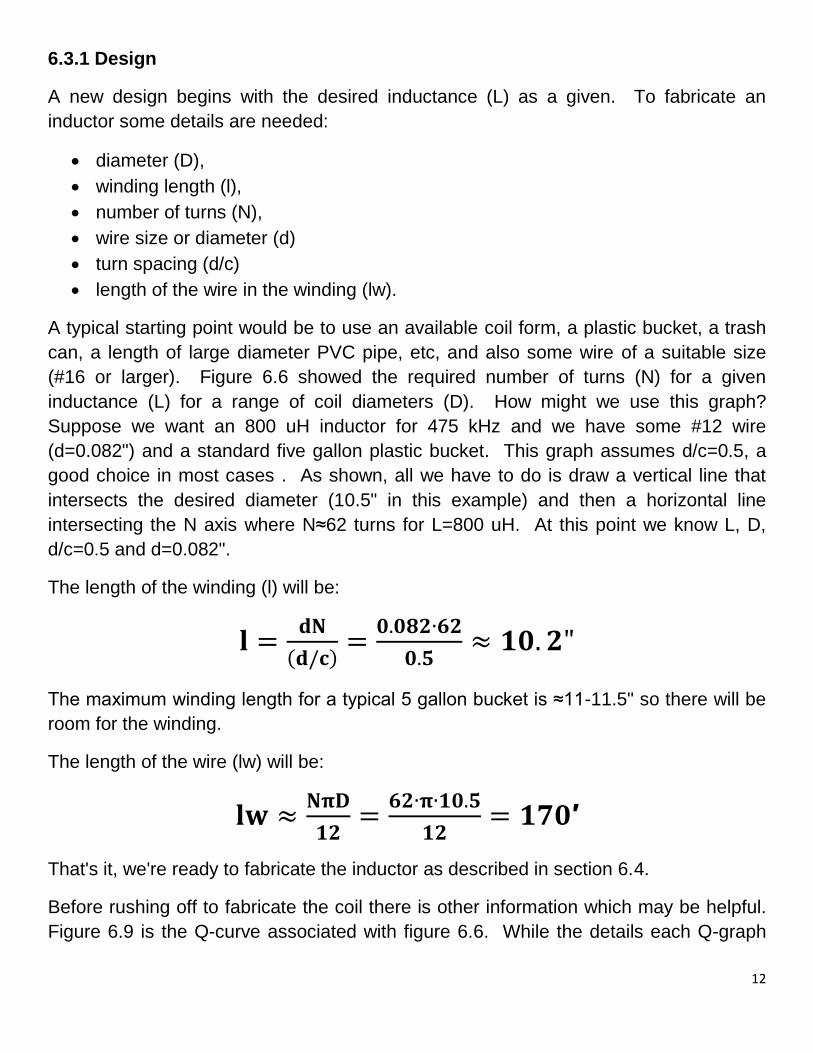
A new design begins with the desired inductance (L) as a given. To fabricate an

inductor some details are needed:

diameter (D),

winding length (l),

number of turns (N),

wire size or diameter (d)

turn spacing (d/c)

length of the wire in the winding (lw).

A typical starting point would be to use an available coil form, a plastic bucket, a trash

can, a length of large diameter PVC pipe, etc, and also some wire of a suitable size

(#16 or larger). Figure 6.6 showed the required number of turns (N) for a given

inductance (L) for a range of coil diameters (D). How might we use this graph?

Suppose we want an 800 uH inductor for 475 kHz and we have some #12 wire

(d=0.082") and a standard five gallon plastic bucket. This graph assumes d/c=0.5, a

good choice in most cases . As shown, all we have to do is draw a vertical line that

intersects the desired diameter (10.5" in this example) and then a horizontal line

intersecting the N axis where N≈62 turns for L=800 uH. At this point we know L, D,

d/c=0.5 and d=0.082".

The length of the winding (l) will be:

The maximum winding length for a typical 5 gallon bucket is ≈11-11.5" so there will be

room for the winding.

The length of the wire (lw) will be:

That's it, we're ready to fabricate the inductor as described in section 6.4.

Before rushing off to fabricate the coil there is other information which may be helpful.

Figure 6.9 is the Q-curve associated with figure 6.6. While the details each Q-graph

13

will depend on specific values for wire size, d/c and frequency, we can make some

general observations helpful for future designs.

Figure 6.9 - Q

This example has Q≈685 which is very respectable considering the inexpensive

materials. We see that increasing D would improve Q a bit more but there is a limit.

By the time D=14", Q is approaching it's maximum value for this particular set of

variables. Up to a point larger D gives higher Q. The Q-graph also illustrates the

effect smaller diameter coil forms. For D=8" the Q is still quite good but further

reductions in diameter sharply decrease Q and Q is now on the falling side of

maximum. As a general rule LF-MF tuning inductors should have a diameter of 8" or

more for reasonable Q. This becomes more acute as the value of L increases.

Now let's change the example to assume we want a 2 mH inductor for 2200m wound

on the same bucket. The appropriate graph for 137 kHz is shown in figure 6.10.

14

Figure 6.10 - Number of turns for a given inductance.

15

Figure 6.11 - Q

N≈145 turns so the length of the winding (l) will be:

This is too long for the space available on the bucket (≈11 inches)! A longer form will

be needed. The fabrication of coil forms of arbitrary size using inexpensive PVC pipe

is shown in section 6.5 and we could use one of those instead. Figure 6.11 shows the

Q-graph associated with figure 6.10. With D=10.5" Q≈493 which is respectable but the

16

Q-graph also shows that if the diameter is increased to 20", Q≈570, a substantial

improvement. Returning to figure 6.10, N is now ≈60 turns. The length of the winding

(l) will be:

The length of the wire in the winding (lw) for D=20" will be:

By using a larger diameter we have increased Q and reduced the amount of wire but

this requires the fabrication of a coil form.

A special coil form is not the only possibility. If we want to use the five gallon bucket

we could reduce the wire size and the spacing: for example use #14 wire (d=0.064")

and d/c≈0.7. d/c≈0.7 is what you would expect to get when THHN insulated house

wire, close wound, is used. Figure 6.12 is the appropriate graph. For L=2 mH and

D=10.5", N≈95 turns. From this l≈8.7" which will fit on the bucket and lw≈261'. The

price for going to this design is lower Q: Q≈tbd.

This is a simple process:

choose the wire size and d/c ratio

select an appropriate graph,

draw a vertical to intersect the desired diameter D contour

draw a horizontal line from that intersection to the y-axis

perform two simple multiplications.

The downside is the need for a larger number of graphs to cover the wide range of

possible wire sizes and spacing ratios. Even with the substantial number of graphs

given, only a small range of possibilities are addressed directly. If this simple approach

is not sufficient the information in Part II can be used to design a well optimized

inductor for a specific application but that requires the use of some math.

17

Figure 6.12 -N versus L.

18

6.3.2 475 kHz design graphs

Figure 6.13 - N versus L.

19

Figure 6.14 - N versus L.

20

Figure 6.15 - N versus L.

21

Figure 6.16 - N versus L.

22

Figure 6.17 - N versus L.

23

Figure 6.18 - N versus L.

24

Figure 6.19 - N versus L.

25

Figure 6.20 - N versus L.

26

Figure 6.21 - N versus L.

27

6.3.3 137 kHz design graphs

Figure 6.22 - N versus L.

28

Figure 6.23 - N versus L.

29

Figure 6.24 - N versus L.

30

Figure 6.25 - N versus L.

31

Figure 6.26 - N versus L.

32

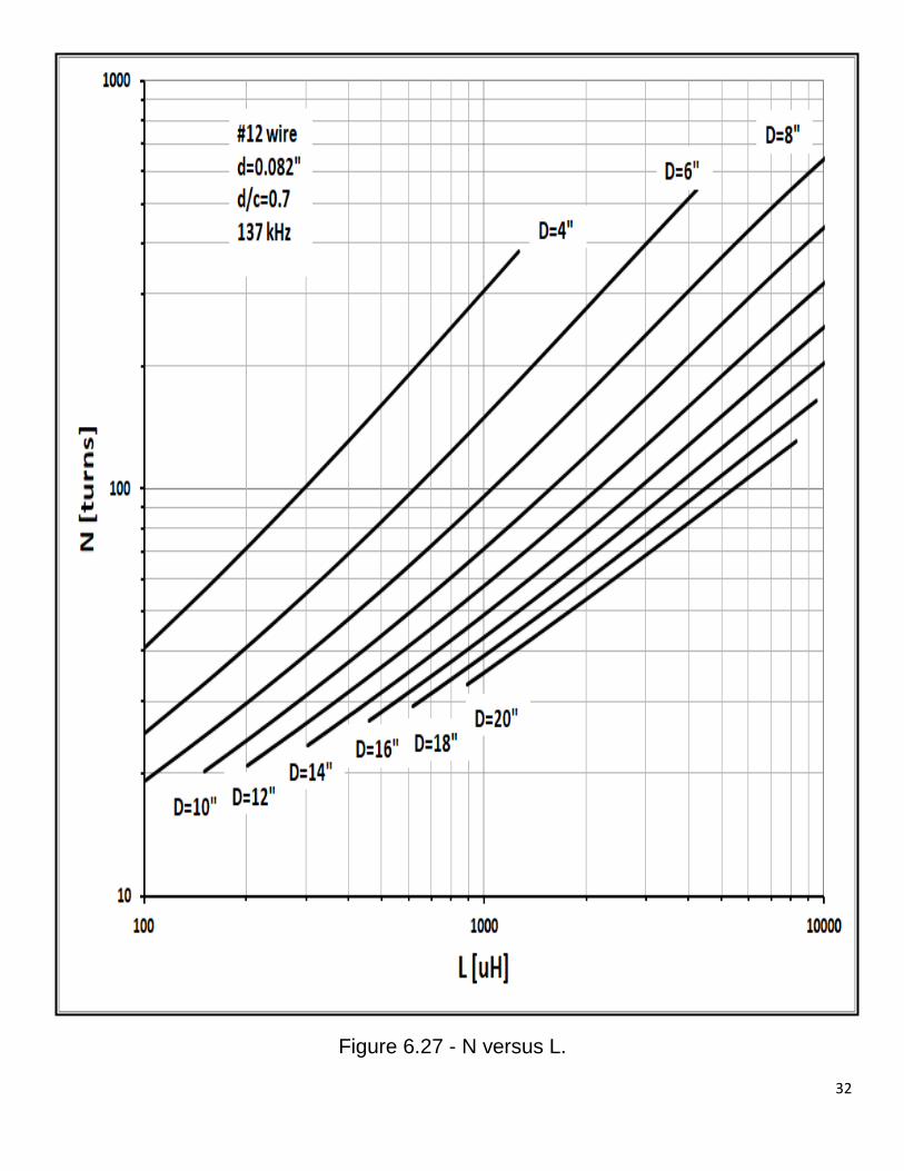
Figure 6.27 - N versus L.

33

Figure 6.28 - N versus L.

34

Figure 6.29 - N versus L.

35

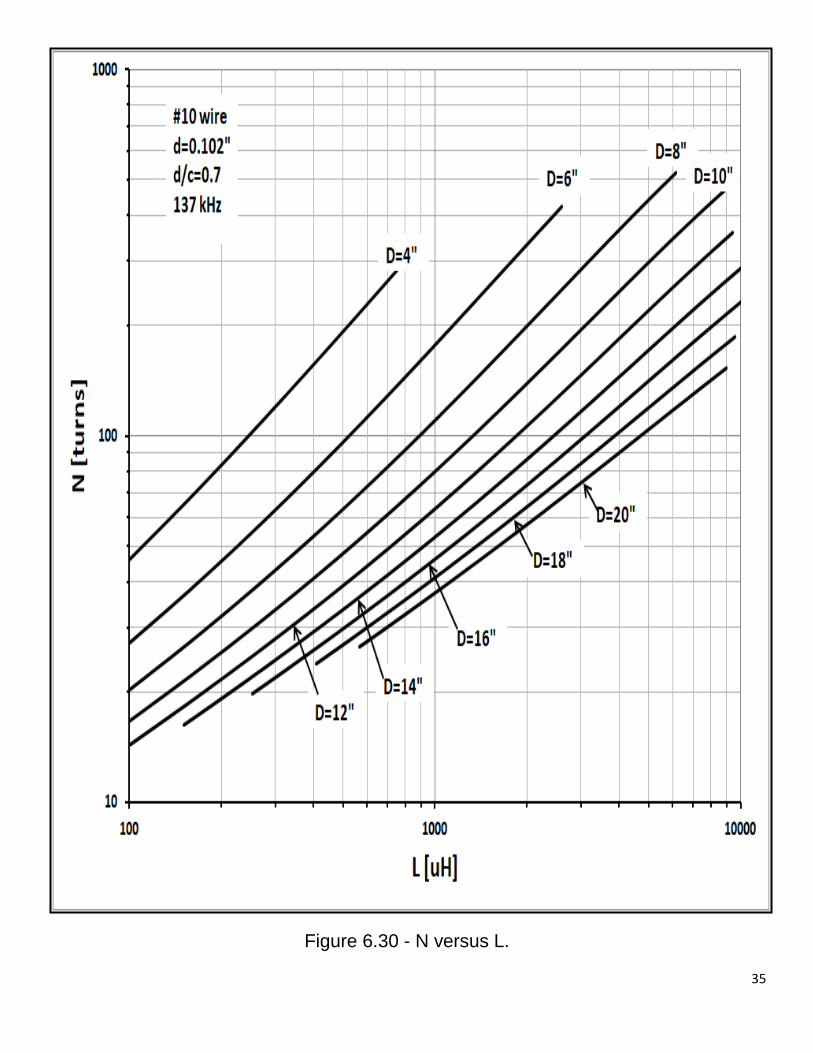
Figure 6.30 - N versus L.

36

6.4 Bucket inductors

As shown in figure 6.31 a plastic bucket can be used as a coil form. Often insulated

THHN wire is used for the winding. Because it's widely used in home wiring this wire is

relatively inexpensive and widely available but some thought must be given to the

winding process. Because the bucket is smooth plastic with some taper and the wire

insulation is also smooth plastic, as illustrated in figure 6.32, the wire tends to move

around as the coil is moved. There is a simple trick which helps: attach several (6-8)

vertical strips of double sided mounting tape vertically before winding. This does a

good job of holding the wire in place

Figure 6.31 - Plastic bucket inductor examples.

Figure 6.32 shows 1/2" pipe attached to the top and bottom of the bucket using

hardware store stanchions. There are square plywood blocks on the inner sides of the

bucket bottom and lid to stiffen them. The stanchions are attached with screws

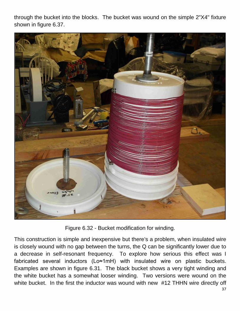
37

through the bucket into the blocks. The bucket was wound on the simple 2"X4" fixture

shown in figure 6.37.

Figure 6.32 - Bucket modification for winding.

This construction is simple and inexpensive but there's a problem, when insulated wire

is closely wound with no gap between the turns, the Q can be significantly lower due to

a decrease in self-resonant frequency. To explore how serious this effect was I

fabricated several inductors (Lo≈1mH) with insulated wire on plastic buckets.

Examples are shown in figure 6.31. The black bucket shows a very tight winding and

the white bucket has a somewhat looser winding. Two versions were wound on the

white bucket. In the first the inductor was wound with new #12 THHN wire directly off

38

the original spool so it was smooth allowing a very tight winding with the same length

as shown on the black bucket. After completing some measurements the wire was

unwound and used for other experiments. As a result the wire became a bit lumpy. I

then rewound this wire on the same bucket but this time the winding was significantly

longer, ≈+1" and looser with small air gaps between the turns.

Figure 6.33 - Comparison between tight and loose windings.

39

Figure 6.33 compares the Q measurements with tight and loose windings compared against calculated values. There is a substantial difference! As shown in figure 6.34, in a tight winding the insulation on each turn is pressed closely to the turns on either side which increases the winding capacitance and reduces the self-resonant frequency which in turn reduces the Q.

Figure 6.34 - Cross section of an insulated wire winding.

It should be noted that the reduction in Q with an insulated wire winding is due to a lower self-resonant frequency (fr) not dielectric loss in the insulation. Section 6.12 has an explanation of this. At MF and below PVC insulation and high density polyethelene (HDPE) buckets appear to have very little dielectric loss. Not all buckets are HDPE, while the HDPE is common there are many lower quality buckets on the market. Look on the bottom of a prospective bucket, there should be a small triangle with 2 in it and HDPE underneath. The wall thickness of the bucket in mils should also be there. Food quality buckets are usually 90 mils and common hardware store buckets, 70 mils. If you see no markings be a bit wary. The bucket may be just fine but you can't tell.

Summarizing, bucket inductors can be very good with Q>400 or even >600 but you have to be a bit careful with the windings. You also need to calculate fr to be sure you're not pushing your luck.

40

6.5 Frame or Cage coil forms

Figure 6.35 - PVC cage coil form.

PVC pipe combined with standard fittings provides an inexpensive and flexible way to

construct a coil form of arbitrary size as the example in figure 6.35 shows. In this

example the octagonal rings are 1/2" pipe joined with 45° elbows. Because the

winding compresses the form it's not necessary to glue the rings making it much easier

to fabricate and adjust! The eight vertical supports used 3/4" pipe with slots cut at

intervals (=c) to hold the wire. Figure 6.36 shows a practical way to cut slots.

Attaching the supports to a board makes it much easier to align all the slots and

mounting holes.

41

Figure 6.36 - Cutting the wire slots.

Figure 6.37 - Winding the inductor.

42

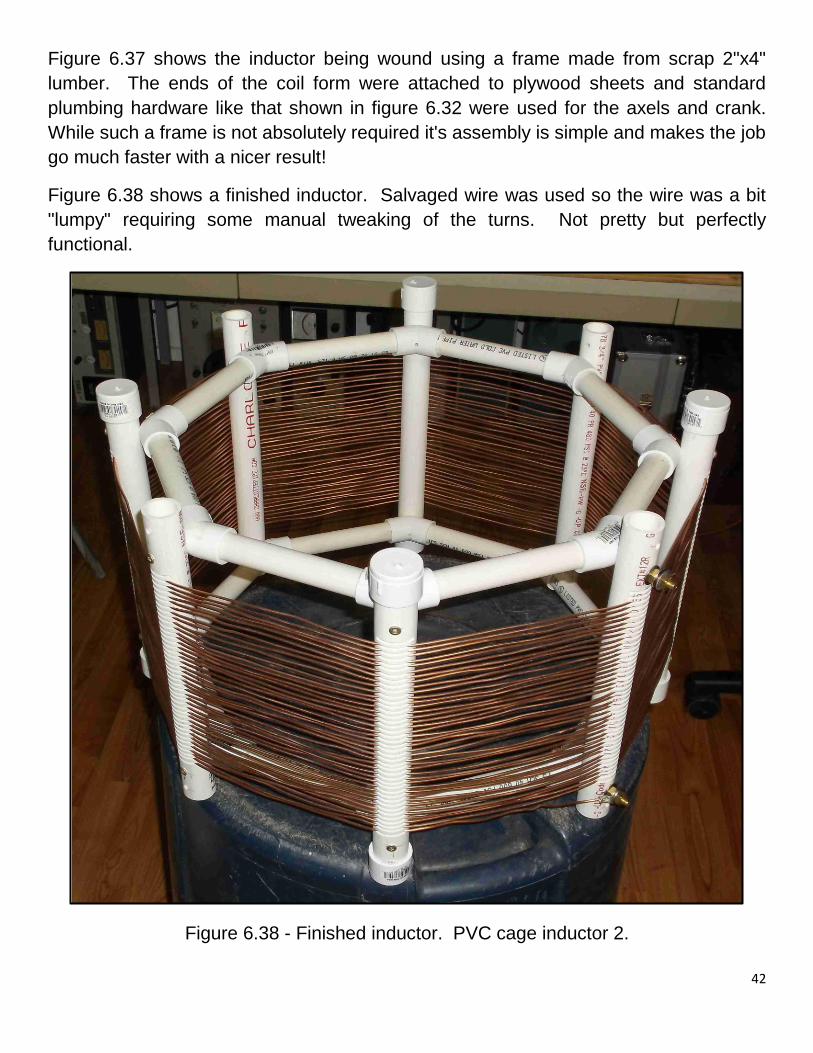
Figure 6.37 shows the inductor being wound using a frame made from scrap 2"x4"

lumber. The ends of the coil form were attached to plywood sheets and standard

plumbing hardware like that shown in figure 6.32 were used for the axels and crank.

While such a frame is not absolutely required it's assembly is simple and makes the job

go much faster with a nicer result!

Figure 6.38 shows a finished inductor. Salvaged wire was used so the wire was a bit

"lumpy" requiring some manual tweaking of the turns. Not pretty but perfectly

functional.

Figure 6.38 - Finished inductor. PVC cage inductor 2.

43

The measured Q for this inductor is shown in figure 6.39. At 137 kHz QL≈435 and at

475 kHz Q ≈680!

Figure 6.39 - Example inductor measured QL.

A clever example of a very light weight inductor (≈18"X18") is shown in figure 6.40.

Pat, W5THT, fabricated the coil form by wrapping F/G mat around a cardboard tube.

He then impregnated the mat with epoxy and when it had cured, soaked the assembly

in water to soften the cardboard for removal, leaving a thin shell on which he wound

1/2" wide copper tape. A protective covering of paint was then applied. The light

weight of the inductor allowed him to hoist it to the top of his vertical where it joined the

capacitive hat.

44

Figure 6.40 - Pat W5THT, foil wound lightweight inductor.

For 600m and 2200m a foil thickness of 0.005"→0.010" would be close to optimum.

One could also purchase a sheet of thin plastic and roll it to make the coil form.

45

6.6 Variable inductors

In most cases the loading inductor will need to be adjustable, at least to some degree,

and there are a number of possibilities:

1) Make the inductance larger than needed and prune the coil.

2) Make the inductance larger than needed and place taps on the winding.

3) Use two inductors in series, one with a fixed value for the bulk of the inductance and

the other a smaller variable inductor large enough for the needed tuning range.

Option 1 is very simple but it's a one shot deal. In most cases the antenna will require

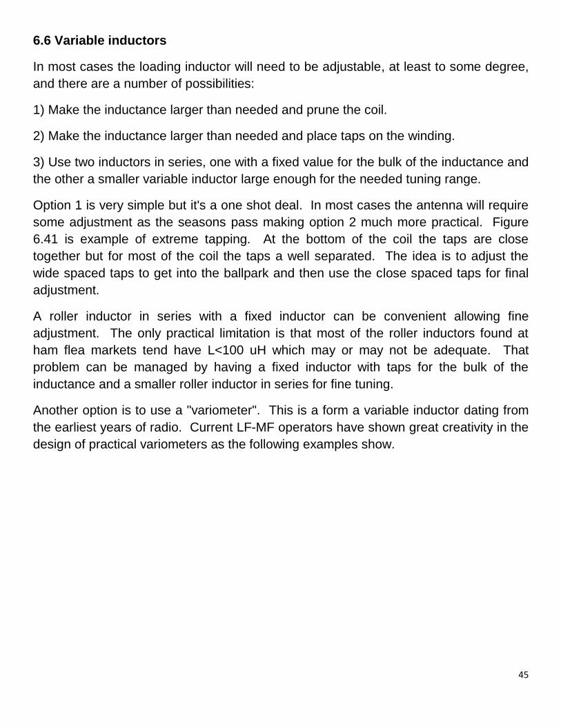
some adjustment as the seasons pass making option 2 much more practical. Figure

6.41 is example of extreme tapping. At the bottom of the coil the taps are close

together but for most of the coil the taps a well separated. The idea is to adjust the

wide spaced taps to get into the ballpark and then use the close spaced taps for final

adjustment.

A roller inductor in series with a fixed inductor can be convenient allowing fine

adjustment. The only practical limitation is that most of the roller inductors found at

ham flea markets tend have L<100 uH which may or may not be adequate. That

problem can be managed by having a fixed inductor with taps for the bulk of the

inductance and a smaller roller inductor in series for fine tuning.

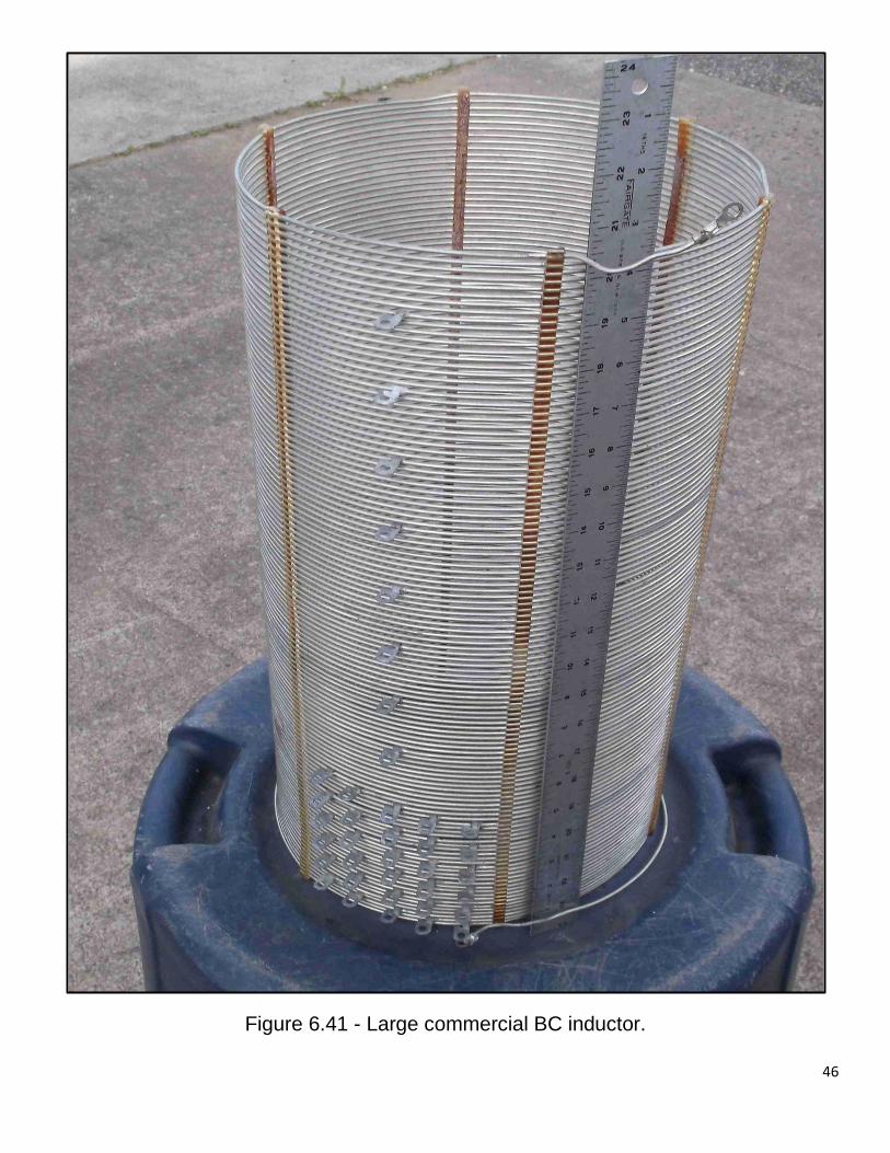
Another option is to use a "variometer". This is a form a variable inductor dating from

the earliest years of radio. Current LF-MF operators have shown great creativity in the

design of practical variometers as the following examples show.

46

Figure 6.41 - Large commercial BC inductor.

47

Figure 6.42- KB5NJD variometer.

Figures 6.42 and 6.43 are examples fabricated by John, KB5NJD. The base inductor

is wound on the outside of a plastic bucket. Inside the bucket is a smaller rotatable

inductor. The two inductors are connected in series. By rotating the inner inductor the

total inductance goes from the sum of both to the difference. Usually a variation of

10% is possible. Given the need for adjustment at inconvenient times (pitch dark and

snowing) many variometers have some form of remote tuning. As figures 6.43-6.52

show there's no shortage of innovation. KB5NJD used an inexpensive TV antenna

rotor! Some of these examples are almost works of art.

48

Figure 6.43 - John, KB5NJD variometer adjustment with a TV rotor.

Figure 6.44 - Jay, W1VD, WD2XNS variometer.

49

Figure 6.45 - Jay, W1VD, WD2XNS variometer.

Figure 6.46 - Jay, W1VD, WD2XNS variometer enclosure.

50

Figure 6.47 - Steve, KK7UV, variometer.

Figure 6.48- Paul, WA2XRM, variometer enclosure w/remote drive.

51

Figure 6.49 - Laurence, KL7L, variometer drive.

Figure 6.50 - Laurence, KL7L, variometer enclosure.

52

Figure 6.51 -Neil, W0YSE, variometer.

Figure 6.52 - W0YSE tuning unit circuit diagram.

53

Figure 6.53 - W0YSE variometer location.

Neil, W0YSE, has located his variometer just outside a window of the shack.

Adjustment is manual: open window, twist knob, close window.

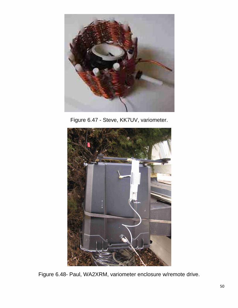
As shown in figures 6.54 and 6.55, Ralph, W5JGV, has built lovely variometers using

PVC pipe. The inductance of these variometers is not large but they work fine for fine

adjustment in combination with a tapped main inductor.

54

Figure 6.54 -Ralph, W5JGV variometer.

Figure 6.55 - Ralph, W5JGV variometer

55

6.7 Winding voltages, currents and power dissipation

The current at the base of the antenna (Io) is also the current in the inductor. The

voltage across the inductor is the same as the voltage at the base of the antenna (Vo).

Io is determined by the radiated power Pr and the radiation resistance Rr:

(6.5)

As explained in chapter 1, the maximum radiated power (Pr) is limited to 1.67W on

630m and 0.33W on 2200m. Combining the band specific values for Pr with Rr values

we can use equation (6.21) to create the graphs for Io shown in figures 6.56 and 6.57.

Note that L is the overall length of the top-wire in feet in all of the graphs in this section.

Vo is the voltage at the feedpoint:

(6.6)

We can use typical Xi values from chapter 3 to generate values for Vo as shown in

figures 6.58 and 6.59. Despite the low radiated powers (Pr) the voltages at the base

will often be >1kV and can be much higher, particularly when H is small. This must be

kept in mind when selecting a base insulator. A high Vo also means there will be

significant voltage turn-to-turn in the loading inductor and across matching network

components.

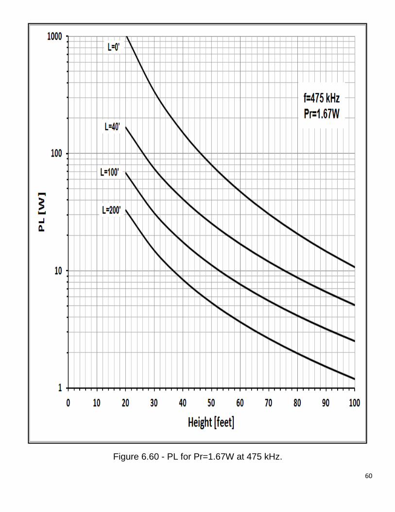
PL is the power dissipated in the loading inductor, PL=Io2RL. As shown in figures 6.60

and 6.61 this power can easily be >100W (assuming that level of transmitter power is

available). The loading inductor must dissipate PL without damage! In general the

larger the physical size of the inductor the better heat can be dissipated. QL=300 is

assumed for both 137 kHz and 475 kHz. This is a bit pessimistic given the earlier

discussion since increasing QL reduces PL proportionately:

(6.7)

In short verticals with limited top-loading Io, Vo and PL can be very high. The key to

reducing these values is to use sufficient top-loading.

56

Figure 6.56 - Io for Pr=1.67W at 475 kHz.

57

Figure 6.57 - Io for Pr=0.33W at 137 kHz.

58

Figure 6.58 - Vo for Pr=1.67W at 475 kHz.

59

Figure 6.59 - Vo for Pr=0.33W at 137 kHz.

60

Figure 6.60 - PL for Pr=1.67W at 475 kHz.

61

Figure 6.61 - PL for Pr=0.33W at 137 kHz.

62

6.8 Enclosures

Most amateurs will use some form of large plastic box for the tuning inductor

enclosure. These are inexpensive, readily available in a very wide range of sizes and

have little or no effect on QL. One shortcoming of typical plastic containers is their

susceptibility to degradation from the UV in sunlight. A simple coat of white house

paint is usually enough to allow them to last several years. Metal enclosures can also

be used although large enclosures will usually be custom fabricated. In general a

metal enclosure needs to be substantially larger than the inductor. In particular the

spacing from the ends of the coil to the enclosure wall should be at least equal to the

coil diameter. A conducting enclosure will tend to reduce both L and QL if it isn't large

enough.

6.9 Coupling, isolation and matching

When using a counterpoise the antenna feed has to be decoupled (isolated) from

ground but still provide a ground referenced 50Ω feedpoint for the transmitter. The

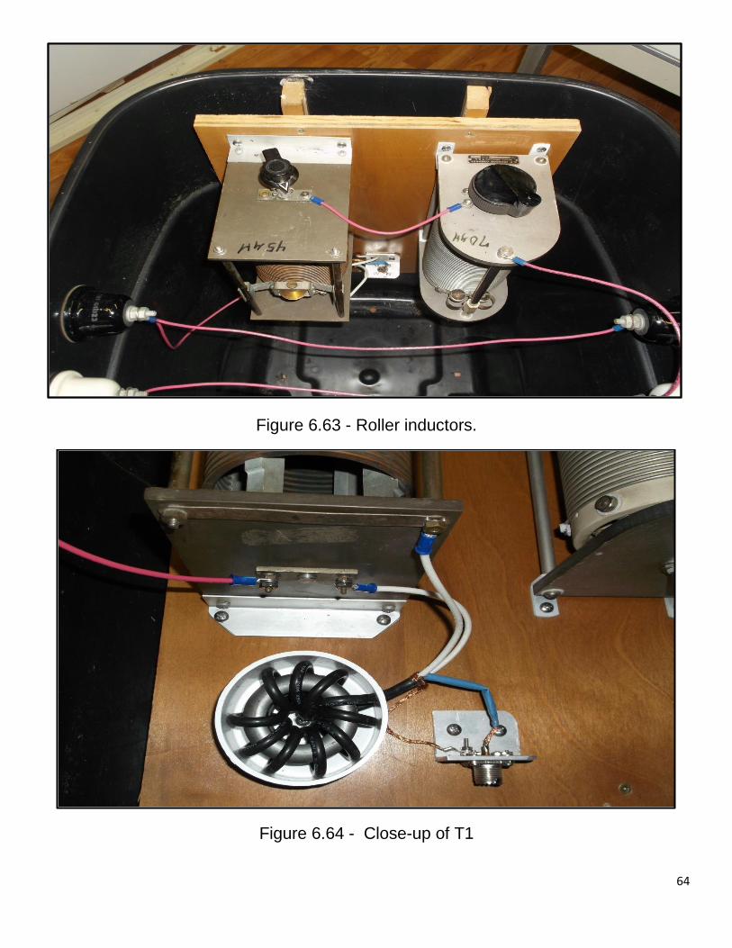
scheme I used is shown in figure 6.62. My inductor (L) is actually two roller inductors

in series but one could also use a single inductor with taps to accomplish the same

end. One inductor is adjusted to resonate the antenna and the other is adjusted to

provide 50Ω across the "tap". HV isolation is provided by T1 which has ten turns of

RG8X wound on a stacked pair of 2.4" FairRite type 77 material ferrite cores (Mouser

P/N 623-5977003801). The physical arrangement is shown in figures 6.63 and 6.64.

T1 has a 1:1 turns ratio. The center conductor forms the secondary winding which is

connected to the antenna. The shield forms the primary winding which is connected to

the UHF jack and then connected to the feedline back to the transmitter. From the

coax used for winding there is ≈50pF of primary-secondary capacitance (≈6700Ω @

475 kHz). The purpose of the choke shown in figure 6.62 is to isolate this parasitic

capacitance. However, I ran out of suitable cores so the choke is not present in figure

6.64. The cores are on order!

63

Figure 6.62 - N6LF matching-isolation scheme.

64

Figure 6.63 - Roller inductors.

Figure 6.64 - Close-up of T1

65

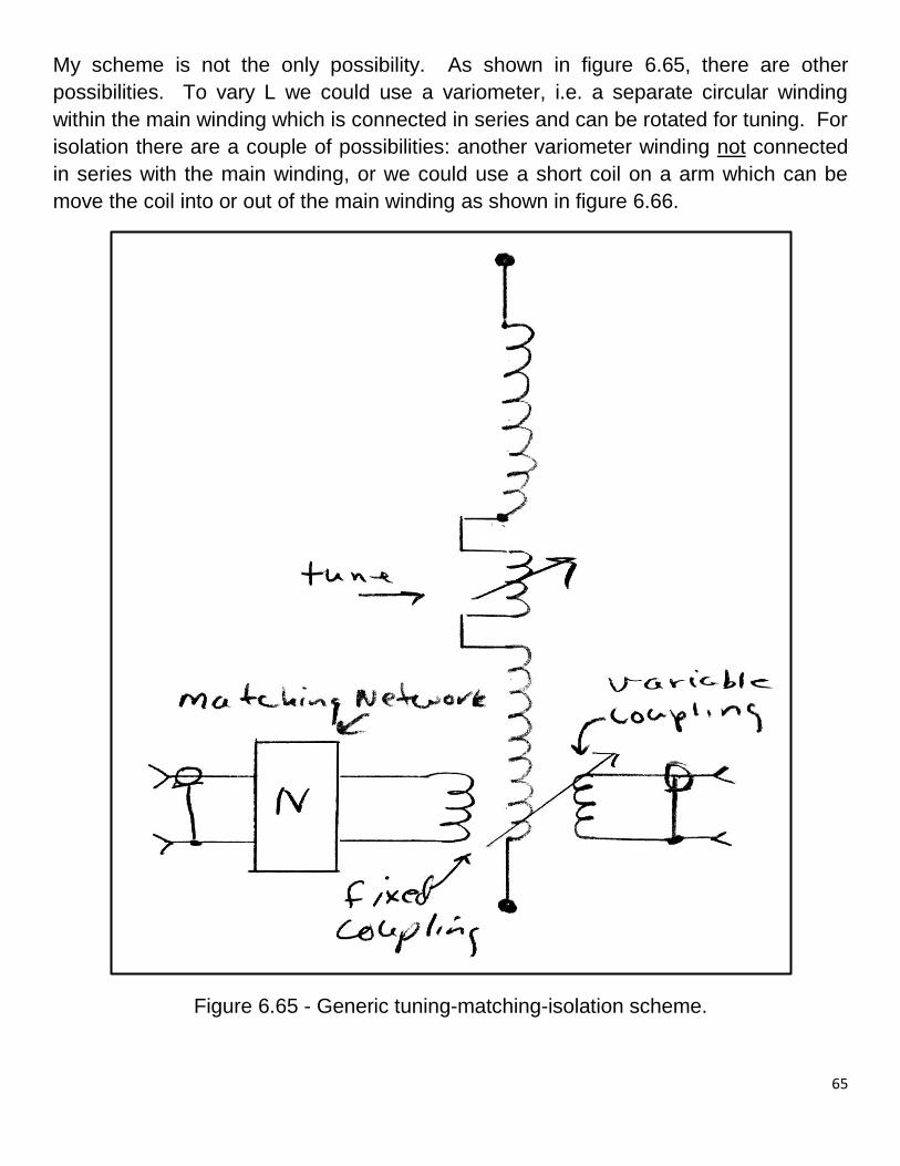
My scheme is not the only possibility. As shown in figure 6.65, there are other

possibilities. To vary L we could use a variometer, i.e. a separate circular winding

within the main winding which is connected in series and can be rotated for tuning. For

isolation there are a couple of possibilities: another variometer winding not connected

in series with the main winding, or we could use a short coil on a arm which can be

move the coil into or out of the main winding as shown in figure 6.66.

Figure 6.65 - Generic tuning-matching-isolation scheme.

66

Figure 6.66 - Swinging link coupling example.

Figure 6.66 was taken from the 1949 edition of the ARRL Radio Amateur's Handbook.

It shows an example of "swinging link" coupling where the coupling link (a small coil) is

attached to an arm which rotates the link into and out of the winding.

67

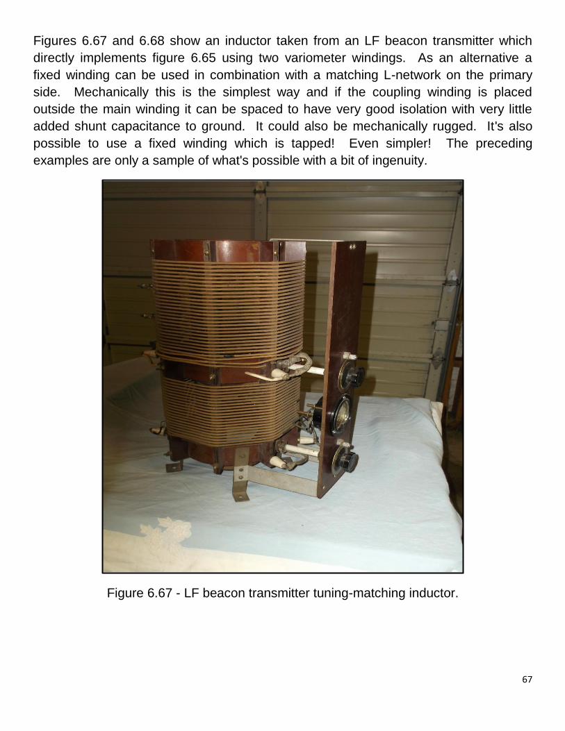
Figures 6.67 and 6.68 show an inductor taken from an LF beacon transmitter which

directly implements figure 6.65 using two variometer windings. As an alternative a

fixed winding can be used in combination with a matching L-network on the primary

side. Mechanically this is the simplest way and if the coupling winding is placed

outside the main winding it can be spaced to have very good isolation with very little

added shunt capacitance to ground. It could also be mechanically rugged. It's also

possible to use a fixed winding which is tapped! Even simpler! The preceding

examples are only a sample of what's possible with a bit of ingenuity.

Figure 6.67 - LF beacon transmitter tuning-matching inductor.

68

Figure 6.68 - Inner winding.

69

Part II

Detailed design and Q optimization

In Part I the math was kept to a minimum and the emphasis was on graphical design

aids and practical examples. That approach meets the needs of many users but some

will want more details on optimizing Q and working with coils of arbitrary size. Part II

provides this.

6.10.1 Circular single layer coils

Lo, which is the low frequency value for the inductance without consideration of self-

resonance, can be calculated from winding length (l), diameter (D) and number of turns

(N). A very useful equation for a single layer circular winding comes from Harold

Wheeler's 1928 IRE paper[1]:

[μH] (6.8)

Where l and D are in inches and Lo is in uH! For dimensions in cm divide equation 6.8

by 2.54. This equation should be correct within 1% for l/D>0.4 and experience shows

it's still very good down to l/D=0.2.

There are several ways to use this equation. For example we might have an inductor

on hand but no way to accurately measure it's inductance. Simple measurements of

coil dimensions and number of turns (N) can be plugged into equation 6.6. By way of

an example, figure 6.69 shows an inductor with the following dimensions: D=5", l=6.5"

and N=50. Using these dimensions:

[μH]

The measured inductance is 181.6 uH which is within 1% of the calculated value.

This is certainly useful but most of the time the problem is to create an inductor with a

given inductance and often a coil form is already on hand, . Using this coil form

means we know both the desired inductance and diameter. We may also have some

wire on hand so we know the wire size and we can chose d/c, the turn-to-turn spacing

ratio. What's needed is the number of turns (N) which give the desired Lo using the

coil form and wire on hand. Once we have N we can calculate the length of the

winding (l) and the length of wire in the winding (lw).

70

Figure 6.69 - Inductor example.

We can rearrange Wheeler's equation (6.8) to give N as a function of things we know:

Lo, d, d/c and D:

(6.9)

N can also be obtained from a pre-calculated spreadsheet graph like that shown in

figure 6.70. Figure 6.70 assumes the use of #12 wire with d/c=0.5.

The length of the winding (l) will be:

[inches] (6.10)

The length of the wire in the winding (lw) will be:

[inches] (6.11)

71

Figure 6.70 - Number of turns (N) when Lo, c=0.16" and D are known.

72

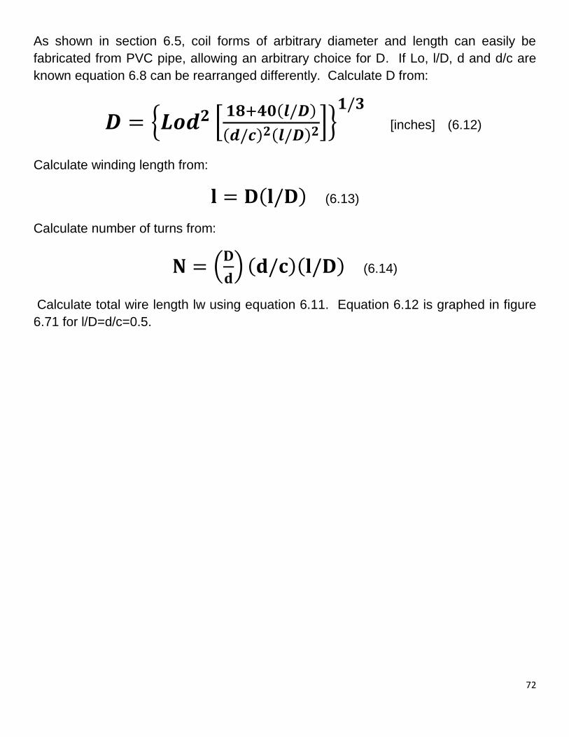
As shown in section 6.5, coil forms of arbitrary diameter and length can easily be

fabricated from PVC pipe, allowing an arbitrary choice for D. If Lo, l/D, d and d/c are

known equation 6.8 can be rearranged differently. Calculate D from:

[inches] (6.12)

Calculate winding length from:

(6.13)

Calculate number of turns from:

(6.14)

Calculate total wire length lw using equation 6.11. Equation 6.12 is graphed in figure

6.71 for l/D=d/c=0.5.

73

Figure 6.71 - Coil diameter versus Lo and wire size

74

6.10.2 Flat inductors

Lo for a flat or "pancake" winding geometry like those shown in figures 6.72 and 6.73

is:

[μH] (6.15)

Where r and t are in inches. For dimensions in cm divide eqn 6.15 by 2.54.

Figure 6.72 - Pancake winding.

Figure 6.73 - Example of a flat or pancake winding.

75

An example of the construction of a pancake winding is given in figure 6.73. Using

equation (6.15) with r=5.25", t=4" and N=59 Turns, L=1116 uH. The measured value

was L=1114 uH! Solid #12 THHN was used. The center hub was acrylic plastic and

the nine radial arms cut from 3/8" F/G electric fence wands. The winding is referred to

as "basket weave". This type of winding requires a odd number of support rods. The

self resonant frequency was ≈1.3 MHz and the QL for this inductor is shown in figure

6.74. This is quite low, primarily due to the significantly higher proximity losses

associated with this winding geometry. Inner turns lie in the fields of outer turns. On

the other hand the inductor is very compact for its inductance (1.1 mH). There may be

times when the smaller size makes the lower QL acceptable.

Figure 6.74 - Measured QL versus frequency for the pancake inductor.

76

6.10.3 toroidal inductors

Figure 6.75 - Toroidal winding example. From Terman[2].

Lo for toroidal windings like that shown in figure 6.75 is:

[μH] (6.16)

Where d' is the cross section diameter of the coil and D is the diameter of the axis of

the coil.

6.10.4 Some practical concerns

Wheeler's equation is the basis for much of the analysis in this chapter but we have to

understand it's limitations. Besides self-resonance there is always the problem of

"manufacturing tolerances", i.e. what actually gets built versus the initial design. For

example, we might want to use #12 wire with a diameter of 0.081" and have a center-

to-center spacing ratio (d/c) of 0.5. This means that c=0.162". that's not a very

convenient value when winding many turns. We are more likely to use 0.160", 0.170"

or even 0.200" for c because it's much easier to replicate especially if we're cutting

slots in a coil form.

Another problem in calculating Lo arises from the shape of the coil form. Wheeler's

equation assumes a uniform circular cylindrical coil. In practice we might use a

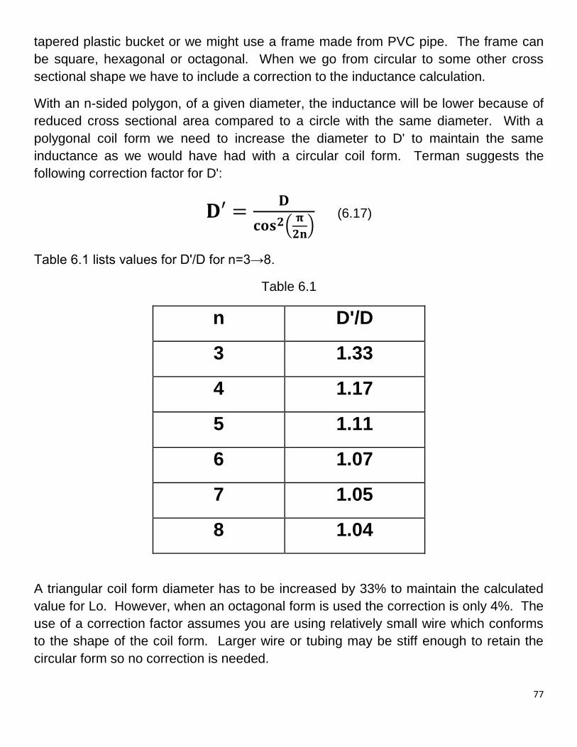
77

tapered plastic bucket or we might use a frame made from PVC pipe. The frame can

be square, hexagonal or octagonal. When we go from circular to some other cross

sectional shape we have to include a correction to the inductance calculation.

With an n-sided polygon, of a given diameter, the inductance will be lower because of

reduced cross sectional area compared to a circle with the same diameter. With a

polygonal coil form we need to increase the diameter to D' to maintain the same

inductance as we would have had with a circular coil form. Terman suggests the

following correction factor for D':

(6.17)

Table 6.1 lists values for D'/D for n=3→8.

Table 6.1

n D'/D

3 1.33

4 1.17

5 1.11

6 1.07

7 1.05

8 1.04

A triangular coil form diameter has to be increased by 33% to maintain the calculated

value for Lo. However, when an octagonal form is used the correction is only 4%. The

use of a correction factor assumes you are using relatively small wire which conforms

to the shape of the coil form. Larger wire or tubing may be stiff enough to retain the

circular form so no correction is needed.

78

Possibly the exact value needed to resonate the antenna may not be known in

advance! If the antenna has already been built and an accurate measurement of the

input impedance is available, the value for L will known but the necessary instrument

may not be available or the antenna may not yet have been built! With careful

modeling we can get a good estimate of the value for L within ≈5-10% depending on

how close the model is to the actual antenna. As was shown in chapter 3, an

approximate value for L can be calculated from antenna dimensions. Even if we

measure the input impedance with a VNA that measurement is only at one particular

time! The short heavily loaded verticals used at LF-MF have high Q's, i.e. very narrow

bandwidths[3] and are very prone to detuning, particularly as the seasons change from

dry to wet and back again. The shunt capacitance of the antenna will change with soil

conductivity which changes with moisture content. This change in shunt capacitance

will detune the antenna requiring some adjustment of L.

These observations should not be taken as gloom-and-doom! There's a simple way to

deal with these problems:

make the inductance larger than the original estimate and then tap, prune

or adjust the inductor to make final adjustments.

Besides tapping, there are other options for adjusting inductance as outlined in section

6.6. As a practical matter most tuning inductors will have to be adjustable to some

extent.

Tap placement

Coil taps will probably be needed for final tuning at the antenna but locating taps

requires some thought. When l and D are constant, L is proportional to N2. However,

when you are adding/removing turns or moving between taps the rate of change of L

will vary from ∝N2 to ∝N because you're changing both N and l.

[μH] (6.18)

Using equation 6.18 the graph in figure 6.76 was created to illustrate how L changes

with N. For this example D=3" and the winding uses #18 wire (d=0.040"). N is varied

from 5 to 100 turns for d/c=0.9 (closely wound) and d/c=0.1 (very sparse winding). The

dashed lines indicate slopes ∝N and ∝N2. With 100 turns, d/c=0.9→l=5" and

d/c=0.1→l=40". For small N the rate of change of L is close to N2 but as more turns

are added the rate of change decreases approaching ∝N for N=100. d/c=0.1 is a very

79

long coil (40") with well separated turns (c=0.4"), in this inductor L∝N except at the low

end. This behavior is something to keep in mind when selecting tap locations.

Figure 6.76 - Inductance versus turns number for fixed turn spacing.

80

6.11 Skin and proximity effects

Figure 6.77 - Skin (a) and proximity effects (b).

In an air core inductor most of the loss will be due to winding resistance (RL). As we

transition from DC to higher frequencies, RL increases! This is caused by: skin effect,

proximity effect and self-resonance. The current flowing in the conductor and the

magnetic fields associated with these currents are the source of skin and proximity

effects is as indicated in figure 6.77. The dashed lines represent magnetic field lines

resulting from the current flowing in the conductor. The solid lines represent currents

induced in the conductor. Skin effect is present in an isolated conductor and in a

winding. Proximity effect is present whenever multiple wires are close together as in a

winding.

In the following discussion the term "skin depth" will be used frequently so we need to

define what that term means. When a plane wave encounters a conducting surface

the wave will penetrate but is rapidly attenuated as indicated in figure 6.78. The

distance into the conductor where the wave amplitude is reduced by 1/e or ≈37% is

defined as the skin depth or δ. Note, e is the mathematical constant 2.718.

81

Figure 6.78

The skin depth (δ), in meters, is expressed by:

[m] (6.19)

Where:

σ is the conductivity in [Siemens/m].

μ is the permeability of the material which for Cu and Al =4πx10-7 [H/m].

f is the frequency [Hz].

The skin depth in mils for copper is:

[mils] (6.20)

At 137 kHz δ=7.03 mils (0.00703") and at 475 kHz δ=3.78 mils (0.00378").

82

6.11.1 Winding Resistance (RL)

RL can be represented by the product of the DC resistance (Rdc), a factor attributed to

skin effect (Ks) and a second factor associated with proximity effect (Kp).

(6.21)

Where:

[Ω] (6.22)

Aw is the wire cross sectional area and σ is the conductivity in S/m. lw, Aw and σ must

be in compatible units which for σ in S/m would be meters! You can also find Rdc from

a wire table where Rdc is typically listed in Ohms per thousand feet. Skin and

proximity effect terms assume a solid conductor but they can also be used for tubular.

For a tubular conductor, with a wall thickness >2δ, assume the conductor is solid, i.e.

Aw=πd2/4. This assumption works because the current in both solid and tubular

conductors of practical sizes will be concentrated in a very thin layer on the outside

perimeter. All that matters is the circumference and δ .

6.11.2 Skin depth factor Ks

As the frequency is increased the current in a conductor tends concentrate near the

surface as shown in figures 6.79 and 6.80. If we draw a line across the conductor and

measure the current density (J) we get a result like that shown in figure 6.80 where J is

very large near the surface but negligible in the interior. In effect only a small portion of

the conductor cross section conducts current which means the effective resistance is

much larger. This effect is illustrated in table 6.2 which has values for Ks at 630m and

2200m for wire sizes commonly used in tuning inductors. For example, at 475 kHz the

resistance of a #12 wire is almost six times the value at DC. This illustrates why we

must take skin effect into account.

83

Figure 6.79 - Current density in a conductor.

Figure 6.80 - Current density on a line across the conductor.

84

Table 6.2 - Ks for common wire sizes.

137 kHz 475 kHz

Wire # Ks Ks

8 4.82 8.76

10 3.87 7.00

12 3.10 5.6

14 2.53 4.49

16 2.06 3.61

18 1.15 1.93

The d/ δ ratio for common wire sizes is summarized in table 6.3.

Table 6.3 -Wire diameters in skin depths (d/δ)

frequency= 137 kHz 475 kHz

Wire # d [mils] d/δ d/δ

8 128.5 18.28 34.04

10 101.9 14.50 26.99

12 80.08 11.39 21.21

14 64.1 9.12 16.98

16 50.8 7.23 13.46

18 40.3 5.73 10.68

A general expression for the skin effect factor Ks for an arbitrary conductor diameter

can be complicated but we can see from table 6.3 for the wire sizes typically used in

tuning inductors d/δ> 5. When d/δ> 5, Ks becomes a linear function of d/δ which can

be closely approximated with a simple expression:

(6.23)

which is graphed in figure 6.81. Note that Ks is only a function of the wire diameter, d,

and skin depth (δ) at the frequency of interest.

85

Figure 6.81- Skin effect factor Ks versus wire diameter in skin depths (d/δ).

6.11.3 Proximity effect factor Kp

Figure 6.82 is a sketch of the magnetic field in a coil. The field has two components,

axial and radial, both of which affect the current distribution within the conductors. This

effect is shown by the current crowding displayed in figure 6.83. Figure 6.83 is a cross

section of a single turn but is representative of current in all the turns. Note, the left

side of figure 6.83 is the inside of the coil. Comparing figure 6.83 to figure 6.79, we

see the current is not only concentrated near the surface but is also pushed towards

the inside surface of the coil so that even less of the conductor cross section is used.

One of the earliest calculations for proximity effect, Kp, was done by S. Butterworth[4] in

1926. This analysis was accepted as gospel for many years and enshrined in

Terman[2] for generations of engineers. However, in 1947 R. Medhurst[5] fabricated and

measured 40 inductor samples discovering that there could be significant errors using

the Butterworth analysis.

86

Figure 6.82- General picture of magnetic fields in a coil.

Figure 6.83 - Cross section of a single turn on one side of a coil.

87

Despite this discovery no better analysis was published for the next 60 years!

Fortunately in the past few years Alan Payne, G3RBJ[6], has derived a new analysis

with predictions that agree well with Medhurst and I have chosen to use his analysis.

Unfortunately, as shown in section 6.11.4, the equations for Kp are much more

complicated than for Ks with no simple approximations. However, graphs and tables

for Kp, with sufficient accuracy for our purposes, can be generated using Alan's

equations.

Proximity factor, Kp, is a function of:

d/c - the turn-to-turn spacing ratio

l/D - the length/diameter ratio

N - the number of turns in the winding

The spacing ratio matters because the interaction between turns increases as spacing

is reduced. The effect of l/D is not quite so obvious. Figure 6.82 indicates there are

two components to the field within the coil: radial and axial. The loss due to the radial

component occurs largely at the ends of the coil where the field diverges whereas the

axial loss is distributed over the entire coil. For a long skinny coil (large l/D) the loss at

the ends is a smaller part of the total loss. However, for a large diameter with a short

winding (small l/D) most of the loss is near the ends. This is one of the reasons why

d/c and l/D are prominent in many inductor calculations.

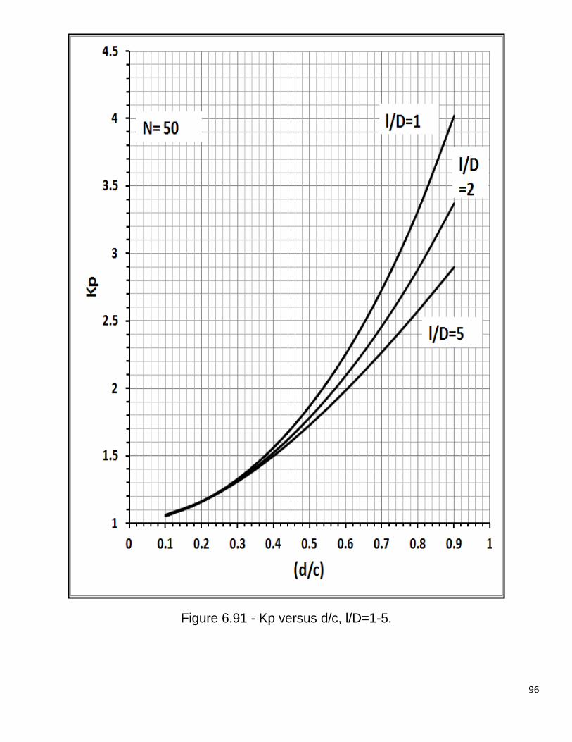
Figures 6.84 and 6.85 show values for Kp as a function of l/D with N as a parameter.

0.3< d/c < 0.9 represents the usual range for d/c. Note that for N≥30 turns Kp does not

vary greatly with N. This is important because it allows us to use either a single graph

or a single table for Kp which simplifies things. Usually the graph or table for N=50 is

chosen as a compromise since tuning inductors will typically have >30 turns. In any

case when N is <30 using the N=50 graph leads to a small overestimate of Kp.

Table 6.4. is a table of Kp values for a range of values of l/D and d/c. Figures 6.86-

6.92 provide more information on Kp. As l/D is increased Kp initially increases peaking

at l/D≈0.75. Beyond that point Kp decreases. This tells us that if we want low RL,

which implies high Q, we should consider using l/D ratios well below or above 0.75.

This ties in with figure 6.5 (in Part l) which shows that l/D=0.45 gives the largest value

for L. The graphs also show that Kp is very sensitive to d/c, increasing rapidly as the

turn-to-turn spacing is decreased for a give wire size. Well spaced turns would appear

to work best. In practice coils with l/D=0.5 and d/c=0.5 are usually a good

compromise.

88

Figure 6.84 -Kp as a function of l/D and N with d/c=0.3.

89

Figure 6.85 - Kp as a function of l/D and N with d/c=0.9.

90

Table 6.4 - Values for proximity factor Kp, N≥30 turns.

(d/c)= 0.1 0.2 0.3 0.4 0.5 0.6 0.7 0.8 0.9

l/D Kp Kp Kp Kp Kp Kp Kp Kp Kp

0.3 1.03 1.10 1.22 1.39 1.62 1.92 2.31 2.80 3.42

0.4 1.03 1.12 1.25 1.45 1.72 2.06 2.51 3.06 3.75

0.5 1.04 1.13 1.28 1.49 1.78 2.16 2.63 3.22 3.95

0.6 1.04 1.14 1.30 1.52 1.82 2.21 2.70 3.31 4.06

0.7 1.05 1.15 1.31 1.54 1.85 2.24 2.74 3.35 4.10

0.8 1.05 1.15 1.32 1.55 1.86 2.26 2.75 3.36 4.10

0.9 1.05 1.15 1.32 1.56 1.87 2.26 2.75 3.35 4.07

1 1.05 1.16 1.33 1.56 1.87 2.25 2.73 3.32 4.02

1.1 1.05 1.16 1.33 1.56 1.86 2.24 2.71 3.28 3.96

1.2 1.05 1.16 1.33 1.56 1.85 2.23 2.68 3.23 3.89

1.3 1.05 1.16 1.32 1.55 1.85 2.21 2.65 3.18 3.81

1.4 1.05 1.16 1.32 1.55 1.84 2.19 2.62 3.14 3.74

1.5 1.05 1.16 1.32 1.54 1.83 2.17 2.59 3.09 3.67

1.6 1.06 1.16 1.32 1.54 1.82 2.16 2.56 3.04 3.60

1.7 1.06 1.16 1.32 1.53 1.81 2.14 2.53 3.00 3.54

1.8 1.06 1.16 1.32 1.53 1.80 2.12 2.51 2.96 3.48

1.9 1.06 1.16 1.32 1.53 1.79 2.11 2.48 2.92 3.42

2 1.06 1.16 1.31 1.52 1.78 2.09 2.46 2.88 3.37

91

Figure 6.86 - Kp versus l/D with N=10.

92

Figure 6.87 - Kp versus l/D with N=20.

93

Figure 6.88 - Kp versus l/D with N=30.

94

Figure 6.89 - Kp versus l/D with N=50.

95

Figure 6.90 -Kp versus d/c, l/D=0.3-0.7.

96

Figure 6.91 - Kp versus d/c, l/D=1-5.

97

Figure 6.92 -Kp versus N for d/c=0.2-0.9.

98

6.11.4 Summary of Payne Kp equations

Where:

99

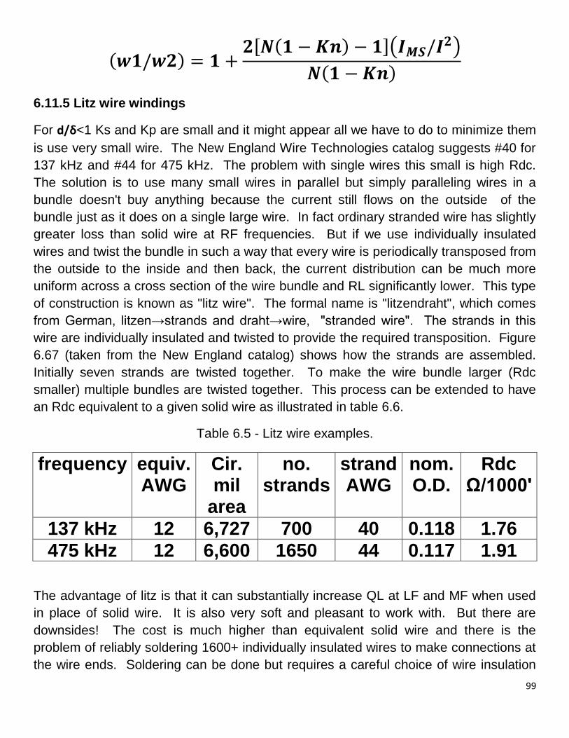
6.11.5 Litz wire windings

For d/δ<1 Ks and Kp are small and it might appear all we have to do to minimize them

is use very small wire. The New England Wire Technologies catalog suggests #40 for

137 kHz and #44 for 475 kHz. The problem with single wires this small is high Rdc.

The solution is to use many small wires in parallel but simply paralleling wires in a

bundle doesn't buy anything because the current still flows on the outside of the

bundle just as it does on a single large wire. In fact ordinary stranded wire has slightly

greater loss than solid wire at RF frequencies. But if we use individually insulated

wires and twist the bundle in such a way that every wire is periodically transposed from

the outside to the inside and then back, the current distribution can be much more

uniform across a cross section of the wire bundle and RL significantly lower. This type

of construction is known as "litz wire". The formal name is "litzendraht", which comes

from German, litzen→strands and draht→wire, "stranded wire". The strands in this

wire are individually insulated and twisted to provide the required transposition. Figure

6.67 (taken from the New England catalog) shows how the strands are assembled.

Initially seven strands are twisted together. To make the wire bundle larger (Rdc

smaller) multiple bundles are twisted together. This process can be extended to have

an Rdc equivalent to a given solid wire as illustrated in table 6.6.

Table 6.5 - Litz wire examples.

frequency equiv. AWG

Cir. mil

area

no. strands

strand AWG

nom. O.D.

Rdc Ω/1000'

137 kHz 12 6,727 700 40 0.118 1.76

475 kHz 12 6,600 1650 44 0.117 1.91

The advantage of litz is that it can substantially increase QL at LF and MF when used

in place of solid wire. It is also very soft and pleasant to work with. But there are

downsides! The cost is much higher than equivalent solid wire and there is the

problem of reliably soldering 1600+ individually insulated wires to make connections at

the wire ends. Soldering can be done but requires a careful choice of wire insulation

100

and technique. Those interested in using litz should go to the wire manufactures

catalogs and applications notes.

Figure 6.93 - Examples of litz construction.

101

Litz wire can be useful but we cannot use just any litz. Michael Perry[7] has published a

formal analysis of litz wire construction which contains a cautionary tale!

Figure 6.94 - Rac comparison between solid and litz wire. From Perry[7].

Figure 6.94 is taken from Perry. The wire diameter is in skin depths. It compares Rac

between a solid conductor and a litz conductor which varies with the size of the

individual wires (d/δ) or when the frequency is changed. Litz can have a small number

of wires and only a few layers or many wires forming many layers. In general the more

layers and the smaller the individual strands the greater the improvement. However,

there is a trap here! The reduction in Rac occurs only over a small range of wire sizes

102

at a given frequency or, for a given wire size, over only a narrow range of frequencies.

The key point shown in this graph is:

If the individual wire size is too large or equivalently if the frequency is

higher than the minimum Rac point, Rac can be much higher using litz than

in an equivalent solid wire!

The following quotation from Perry should be taken to heart if you are considering litz

wire:

"The foregoing analysis indicates some surprising design results which

may directly contradict widely held beliefs regarding ac resistance in wires

and cables. For example, suppose a solid conductor is excited at a certain

frequency which results in a radius which is many times the skin-depth.

Then, assume a designer switches to a cable of the same total diameter but

with several layers of stranded wire to reduce losses such that d/δ>2. By

inspection of Fig. 6.94, this process can result in far greater losses than if

the "solid" conductor were employed. Stated another way, an uninformed

design of Litz wire can result in a performance characteristic which is

much worse than if nothing at all were done to reduce losses!

A second and important fact is that the cross-sectional area of a cable

comprising stranded wires is substantially reduced from the conducting

area of a "solid" cable of the same radius. This is due to the fact that each

strand is usually round and insulated with a varnish or other

nonconductor. The round insulated wires in the cable yield a "packing

factor" which reduces the conducting area by a significant fraction, usually

at least 40 percent. The transposition process further reduces the cross-

sectional area available for carrying current. The final result is a

substantial reduction the net savings available in ac resistance by utilizing

Litz wire. Due to these limitations, the Litz wire principle for reducing ac

losses must be thoroughly understood in the context of a specific

application before it should be employed."

Enough said!

103

6.12 Self resonance

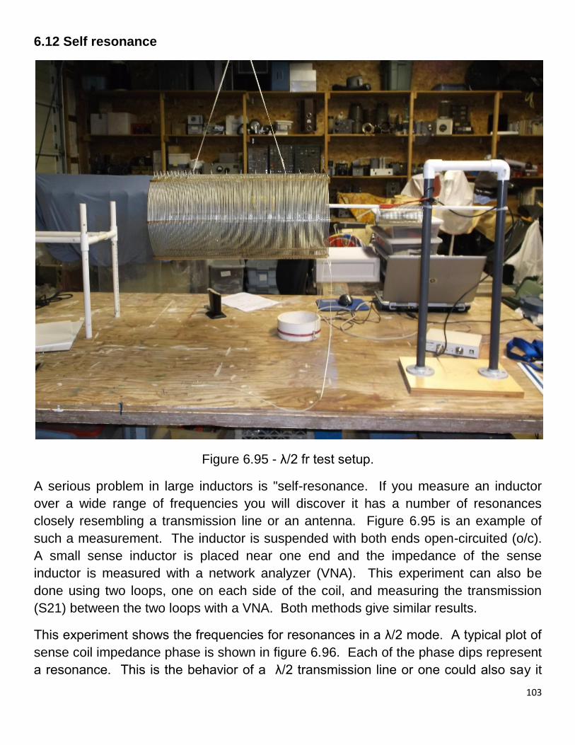
Figure 6.95 - λ/2 fr test setup.

A serious problem in large inductors is "self-resonance. If you measure an inductor

over a wide range of frequencies you will discover it has a number of resonances

closely resembling a transmission line or an antenna. Figure 6.95 is an example of

such a measurement. The inductor is suspended with both ends open-circuited (o/c).

A small sense inductor is placed near one end and the impedance of the sense

inductor is measured with a network analyzer (VNA). This experiment can also be

done using two loops, one on each side of the coil, and measuring the transmission

(S21) between the two loops with a VNA. Both methods give similar results.

This experiment shows the frequencies for resonances in a λ/2 mode. A typical plot of

sense coil impedance phase is shown in figure 6.96. Each of the phase dips represent

a resonance. This is the behavior of a λ/2 transmission line or one could also say it

104

behaves like the λ/2 resonances in a dipole antenna. There has been some discussion

on how to characterize these resonances: as a transmission line or as a standing wave

structure like an antenna. Either view seems to agree with observation.

Figure 6.96 - Phase of probe impedance, λ/2 resonances.

We can run a similar test with one end of the inductor grounded to a large plate to

determine the resonances in the λ/4 mode which is the normal mode for an inductor in

a circuit. Figure 6.97 shows a transmission line representation with some parasitic

loading capacitance (Cp). As a circuit element the inductor behaves much like a s/c

λ/4-wave transmission line or a λ/4 vertical antenna.

105

Figure 6.97 - Inductor-transmission line analogy.

Dave Knight, G3YNH[8], conducted a very ingenious experiment, shown in figure 6.98.

A coil was excited near resonance using a loop connected to a transmitter.

Figure 6.98 -G3YNH coil with excitation, λ/2-resonance. Courtesy of G3YNH.

106

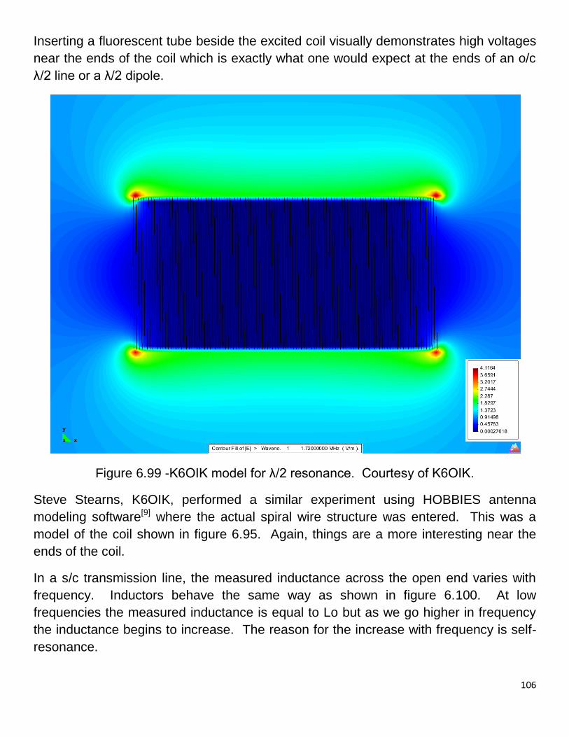
Inserting a fluorescent tube beside the excited coil visually demonstrates high voltages

near the ends of the coil which is exactly what one would expect at the ends of an o/c

λ/2 line or a λ/2 dipole.

Figure 6.99 -K6OIK model for λ/2 resonance. Courtesy of K6OIK.

Steve Stearns, K6OIK, performed a similar experiment using HOBBIES antenna

modeling software[9] where the actual spiral wire structure was entered. This was a

model of the coil shown in figure 6.95. Again, things are a more interesting near the

ends of the coil.

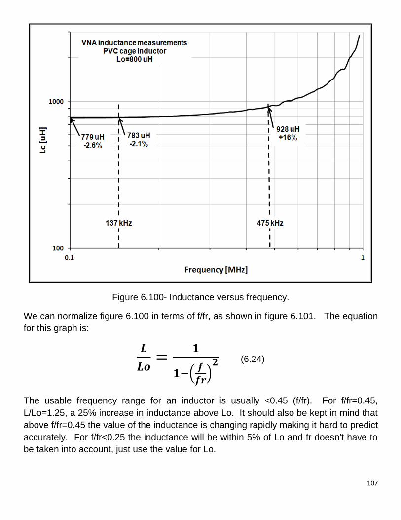
In a s/c transmission line, the measured inductance across the open end varies with

frequency. Inductors behave the same way as shown in figure 6.100. At low

frequencies the measured inductance is equal to Lo but as we go higher in frequency

the inductance begins to increase. The reason for the increase with frequency is self-

resonance.

107

Figure 6.100- Inductance versus frequency.

We can normalize figure 6.100 in terms of f/fr, as shown in figure 6.101. The equation

for this graph is:

(6.24)

The usable frequency range for an inductor is usually <0.45 (f/fr). For f/fr=0.45,

L/Lo=1.25, a 25% increase in inductance above Lo. It should also be kept in mind that

above f/fr=0.45 the value of the inductance is changing rapidly making it hard to predict

accurately. For f/fr<0.25 the inductance will be within 5% of Lo and fr doesn't have to

be taken into account, just use the value for Lo.

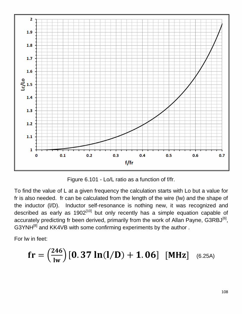
108

Figure 6.101 - Lo/L ratio as a function of f/fr.

To find the value of L at a given frequency the calculation starts with Lo but a value for

fr is also needed. fr can be calculated from the length of the wire (lw) and the shape of

the inductor (l/D). Inductor self-resonance is nothing new, it was recognized and

described as early as 1902[10] but only recently has a simple equation capable of

accurately predicting fr been derived, primarily from the work of Allan Payne, G3RBJ[6],

G3YNH[8] and KK4VB with some confirming experiments by the author .

For lw in feet:

(6.25A)

109

For lw in meters:

(6.25B)

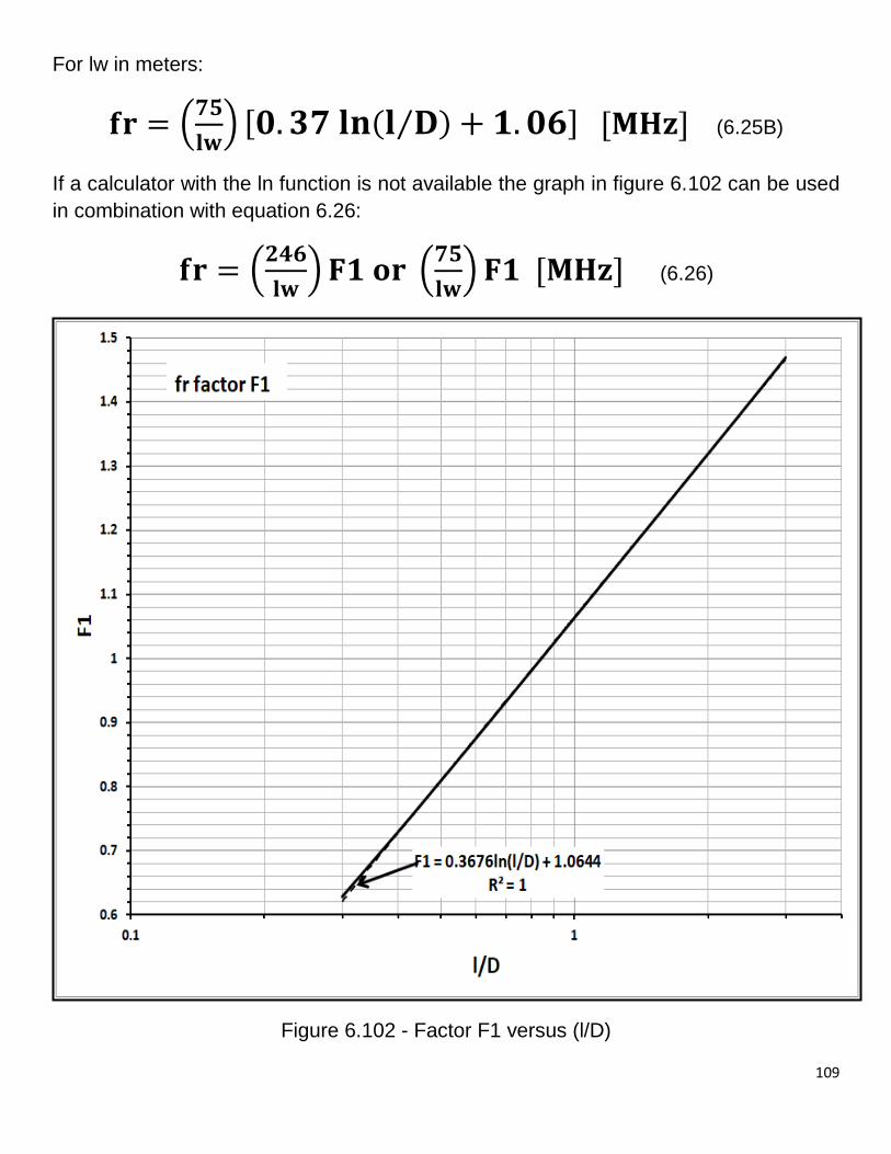
If a calculator with the ln function is not available the graph in figure 6.102 can be used

in combination with equation 6.26:

(6.26)

Figure 6.102 - Factor F1 versus (l/D)

110

Note, F1 increases substantially with increasing l/D. This indicates that using higher

values for l/D will increase fr. Also notice in equations 6.25 and 6.26, there are only

two variables: the length of the wire (lw) and the length-diameter ratio (l/D) of the coil.

To this point the fr discussion has assumed an air wound coil with no insulation on the

wires. However, there will be many occasions where a plastic coil form (bucket or PVC

pipe) may be used. In addition windings often use insulated wire such as THHN house

wiring which has PVC insulation. These are dielectric materials with relative dielectric

constants (Er, relative permittivity) greater than one. The velocity v of a wave in a

dielectric material will be:

(6.27A)

For most dielectrics uo=1, so eqn 6.27A reduces to:

(6.27B)

Where c is the speed of light.

The winding is a transmission line and the electrical length of a transmission line

depends on v . The result is that the self-resonant frequency with a dielectric (fr')

becomes:

(6.28)

i.e. the self-resonant frequency will be lower in proportion to the square root of the

relative permittivity.

The result of placing dielectric materials in close proximity to the winding creates an effective Er which is an average, lower than that of the wire insulation or the coil form but greater than air. This can be demonstrated using the Q measurements shown earlier in section 6.5 and shown again in figure 6.103 In this example fr=1255 kHz and fr'=1000 kHz, which implies Er=(fr/fr')2≈1.575 which is smaller than the Er for PVC but still greater than one resulting in a significant downward shift in fr. Q is reduced from ≈620 to ≈550! Even a small air-gap between the turns reduces the effective Er, increasing fr. Winding coils with insulated wire and a small air gap between the turns is discussed in section 6.5.

111

Figure 6.103 - Comparison between tight and loose windings.

Equations 6.25 and 6.26 are for an ideal inductor far removed from ground, conducting

objects, etc. In any practical installation some parasitic shunt capacitance (indicated in

figure 6.96) will be introduced by the associated circuit wiring and/or a metal enclosure

and/or proximity to ground. This usually means fr will be somewhat lower than

calculated which is another reason for not pushing the f/fr ratio too high.

112

6.13 Q

The Q of an inductor is defined by:

(6.29)

Where Q, L and RL represent values taking into account Ks, Kp and fr.

Figure 6.104 - Effect of wire size on Q with d/c=l/D=0.5.

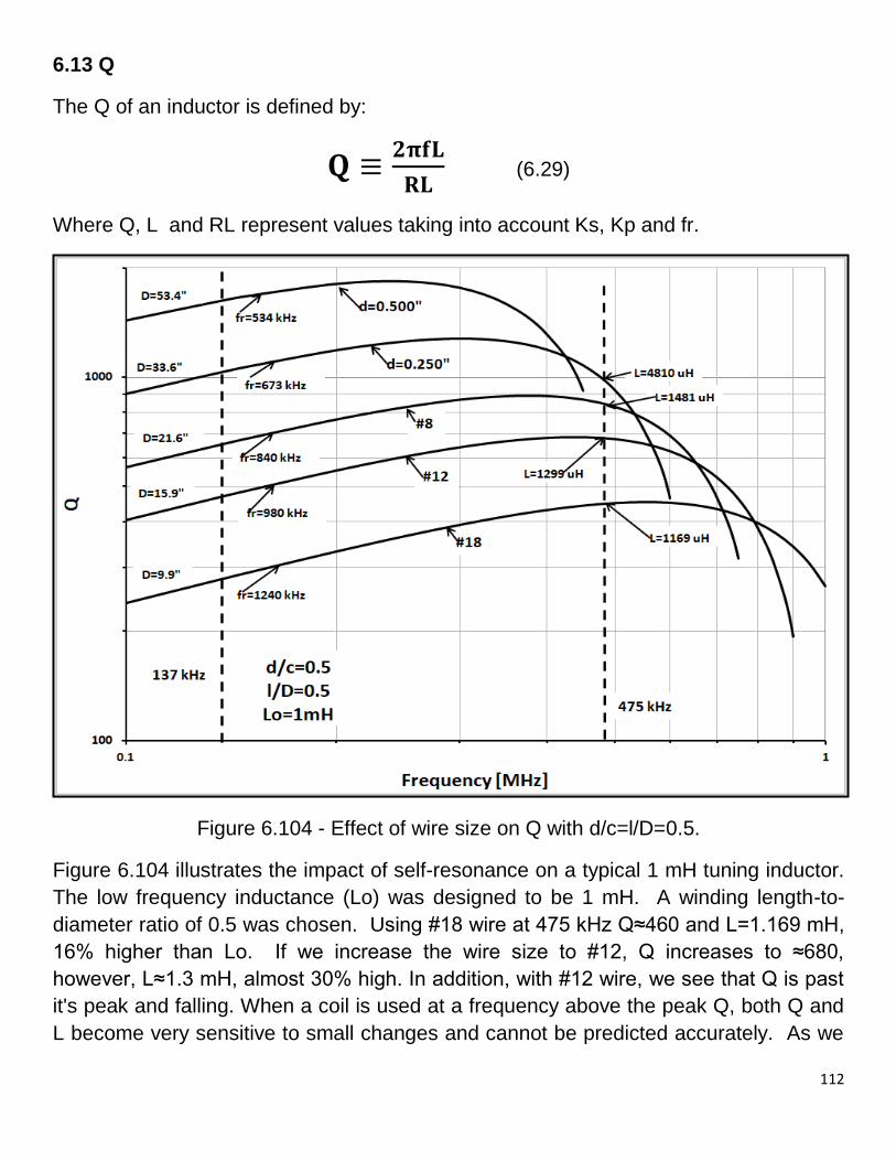
Figure 6.104 illustrates the impact of self-resonance on a typical 1 mH tuning inductor.

The low frequency inductance (Lo) was designed to be 1 mH. A winding length-to-

diameter ratio of 0.5 was chosen. Using #18 wire at 475 kHz Q≈460 and L=1.169 mH,

16% higher than Lo. If we increase the wire size to #12, Q increases to ≈680,

however, L≈1.3 mH, almost 30% high. In addition, with #12 wire, we see that Q is past

it's peak and falling. When a coil is used at a frequency above the peak Q, both Q and

L become very sensitive to small changes and cannot be predicted accurately. As we

113

increase the wire size Q increases but at 475 kHz the Q is well past it's peak value and

falling rapidly. The inductance is also much larger and changing rapidly. What this

example shows is the maximum value for Q is limited to ≈650 and the analysis, which

is relatively simple for Lo, becomes more complex.

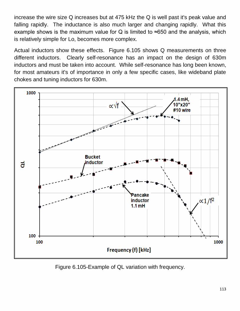
Actual inductors show these effects. Figure 6.105 shows Q measurements on three

different inductors. Clearly self-resonance has an impact on the design of 630m

inductors and must be taken into account. While self-resonance has long been known,

for most amateurs it's of importance in only a few specific cases, like wideband plate

chokes and tuning inductors for 630m.

Figure 6.105-Example of QL variation with frequency.

114

Equation 6.29 can be manipulated into a form which allows us to predict the variation

of Q in terms a known low frequency Q=Q1 and fr:

(6.30A)

Equation 6.25A can be rearranged to create a graph of Q versus f normalized to fr:

(6.30B)

Q1=Q at a given frequency f1:

(6.31)

Where RL1 is the value for RL at f1.

The quantity F in equation 6.30B is graphed in figure 6.106 where the dashed line

represents the behavior of Q when self-resonance is not present. The solid line

illustrates the effect of self-resonance. Note that the maximum point for F, which

corresponds to maximum Q, occurs at f/fr≈0.45, roughly half the self-resonant

frequency. Given that we are concerned with 630m and 2200m, the minimum

allowable values for fr can be given in a table.

Table 6.6 - Minimum values for fr

band fr, minimum L error %

0.20fr 475 kHz 2375 kHz +4

0.25fr 475 kHz 1900 kHz +6.7

0.30fr 475 kHz 1583 kHz +10

0.45fr 475 kHz 1056 kHz +25

0.20fr 137 kHz 685 kHz +4

0.25fr 137 kHz 548 kHz +6.7

0.30fr 137 kHz 457 kHz +10

0.45fr 137 kHz 304 kHz +25

115

Figure 6.106 - F-factor versus f/fr.

Table 6.6 gives some very important information. If we are willing to accept an error in

L ≤10%, we can allow f/fr up to 0.3. Values of f/fr≤0.3 allow us to use a much simpler

design procedure omitting fr considerations. The question now is how do we know

which design procedure to use? We can rearrange equation 6.25 to show the

maximum value for lw for a given minimum fr:

(6.32)

Peak Q occurs at 0.45fr and we will want that peak at or above 475 kHz, i.e. fr≥1055

kHz or at 137 kHz, fr≥304 kHz. A graph showing the maximum usable lw at 475 and

137 kHz for f/fr=0.30 and 0.45 is shown in figure 6.107.

116

Figure 6.107 - Maximum lw, limited by self-resonance.

Figure 6.107 is helpful but it's even more helpful to know the limits on Lo? To resolve

that question Wheelers equation for Lo can be rearranged into a form which includes

lw,max, l/D, d and d/c:

(6.33)

Figure 6.108 is a graph of using equation 6.33 showing the maximum Lo for which we

can ignore fr when using #12 wire. d/c=0.3 represents case where the proximity loss is

low. d/c=0.7 is a typical value for a coil with closely wound THHN or other insulated

wire.

117

Figure 6.108 - Maximum values for Lo [uH].

118

6.13.1 Verification

Before using the design equations presented we need to answer a very basic question:

"do the equations presented in preceding sections actual work and if so, how well?"

One way to answer this is to compare Q measurements on existing inductors against

calculated predictions.

Figure 6.109- Q measurement setup.

The basic tool for this is a Q-meter, for this work an HP4342A Q-meter was used.

Figure 6.109 is an example of the experimental setup. Two inductors were measured

and calculated with the results shown in figures 6.111 and 6.112.

The first example was a commercial broadcast transmitter inductor shown in figure

6.110 where d=#10, D≈10", l≈20" and d/c≈0.6. The second example was a home-brew

inductor using a PVC pipe cage for the coil form shown in figure 6.38.

119

Figure 6.110 - Large commercial BC inductor.

For the BC inductor: at 137 kHz QL≈450 and at 475 kHz QL≈690. This is quite a good

inductor but it should be noted that it's form (l/D and d/c) is not quite optimum. Using

the same length of wire and rewinding with a more optimum l/D and d/c, a Q

approaching 1000 would be possible. In both examples the agreement between

prediction and measurement is very close. The equations presented in preceding

sections work!

120

Figure 6.111 - BC coil Q measurements and predictions.

121

Figure 6.112 - Measured (dots) versus calculated QL (dashed line).

122

6.13.2 Maximizing Q

Because of the impact inductor losses have on antenna efficiency, obtaining as high a

Q as practical is important. This section is focused on maximizing Q. As preceding

sections have shown, there are several effects limiting achievable Q: skin effect,

proximity effect and self-resonance. These in turn are functions of frequency, desired

inductance and dimensional variables: wire diameter (d), length-diameter ratio (l/D),

turn-to-turn spacing ratio (d/c), etc. Q is a function of some subset of variables:

(6.29)

Q optimization is challenging because it's a multi-dimensional problem! Several

variables must be juggled at once while seeking the best combination. In this section

we will try to get a good feeling for the impact of different variables on Q, suggesting

how to optimize Q.

What's the difference between 630m and 2200m?

Figure 6.113 shows an example of the dependency of Q and fr on l/D ratio in a 1mH

inductor wound with #12 wire. d/c=0.5 was chosen as a compromise between wire

length and proximity loss. At 137 kHz l/D=0.5 is the best choice, in fact a small further

improvement can be had by using l/D=0.45. As l/D is increased Q falls because

proximity loss (Kp) increases with l/D but fr increases with l/D which implies a reduction

in loss. At 137 kHz fr has very little effect and Kp dominates so minimizing l/D gives the

highest Q. But at 475 kHz fr has considerable effect and the value for Q at l/D=1 is

slightly better than for l/D=0.5 (Q≈685). Even for l/D=2 Q≈650 which is still pretty good.

There are two key points here, first optimization at 137 kHz is different than at 475 kHz

and, at 475 kHz Q may not be as sensitive to l/D because fr is the limiting factor.

Associated with figure 6.113 is figure 6.114, a graph of L (not Lo!) versus frequency.

At 137 kHz fr has little effect so L≈Lo and maximum Q corresponds to l/D=0.45.

However, at 475 kHz L >> Lo and the value for l/D matters. If a larger l/D is used, say 1

or even 2, we sacrifice some Q but in exchange we get a more stable and predicable

inductance value.

123

Figure 6.113 -Q versus frequency with l/D as a parameter.

124

Figure 6.114 - Inductance versus frequency.

Figures 6.113 and 6.114 assumed d/c=0.5, figure 6.115 shows what happens if we

vary d/c while holding l/D constant (0.5). At 137 kHz a low d/c gives higher Q but at

475 kHz a low value for d/c (0.3) is associated with a low fr which kills the Q and

makes the inductance hard to predict. Notice that Q is quite sensitive to d/c. If we

compromise by using d/c=0.6 instead of 0.5, the Q at 475 kHz drops from ≈685 to ≈620

but f/fr at 475 kHz is now <0.45.

The preceding examples assumed #12 wire but other wire sizes can be used as shown

in figure 6.116. At 137 kHz Q the wire size can be increased up to 0.5". For d=0.25"

Q>1000 and d=0.5", Q≈1700! Note however, that the diameter (D) when using 0.5"

wire (actually copper tubing!) is over 53", and with l/D=0.5, will have a winding length of

≈26". While providing a very high Q, this large inductor would be quite expensive to

build due to the cost of copper tubing!

125

Larger wire has longer lw which pushes fr well below the 1055 kHz limit for 475 kHz.

The larger wires also have a much larger values for L which is changing rapidly at 475

kHz as indicated on the graph. For a 1 mH inductor with l/D=d/c=0.5, #12 wire is about

the largest usable size. The coil diameter (D) for each wire size is also shown on the

graph. Note how physically large the inductor becomes. Up to the point where fr limits

Q, larger inductors, of a given inductance value, will usually have higher Q.

Figure 6.115 - Effect of d/c on Q.

126

Figure 6.116 - Effect of wire size on Q with d/c=l/D=0.5.

The impact of increasing l/D from 0.5 to 1 is shown in figure 6.117. Comparing 6.116

and 6.117, at 475 kHz, for #12 wire, Q goes from ≈685 to ≈720, not all that different,

but we can now use #10 wire with Q≈900 or #8 wire and reach Q≈930. In general it

will be necessary to juggle wire size, l/D, d/c and fr to get an acceptable Q and

predicable L.

One point to remember when using taps, fr does not change greatly when moving to a

lower tap on the inductor. An analog for that situation is tapping down on a

transmission line as shown in figure 6.118. fr is still determined by the total length of

the transmission line. In practice moving to a tap will shift the location of the parasitic

capacitance (Cp) and this will shift fr but usually not by very much.

127

Figure 6.117 - Effect of wire size on Q with d/c= 0.5 and l/D=1..

Figure 6.118 - Tapped transmission line model.

128

6.14 Symbols and abbreviations

Aw → cross sectional area of the winding conductor

c → center-to-center spacing between turns, winding pitch

d → diameter of the winding conductor

D → diameter of the winding

f → operating frequency

fr → self resonant frequency

Kp → proximity factor

Ks → skin effect factor

l → coil length

L→ inductance

Lo→ low frequency inductance

lw→ length of the winding conductor

Figure 6.119 - inductor dimensions

N → number of turns in the winding

129

Rdc → DC resistance of the winding conductor

RL → AC winding resistance including Rdc + skin and proximity effects

Q → inductor Q

δ → skin depth

σ → conductivity of winding conductor

The inductor design graphs and equations can be made more general with geometric

ratios as variables. For example:

(d/c) → conductor diameter/turn center-to-center spacing ratio

(l/D) → coil length/diameter ratio

References

[1] Wheeler, H.A., Simple Inductance Formulas for Radio Coils, Proceedings of the

IRE, October 1928, Vol. 16, p. 1398

[2] Terman, Frederick E., Radio Engineers Handbook, McGraw-Hill Book Company,

1943. This is a very useful book!

[3] Yaghjian and Best, Impedance, Bandwidth and Q of Antennas, IEEE transactions on Antennas and Propagation , Vol. 53, No. 4, April 2005, pp. 1298-1324

[4] S. Butterworth, Effective Resistance of Inductance Coils at Radio Frequency, The Wireless Engineer, April 1926, pp. 203-209, May 1926, pp. 309-316, July 1926, pp. 417-424, August 1926, pp. 48-492

[5] R. G. Medhurst, Resistance and Self-Capacitance of Single-Layer Solenoids, Wireless Engineer, February 1947, pp. 35-43, March 1947, pp. 80-92

[6] Alan Payne, G3RBJ, http://g3rbj.co.uk [7] Michael Perry, Low Frequency Electromagnetic Design, Marcel Dekker, Inc. 1985, pp. 107-116 [8] David Knight, G3YNH, http://www.g3ynh.info [9] HOBBIES, Higher Order Basis Based Integral Equation Solver, John Wiley and Sons, 2012, ISBN:978-1-118-14065-9

130

[10] P. Drude, Zur construction von Teslatransformatoren, Schwingungsdauer und Selbstinduction von Drahtspulen, (On the construction of Tesla transformers: period of oscillation and self-inductance of the coil), 1902 Annalen der Physic 1902. An English translation by Knight and Weaver, 2015, is available at: https://www.researchgate.net/publications/301624796 [11] Rudy Severns, N6LF, Conductors for HF Antennas, Nov/Dec 2000 QEX, pp.20-29

[12] Rudy Severns, N6LF, Insulated Wire and Antennas, QEX March/April 2018, pp.

22-28