175 Chapter 5 The High Altitude Tropical Dust

Maximum

5.1 Introduction Because it is strongly radiatively active and highly temporally and spatially variable in its

abundance, suspended dust is the martian atmosphere’s most meteorologically important

component. Indeed, the role of dust in Mars’s surface/atmosphere system is analogous to

the role of water in Earth’s surface/atmosphere system.

First, the more dynamic weather systems of Mars are chiefly associated with dust

clouds: dust devils [Thomas and Gierasch, 1985; Balme and Greeley, 2006; Cantor et al.,

2006], dust “cells” [Cantor et al., 2002], and dust storms at various scales [Kahn et al.,

1992]. Mars has carbon dioxide and water ice clouds (and the Earth has dust storms). But

these types of martian clouds generally are not associated with turbulent weather at the

surface, with the possible exception of carbon dioxide snow squall activity in polar night

[Colaprete et al., 2008].

Second, meteorological systems re-circulate dust on seasonal timescales, lifting

dust from some surfaces, precipitating them upon others, and usually re-charging the

original sources from the sinks [Szwast et al., 2006], producing a true “dust cycle.”

Surface dust is both more reflective and more swiftly heated and cooled than the dark

basaltic rock that makes up much of the planet’s surface, providing thermal contrast

between dusty “continents” and basaltic “seas” [Zurek et al., 1992].

Third, the presence of a small background dust concentration in the atmosphere,

which is heated strongly during the day in the visible and weakly cools in the infrared at

night, enhances the static stability of the atmosphere in ways not dissimilar to water

176 vapor in Earth’s denser and more humid atmosphere [Haberle et al., 1982; Schneider,

1983]. Mars even may have a form of dust related convection analogous to moist

convection due to water on the Earth. Fuerstenau [2006] proposed that dust devil plumes

(and potentially larger dust structures) might be so strongly heated by the sun during the

day that parcels within them might be strongly positively buoyant. Such parcels might

have vertical velocities of 10 ms-1 and reach heights of 8 km or more. This mechanism

might explain the great heights reached by larger martian dust devils compared to their

terrestrial analogs [Fisher et al., 2005]. The production of positive buoyancy by the solar

heating of dust also could explain the “puffy” dust clouds observed in intense dust storm

activity that have been compared to deep moist convective “hot towers” on the Earth

[Strausberg et al., 2005]. Note that this effect is distinct from the positive feedback effect

on winds within lower aspect ratio circulations due to dust heating [Haberle et al., 1993],

which does not require positive buoyancy or result in large vertical velocities.

Fourth, the contribution of dust to the lower atmospheric heat budget also has a

water-related terrestrial analog. In Chapter 4, I calculated that the tropical zonal average

atmospheric mass heating rates on Mars due to dust under relatively clear conditions are

similar to or greater than tropical mass heating rates due to moist convective latent heat

release on the Earth. Thus, if Earth is a planet defined by its hydrometeorology (“water

weather”), Mars is defined by its coniometeorology (“dust weather”), the latter word

being derived from the Greek word for dust, konios.

Accurate simulation of Mars’s modern circulation, past climate, and future

weather therefore is dependent on understanding the connection between the synoptic and

mesoscale systems that lift and transport dust and the resulting distributions of airborne

177 and surface dust. Modelers of the martian atmosphere have explored this connection

in considerable detail, simulating dust lifting and transport with more or less

parameterized routines in planetary and mesoscale models [e.g., Murphy et al., 1990;

Newman et al., 2002a, 2002b; Richardson and Wilson, 2002; Rafkin et al., 2002; Basu et

al., 2004, 2006; Kahre et al., 2005, 2006, 2008].

Several datasets have been used to tune or verify these simulations. These datasets

fall into two broad types: (1) nadir column opacity measurements from the surface or

orbiters and (2) temperature measurements from orbit, particularly the brightness

temperature near the center of the 15 micron CO2 band, T15 [e.g., Newman et al., 2002a;

Basu et al., 2004]. The first type of measurement is more sensitive to dust near the

surface than dust high in the atmosphere, even though the dust high in the atmosphere

still can produce significant radiative heating and cooling. The second type of

measurement is more sensitive to finer aspects of the vertical structure of the dust

distribution but also can be influenced by dynamical processes indirectly driven by or

independent of dust heating phenomena such as water ice clouds, especially if

atmospheric dust concentrations are relatively low. The logical alternative to these

verification measurements is more direct observation of the vertical dust distribution

through infrared or visible limb sounding.

Vertical profiles of temperature, pressure, dust, and other aerosol retrieved from

observations by the Mars Climate Sounder (MCS) on Mars Reconaissance Orbiter

(MRO) now provide an expansive dataset [McCleese et al., 2007, 2008; Kleinböhl et al.,

2009] for observing the vertical structure of Mars’s coniometeorological systems,

178 evaluating present simulations of dust lifting and transport, and indicating avenues for

improvement of the parameterizations used to drive these simulations.

This study is very much a first step in using the abundance of retrieved vertical

profiles of dust from MCS observations to improve understanding of Mars’s

coniometeorology. Chapter 4 showed that the vertical and latitudinal dust distribution of

Mars in northern spring and summer was very different from that generally assumed,

especially by general circulation models forced by prescribed dust concentrations. The

most discrepant feature is an apparent maximum in dust mass mixing ratio over the

tropics during most of northern spring and summer, “the high altitude tropical dust

maximum” (HATDM).

In this study, the HATDM is investigated in greater detail than Chapter 4 in order

to determine its cause. In Chapter 5.2, the observed MCS dust distributions at northern

summer and southern summer solstices are compared with planetary-scale simulations of

active lifting and transport. In Chapter 5.3, the longitudinal structure of the HATDM and

its temporal variability is investigated. In Chapter 5.4, the potential roles of dust storm

activity, orographic dust lifting, pseudo-moist dust convection, and the scavenging of

dust particles by water ice clouds in producing the HATDM are evaluated, and I outline

what further observations and modeling work are necessary to constrain the contributions

of these processes. In Chapter 5.5, I summarize the results of the study.

179 5.2 Comparison of MCS Vertical Dust Profiles with

Simulations of Active Lifting and Transport

A number of Mars GCMs now have the capability to simulate the lifting,

sedimentation, and horizontal transport of dust in Mars’s atmosphere. Most modeling

studies, however, have focused on the simulation of global dust storms and therefore do

not describe the simulated latitudinal and vertical distribution of dust during the clear

season. Two exceptions are Richardson and Wilson [2002], which uses the Mars GFDL

model, and Kahre et al. [2006], which uses the Ames Mars GCM.

Figures 5.1a and 5.1b plot the nightside zonal average density-scaled opacity from

nightside MCS retrievals for Ls=87.5°—92.5° and 267.5º—272.5º (hereafter Ls=90º and

270º) of MY 29 on a linear scale (cf. Richardson and Wilson [2002], Figures 1c-d). (See

Chapter 4 for description of the retrievals, zonal averaging, and the significance of

density scaled opacity.) The dust distribution observed by MCS is broadly similar to that

simulated by Richardson and Wilson [2002] at the solstices; high concentrations of dust

penetrate deeply (more deeply at southern summer solstice) into the atmosphere in the

tropics and the summer hemisphere while the winter extratropics remain fairly clear. The

observations at both solstices and the model simulation show regions of lower, less

deeply penetrating dust in the summer mid-latitudes or near the pole, which may be

attributable (in these particular simulations) to enhancement of the sedimentation of dust

in the downwelling of a secondary principal meridional overturning circulation (PMOC)

restricted to the summer hemisphere. The latitudes at which these features are located,

however, differ between the observations and the simulation.

180

Figure 5.1. (a) Zonal average nightside dust density scaled opacity at Ls=90°, MY 29 ×104 m2 kg-1; (b) Zonal average nightside dust density scaled opacity at Ls=270°, MY 29 ×104 m2 kg-1; (c) log10 of zonal average nightside dust density scaled opacity at Ls=90°, MY 29 (m2 kg-1); (d) log10 of zonal average nightside dust density scaled opacity at Ls=270°, MY 29 (m2 kg-1).

181 At northern summer solstice, the observations and the GFDL model simulation

disagree about the vertical dust distribution in the tropics. The simulation predicts that

dust is roughly uniformly mixed to 80 Pa (perhaps at higher mass mixing ratios in the

northern tropics than the southern tropics) and mass mixing ratio decays at lower

pressures. MCS retrievals show that the northern and southern tropics are roughly

uniformly dusty at ~300 Pa, but there is a maximum in dust mass mixing ratio at ~60 Pa

over the tropics that is a little dustier in the northern than the southern tropics. This

maximum is enriched by a factor of two to four over zonal average dust density scaled

opacity at ~300 Pa. In other words, the model does not simulate the HATDM in the

observations.

At southern summer solstice, dust density scaled opacity peaks at ~80 Pa over the

equator. This maximum is broader and less enriched relative to ~300 Pa than at northern

summer solstice. More poleward (between 40° S and 35° N), this maximum occurs at

higher pressure levels. As at northern summer solstice (see Chapter 4), the maximum in

dust density scaled opacity at the equator is vertically resolved.

Figures 5.1c-d shows the same data plotted in Figures 5.1a-b on a logarithmic

scale and different pressure axes (cf. Kahre et al. [2006], Figures 4b and 4d). Even

accounting for the broad logarithmic scale, the latitudinal-vertical structure of dust in the

simulation of Kahre et al. [2006] differs somewhat from the simulation of Richardson

and Wilson [2002]. But the simulation of Kahre et al. [2006] clearly differs from the

MCS retrievals as well. Kahre et al. [2006] does not simulate a HATDM at northern

summer solstice and appears to underestimate the clearing in the winter extratropics.

Mixing ratios of ~0.1 ppm poleward of 50° S at 100 Pa are predicted by Kahre et al.

182 [2006]. However, this mass mixing ratio would correspond to a density scaled opacity

of ~10-5 m2 kg-1 (see Chapter 4 for discussion of the conversion method), which is at least

an order of magnitude above what is observed in the MCS retrievals. Admittedly, the

MCS retrievals have limited sensitivity at very low values of dust, but this sensitivity is

on the order of 10-6 to 10-5 km-1. At 100 Pa, this sensitivity corresponds to density scaled

opacities on the order of 10-7 to 10-6 m2 kg-1.

In the dust distribution simulated by Kahre et al. [2006] at southern summer

solstice, dust is uniformly mixed to 10 Pa at ~45° S and there is more dust at higher

altitudes than nearer the surface over the tropics. This distribution resembles Figure 5.1b

(the logarithmic scale of Figure 5.1d is insufficient to resolve it). This dust distribution

may be due to cross-equatorial transport of dust from dust storm activity in the southern

mid-latitudes by the PMOC, but Kahre et al. [2006] does not discuss this point explicitly.

In summary, the latitudinal distributions of dust simulated by Wilson and

Richardson [2002] and Kahre et al. [2006] are in broad agreement with MCS

observations; the tropics and the summer mid-latitudes are dustier than elsewhere on the

planet. At northern summer solstice, however, both simulations fail to reproduce the

zonal average vertical structure of dust in the tropics. Yet at southern summer solstice,

Kahre et al. [2006] does simulate a vertical dust distribution fairly consistent with

observations. Therefore, these two simulations incorrectly model the processes that

control vertical transport of dust in the atmosphere globally in late northern spring and

early northern summer but not necessarily at other seasons. The remainder of this Chapter

will focus on identifying what processes may be incorrectly modeled.

183

5.3 The Longitudinal Structure of the HATDM

5.3.1 Approach

The catalog of processes that are capable of producing the HATDM outlined in Chapter

5.4 may not be exhaustive. Therefore, in Chapter 5.3, I will describe the longitudinal

structure of the HATDM before, during, and after northern summer solstice and consider

its significance with respect to simple models of sedimentation, advection, and vertical

eddy diffusion. This more objective analysis will provide general observational

information to evaluate explanations for the HATDM.

5.3.2 Spatial Distribution of Dust around Northern Summer

Solstice

Figures 5.2a-f show nightside dust density scaled opacity around northern summer

solstice of MY 29 averaged over 30º of Ls on six different σ levels, which correspond to

1, 1.5, 2, 2.5, 3, and 3.5 “scale heights” above the surface. Nearest the surface (Figure

5.2a), the northern mid-latitudes are generally less dusty than the region near the pole. In

the tropics, there is some longitudinal variability in dust density scaled opacity, which

resembles the thermal inertia pattern [Putzig et al., 2005], though the correspondence is

not exact. Note the low dust density scaled opacity over Amazonis Planitia (0°—30° N,

180°—135° W) and western Arabia Terra (0°—30° N, 0°—45° E). At this σ level (and

all other levels), the region south of 30° S is generally clear of dust. The exceptions are

184

Figure 5.2. Average nightside dust density scaled opacity (Ls=75°-105°) on σ levels equivalent to: (a) 1; (b) 1.5; (c) 2; (d) 2.5; (e) 3; (f) 3.5 “scale heights” above the surface.

185 near the south pole (CO2 ice) and over Hellas (40° S, 45°—90° E) in Figure 5.2d.

Dust density scaled opacity in the tropics generally increases with altitude above the

surface in Figures 5.2b-c, except near Arsia Mons and Syria Planum (0°—15° S, 135°—

45° W), where the atmosphere grows clearer. The tropics clear with higher altitude above

the surface (Figures 5.2d-f). The highest average dust density scaled opacities are found

at 2.5—3 scale heights above the surface in the northern tropics near 60°—135° E, a

broad region that spans Syrtis Major, Isidis Planitia, and western Elysium Planitia.

5.3.3 Temporal Variability in the Dust Distribution near the

Northern Tropic

The pattern of longitudinal variability derived from the relatively long-term average in

Figure 5.2 also can be extracted from averaging over shorter periods. Retrieval coverage

is sufficiently good that longitudinal cross-sections can be constructed from interpolation

of all retrievals in a narrow latitudinal and Ls range (2º in both cases) with a resolution of

~10º of longitude. Figures 5.3—5.6 show such cross-sections for a narrow latitudinal

band around the northern tropic, which intersects the Elysium Montes at ~150° E; comes

close to the sites of the Mars Pathfinder and Viking Lander 1 sites at ~45° W; intersects

Lycus Sulci at ~135° W; and roughly corresponds to the dustiest part of the HATDM. In

some cases, two nearly simultaneous retrievals are spaced by less than the thickness of

the latitudinal band and so appear close together. The dust distributions in these closely

spaced retrievals are generally similar.

186

Figure 5.3. Interpolated cross-section of dust density scaled opacity*104 m2 kg-1 for all nightside retrievals between 24.3°and 26.3° N over : (a) Ls=88°—90°, MY 29; (b) 78°—80°, MY 29; (c) 98°—100°. The mean longitude of each retrieval and the vertical range on which dust was retrieved is marked with a red line.

187

Figure 5.4. Interpolated cross-section of dust density scaled opacity*104 m2 kg-1 for all nightside retrievals between 24.3°and 26.3° N over: (a) Ls=36°—38°, MY 29; (b) 44°—46°, MY 29; (c) 50°—52°, MY 29. The mean longitude of each retrieval and the vertical range on which dust was retrieved is marked with a red line.

188

Figure 5.5. Interpolated cross-section of dust density scaled opacity*104 m2 kg-1 for all nightside retrievals between 24.3° and 26.3° N over : (a) Ls=132°-—134°, MY 29; (b) 134°—136°, MY 29; (c) 138°—140°. The mean longitude of each retrieval and the vertical range on which dust was retrieved is marked with a red line.

189

Figure 5.6. Interpolated cross-section of dust density scaled opacity (10-4 m2 kg-1) for all nightside retrievals between 24.3° and 26.3° N over : (a) Ls=142°—144°, MY 29; (b) 146°—148°, MY 29. The mean longitude of each retrieval and the vertical range on which dust was retrieved is marked with a red line.

190 Figures 5.3a-c show the longitudinal dust distribution at northern summer

solstice and 10° of Ls before and after. The striking feature is how similar the

distributions over this period. There is an enriched layer of dust that spans 30° E to 50°

W at ~80 Pa. This layer has especially high dust density scaled opacity between 60° and

135° E. The area without the enriched layer generally has more dust at higher pressure

levels than the rest of the longitudinal band but can have enriched layers of dust

discontinuous with the broader enriched layer.

Figures 5.4a-c shows that a qualitatively similar longitudinal dust distribution first

emerges around Ls=40° during MY 29. The distribution may be losing this character at

around Ls=135° (Figures 5.5a-c). A longitudinally broad enriched layer emerges at this

latitudinal band again at around Ls=140°, but this layer is much higher in dust density

scaled opacity and reaches lower pressure levels (as low as 10 Pa). Thus, the

characteristic longitudinal pattern of dust at northern summer solstice persists during the

exact same period during which the HATDM persists (see Chapter 4). Note that the

change between Figures 5.5c, 5.6a, and 5.6b occur over the course of 6° of Ls, a much

briefer period than that which separates Figures 5.3b and 5.3c. Therefore, the dust

distribution around northern summer solstice is remarkably static in comparison with the

distribution later in the summer.

5.3.4 Discussion

Not only is the longitudinal dust distribution within the HATDM relatively static, it is

statically inhomogeneous, both longitudinally and as an enriched layer in the vertical.

Presumably, on some characteristic timescale, the longitudinal distribution would be

191 homogenized by advection, while the vertical distribution would be homogenized

(made more uniform) by sedimentation and vertical eddy diffusion. Yet it is not.

In the case of zonal advection, horizontal inhomogeneities should be smoothed on

a timescale equivalent to ratio of the circumference of the latitude circle (~2×107 m) to

the characteristic zonal wind speed at the level of the enriched layer (10—20 ms-1

easterly [Forget et al., 1999]). This is equivalent to 1—2×106 s. The sedimentation

velocity under martian conditions is approximately:

€

vs =krρ

(5.1)

where k is a constant of proportionality (~15 kg s-1 m-3), r is the particle radius, and ρ is

the air density [Murphy et al., 1990]. For 1 µm sized particles, Eq. 5.1 would predict

sedimentation velocities of ~0.01 ms-1 at 20 km above the surface, which would decrease

at lower altitudes. An enriched layer at 20 km would fall to 10 km and thereby become

diluted within ~1—3×106 s. Korablev et al. [1993] estimate the vertical eddy diffusivity

of the atmosphere in the tropics during early northern spring to be ~106 cm2 s-1, which

corresponds to a vertical mixing time of ~4×106 s for the lower 20 km of the atmosphere.

The timescale on which the dust distribution is static is at least ~3.9×106 s (the difference

between the periods used for Figures 5.3b and 5.3c) and perhaps as great as 1.6×107 s (the

difference between the periods used for Figures 5.4c and 5.5a). This timescale is thus

either similar or greater than the timescales of advection, sedimentation, and vertical eddy

diffusion, implying that this dust distribution is sustained by dust lifting, transport, and

removal processes that effectively oppose advection, sedimentation, and eddy diffusion

throughout late northern spring and early northern summer.

192 As noted in Chapter 4, the transition in the dust distribution at around Ls=140°

is contemporaneous with a regional dust storm in the tropics observed by the Thermal

Emission Imaging System (THEMIS) on Mars Odyssey and the Mars Color Imager

(MARCI) on MRO. Longitudinal sampling is much poorer after this period, so cross-

sections of similar quality to those in Figures 5.3—5.6 cannot be constructed in this

latitudinal band until at least Ls=160°. I shall discuss in the next Section whether the

enriched layer in Figures 5.6a-b is a signature of the dust storm activity observed by

THEMIS and MARCI

5.4 Possible Causes of the HATDM

5.4.1 Approach

In this part of the Chapter, some processes that could produce the HATDM during

northern spring and summer are discussed. In each case, the theoretical and observational

basis for each process are reviewed and past work is supplemented with additional

modeling where necessary. Where possible, I attempt to isolate the signature of the

process within the MCS observations on the basis of previous or contemporaneous

observational records. Finally, I evaluate whether the process is likely to be responsible

the HATDM based on the available evidence. In most cases, the observational record and

past modeling work are insufficient to determine if a process makes a significant

contribution to the HATDM. In those cases, I identify what further modeling experiments

or observations are needed.

193 5.4.2 Dust Storms

The potential for regional to planetary-scale dust activity to produce equatorial maxima in

dust mass mixing ratio by entraining dust into a vigorous cross-equatorial Hadley cell is a

well-known phenomenon in GCM and simpler three-dimensional simulations [e.g.,

Haberle et al., 1982; Newman et al., 2002b; Kahre et al., 2008]. Newman et al. [2002b]

simulates the evolution of a dust storm in Hellas that produces a zonal average dust mass

mixing ratio profile with a maximum stretching from ~60° N to 60° S at 25—35 km of

10—15 ppm. The simulated maximum appears somewhat bifurcated, possibly due to the

influence of a weak meridional cell in the southern high latitudes. But the high optical

depth region of lifting is mainly restricted to Hellas and is extremely shallow, leaving a

gap in mass mixing ratio between the lifting area at the surface and the maximum at 25—

35 km.

Dust storms also could enhance the appearance of a maximum in dust mass

mixing ratio above the surface in an average such as a zonal average. The retrieval

algorithm does not attempt retrieve dust at altitudes at which the line-of-sight opacity is

above 2.5 (equivalent to ~0.05 km-1 in the retrieved profile) [Kleinböhl et al., 2009].

Assuming the air density at the surface is ~1.5×10-2 m2 kg-1, the limit on dust density

scaled opacity near the surface is relatively high (~3.3×10-3 m2 kg-1), but scattering and

potentially higher dust grain size near the surface may limit retrieval success or retrieval

vertical range in the vicinity of dust storms. Retrievals of outflow from dust storms,

which might contain enriched layers of dust at altitude (lower limb opacity), thus may be

more successfully retrieved. The preferential inclusion of the retrievals of outflow in an

average could create a local maximum in dust mass mixing ratio above the surface. Such

194

Figure 5.7. (a) and (b) Cross-sections of dust density scaled opacity (10-4 m2 kg-1) and water ice density scaled opacity (10-3 m2 kg-1 from all available retrievals in a single nightside MRO pass on 16—17 October 2008 from 23:50 to 00:47 UTC (Ls=142.9412°—142.9612°, MY 29). (c) Mean latitude and longitude of each retrieval used in (a) and (b) (red crosses) on a topography (m) map (colors) based on MOLA data.

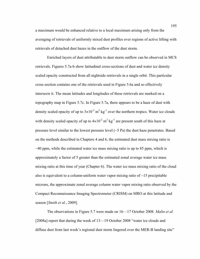
195 a maximum would be enhanced relative to a local maximum arising only from the

averaging of retrievals of uniformly mixed dust profiles over regions of active lifting with

retrievals of detached dust hazes in the outflow of the dust storm.

Enriched layers of dust attributable to dust storm outflow can be observed in MCS

retrievals. Figures 5.7a-b show latitudinal cross-sections of dust and water ice density

scaled opacity constructed from all nightside retrievals in a single orbit. This particular

cross-section contains one of the retrievals used in Figure 5.6a and so effectively

intersects it. The mean latitudes and longitudes of these retrievals are marked on a

topography map in Figure 5.7c. In Figure 5.7a, there appears to be a haze of dust with

density scaled opacity of up to 3×10-3 m2 kg-1 over the northern tropics. Water ice clouds

with density scaled opacity of up to 4×10-2 m2 kg-1 are present south of this haze at

pressure level similar to the lowest pressure level (~5 Pa) the dust haze penetrates. Based

on the methods described in Chapters 4 and 6, the estimated dust mass mixing ratio is

~40 ppm, while the estimated water ice mass mixing ratio is up to 85 ppm, which is

approximately a factor of 5 greater than the estimated zonal average water ice mass

mixing ratio at this time of year (Chapter 6). The water ice mass mixing ratio of the cloud

also is equivalent to a column-uniform water vapor mixing ratio of ~15 precipitable

microns, the approximate zonal average column water vapor mixing ratio observed by the

Compact Reconnaissance Imaging Spectrometer (CRISM) on MRO at this latitude and

season [Smith et al., 2009].

The observations in Figure 5.7 were made on 16—17 October 2008. Malin et al.

[2008a] report that during the week of 13—19 October 2008 “water ice clouds and

diffuse dust from last week’s regional dust storm lingered over the MER-B landing site”

196 at Meridiani Planum. While the observations in Figure 5.7 were made significantly

westward of Meridiani Planum, even higher dust concentrations were present along the

northern tropic further east (Figure 5.6a). (The retrieval at ~10° E in Figure 5.6a does not

have any successful retrievals near it in the same orbit that could confirm directly that

this haze was present over Meridiani Planum.) Malin et al. [2008a] also report dust storm

activity in Chryse Planitia during this week. Since dust concentrations are relatively low

at the longitude of Chryse Planitia (~60° W) in Figure 5.6a, we propose that the dense

dust hazes in Figures 5.6a and 5.7a are the result of advection of dust from “last week’s

regional dust storm” reported by Malin et al. [2008a], which moved from Solis Planum to

Noachis Terra during the previous week [Malin et al., 2008b].

The high density scaled opacities of the water ice clouds that trail the haze are

consistent with this idea. The estimated water vapor equivalent of these clouds is close to

the measured column mixing ratio of water vapor, suggesting that water vapor was very

deeply mixed in the atmosphere, which is a potential result of water vapor being

transported to high altitudes within the advected dust plume.

If the dust haze was advected across the equator, the direction of transport was

opposite to the sense of the modeled mean meridional circulation in northern summer

[e.g., Richardson and Wilson, 2002], in which meridional transport above the surface is

north to south. Therefore, it is possible that the dust was advected in a longitudinally

restricted circulation with flow opposite to the mean meridional circulation. Such a

circulation could be explained by invoking a strong diabatic heat source in the southern

tropics, such as the storm that was the source of the enriched dust layer. In summary,

197 Figure 5.7 seems to show a spectacular example of outflow from a dust storm

producing an apparent maximum in dust mass mixing ratio at high altitude above the

surface.

Dust storm outflow, however, is not a good explanation for the HATDM in late

northern spring and early northern summer, because dust storm activity is relatively rare

in the tropics during this period. Cantor et al. [2001] presents a detailed climatology of

local dust storm activity in 1999. This study lacks coverage in northern spring and early

northern summer, during which the tropical maximum in mass mixing ratio is most

pronounced. But Cantor et al. [2001] does present results from earlier studies using

Viking Orbiter data that are consistent with the presence of very few dust storms in or

near the tropics around the summer solstice. Some local dust storm activity is observed at

around Ls=110° just northwest of Elysium Mons, but activity at other longitudes on the

edge of the northern tropics is relatively rare until northern fall. Cantor et al. [2006]

presents a less detailed but interannual climatology of dust storm activity over most of the

period of Mars Orbiter Camera (MOC) observations and shows that local dust storm

activity around northern summer solstice is generally confined to the polar cap edges,

especially in the northern hemisphere. Therefore, if local dust storms are responsible for

the tropical maximum in mass mixing ratio, only a small number of dust storms could be

involved.

The THEMIS optical depth measurements [Smith, 2009] provide further support

for the absence of dust storms in the tropics. Cap edge dust storm activity in the northern

hemisphere generally has zonal average 1065 cm-1 optical depths of 0.1—0.3. The

tropical dust storm activity in mid to late northern summer of MY 29 is associated with

198 zonal average optical depths of 0.3—0.5 or greater. Zonal average optical depth at

30°-40° N and throughout the tropics is generally 0.05—0.10 through northern spring and

summer, which appears to be too low to indicate dust storm activity.

I also have considered the possibility that outflow from north cap edge dust storm

activity might be advected into the tropics. Such a plume probably would have to cross

the transport barrier due formed by the southerly flow and downwelling due to a

secondary PMOC [Richardson and Wilson, 2002]. This barrier may be manifested by a

region of lower dust density scaled opacity at ~45° N in Figure 5.1a and a mostly

longitudinally uniform band of lower dust concentrations at a similar latitude in Figure

5.2. Moreover, the average dust density scaled opacities around the northern cap edge are

somewhat lower than those observed in the tropics (Figure 5.2), so it seems unlikely that

the northern cap edge activity could be a source of dust for the HATDM.

5.4.3 Orographic Circulations

There are many reasons why high altitude locations on Mars might or might not be

unusually active sites for dust lifting. The main argument against dust lifting at high

altitudes is that the threshold wind velocity for dust lifting is inversely proportional to the

square root of density. This effect may be compensated in part by the higher winds that

generally occur at higher altitudes. In addition, pressures at the high altitudes of Mars are

on the rapidly increasing portion of the Päschen curve of CO2, which may permit stronger

electric fields than at lower altitudes and enhanced dust lifting by electrostatic effects

[Kok and Renno, 2006]. Yet concerns about the difficulty of lifting dust from mountain

tops may be irrelevant to the role of orography in the dust cycle, since mountains on Mars

199 might act as a means for dust to be lifted at lower altitudes but injected into the

atmosphere at higher altitudes.

The proposed dynamics of orographic injection of dust are fairly simple. During

the daytime, the air on the top of the mountain heats more quickly than the air at the

bottom of the mountain due to the lower density of the air at the top of the mountain. In

addition, the air in contact with the surface of the mountain (either summit or slope) is

warmed more quickly than the air at the same altitude away from the mountain. The

heated mountain therefore becomes a local center of low pressure, producing a

convergent anabatic wind that lifts dust from the slopes and makes the air at the top of the

mountain very dusty and even hotter. Simulations by Rafkin et al. [2002] of a cloud and

hypothetically connected orographic thermal circulation on Arsia Mons showed that the

vertical velocities of the anabatic wind were up to 25 ms-1 and needed to be balanced by

extremely strong ( > 40 ms-1) divergent winds at the top of the orographic circulation.

The end result is advection of dust at levels on the order of a few ppm at ~20 km altitude

at a distance up to 2000 km from the mountain. Such a process would be one plausible

source for a HATDM.

The cloud type simulated by Rafkin et al. [2002] is called a “mesoscale spiral

cloud.” This type may be identical to or genetically related to the “aster clouds” observed

by Wang and Ingersoll [2002]. Aster clouds form in late northern summer or early

northern fall, are 200—500 km long, 20—50 km wide, and are found at altitudes of

15 km or more above the surface. Both types of clouds are thought to be generated by

strong upslope winds. As of yet, there is no sufficiently detailed climatology of

mesoscale spiral clouds or aster clouds to permit direct comparison with MCS retrievals.

200 Moreover, the present MCS retrieval dataset is not ideal for isolation of

orographic cloud dynamics for three key reasons. First, the dearth of dayside equatorial

profiles in the tropics throughout much of northern spring and summer limits information

about the aerosol distribution over the volcanoes at the time of day and season when the

upslope winds are thought to be most active. Second, both observations and modeling

[Benson et al., 2006; Michaels et al., 2006] suggest that orographic water ice clouds are

strongly entrained into the global wind field once they escape their local mesoscale

circulations. Orographic dust clouds likely would be subject to the same effect and would

tend to advect zonally. In that case, roughly synchronous (within a few minutes)

observations over the volcano and at adjacent longitudes in the same latitudinal band

could verify their orographic origins. Such observations would be one possible use of

cross-track observations for an instrument on a polar-orbiting spacecraft. Third, if dust

advected from the volcano is blown off at relatively shallow depths above the high

elevation surface, the current retrievals do not reach close enough to the surface to “see”

this dust.

As an example of what is currently possible, Figures 5.8a-e show the seasonal

variability in the vertical dust distribution over Mars’s five tallest volcanoes in order of

increasing latitude (Arsia Mons, Pavonis Mons, Ascraeus Mons, Olympus Mons, and

Elysium Mons) during MY 29. The extrapolated surface pressures of each retrieval are

shown in order to indicate where retrievals are available and show that the profiles are

over relatively high terrain (at least 9 km above the Mars Orbiter Laser Altimeter

(MOLA) datum in all cases). An MCS retrieval, however, is an integration of information

201

Figure 5.8. Log10

of dust density scaled opacity (m2 kg-1) from both dayside and nightside retrievals. The black crosses indicate the Ls and extrapolated surface pressure for each retrieval: (a) near Arsia Mons (7.5°—11.5° S, 115.5°—125.5° W, estimated scene altitude of the profile > 15 km above the MOLA datum); (b) near Pavonis Mons (1.2° S—2.8° N, 108.4°—118.4° W, estimated scene altitude of the profile > 13 km above the MOLA datum); (c) near Ascraeus Mons (9.8°—13.8° N, 99.5°—109.5° W, estimated scene altitude of the profile > 15 km above the MOLA datum); (d) near Olympus Mons (16.4°—20.4° N, 129°—139° W, estimated scene altitude of the profile > 20 km above the MOLA datum); (e) near Elysium Mons (22.8°—26.8° N, 141.9°—151.9° E, estimated scene altitude of the profile > 9 km above the MOLA datum).

202 over a relatively broad volume, so Figures 5.8a-e should not be interpreted as

equivalent to a record of narrow soundings above the volcano’s summit by a balloon or a

lidar.

The atmosphere above the volcanoes is dustier in southern spring and summer

than in northern spring and summer, just like elsewhere in the tropics (Figure 5.1). In

northern spring and summer, the dust distribution over each volcano resembles the dust

distribution at the latitude of the volcano if it were cut off at higher pressures,

followingthe general pattern of the HATDM, which is dustier and present at lower

pressures in the northern tropics than the northern tropics. This contrast can be seen at

~60 Pa during northern spring and much of northern summer. Elysium Mons is much

dustier than Pavonis Mons (Figures 5.8e and 5.8b). Olympus Mons (Figure 5.8d) has a

very high surface, so retrievals do not reach pressures higher than ~40 Pa. In the zonal

average (Figure 5.1), Mars is relatively free of dust at that pressure at this latitude and

season, so Olympus Mons is relatively free of dust. In a few exceptional cases, high dust

density scaled opacities are observed over the volcanoes at ~60 Pa, the approximate

pressure of the HATDM.

Based on the available evidence, orographic injection is not a likely contributor to

the HATDM. If aster clouds are the primary means of dust injection, their climatology (as

presently known) differs from the HATDM. Like tropical dust storm activity, aster clouds

occur too late in northern summer. Moreover, if orographic injection were primarily

responsible for the HATDM, longitudinal inhomogeneities in the dust distribution likely

should take the form of higher dust density scaled opacities downwind and nearer the

volcano than upwind and further away. In Figure 5.3, the cross-sections may sample the

203 modeled and observed path along which water ice clouds over Olympus Mons advect

[Benson et al., 2006; Michaels et al., 2006], which is north and west of Olympus Mons

(134° W). The cross-section likewise intersects Elysium Mons at ~147° E. Yet the

enriched dust layer is of similar density scaled opacity on both sides of Olympus Mons

and indeed density scaled opacity is usually at least half as high around Elysium Mons

than at 60°—120° E. Orographic injection also does not explain the enriched layers of

dust in individuals retrievals at 20°—40° W in Figure 5.2c, a location distant from

significant topography.

Despite poor evidence for the mechanism causing the HATDM, the parsimony of

orographic injection, however, remains attractive. The simplest way of explaining a layer

of dust at 20 km above the mean altitude of the surface is that it comes from a surface 20

km above the mean. As long as the observational record of dust clouds over volcanoes is

sparse and the daytime dust distribution over or near volcanoes remains poorly known, an

orographic source for the HATDM cannot be fully disproven. Past modeling experiments

have focused on the dust transport out of mesoscale circulations around volcanoes. Future

experiments should simulate the contributions of these circulations to the global dust

distribution in greater detail.

5.4.4 Dust Pseudo-Moist Convection

Dust devils are an attractive possible source for the HATDM, since they are thought to be

the dominant mechanism for lifting dust under relatively clear conditions. Fuerstenau

[2006] has proposed that solar heating of the dust load within a dust devil plume could

result in a type of pseudo-moist convection, in which solar heating of the dust load

204 exceeds adiabatic cooling of the parcel. Dust devil plumes therefore might be capable

of breaking through the top of the boundary layer and detraining significant amounts of

dust at altitude.

To supplement simple calculations of Fuerstenau [2006], which neglect the

important process of entrainment of environmental air into dusty parcels, the single

column cloud model of Gregory [2000] was modified to simulate the ascent of dust

parcels. The model of Gregory [2000] has been successful in representing both shallow

and deep cumulus convection on the Earth. In our model, a parcel with a given initial dust

concentration, q0, is in thermal equilibrium with the environment and has some initial

vertical velocity, w0 at the surface (z=0). Kinetic energy is defined as:

€

K =12w2 (5.2)

and the temperature of the parcel is allowed to evolve discretely in the height domain:

€

T(z + Δz) = T(z) − gcpΔz

+

Δzw(z)

εF0 cosξ exp(−τ(z) /cosξ)q(z)cp

ς

(5.3)

where g is the acceleration due to gravity, cp is the heat capacity, Δz is the resolution of

the height grid, ξ is the solar zenith angle, is the efficiency of absorption of solar

radiation by dust (including scattering), F0 is the top of the atmosphere flux, τ is the

environmental optical depth in the solar band, and ς is the conversion factor between

mass mixing ratio and density scaled opacity in the solar band.

The buoyancy is then defined as:

€

B = gTp −TenvTenv

(5.4)

and the entrainment rate, E, is parameterized as:

205

€

E(z + Δz) =ke

w(z)2B(z + Δz)

(5.5)

where ke is a constant. Gregory [2000] estimate the value of this constant to be ~0.045 for

deep cumulus convection and ~0.09 for shallow cumulus convection.

The cooling of the temperature of the parcel and dilution of the dust mass mixing

ratio by entrainment of environmental air is then represented as:

€

Tp* =

EΔzTenv + Tp( )1+ EΔz

,

qp* =

EΔzqenv + qp( )1+ EΔz

(5.6a-b)

if E > 0, where the starred quantities denote the transformed quantities after

entrainment.

Finally, K is allowed to evolve:

€

K(z + Δz) = K(z) + aB(z + Δz) − (2bDK(z)) − (2E(z)K(z))[ ]Δz (5.7)

where a and b are constants derived from large eddy simulations of terrestrial convection,

and are estimated to be 1/6 and 0.5 respectively. D is the detrainment rate, which we

assume to be zero when E > 0 and equal to –E when E < 0. This may be an

underestimate.

The total Convective Available Potential Energy (CAPE) is then estimated as:

€

CAPE = Bdz0

zLNB

∫ (5.8)

where zLNB is the level of neutral buoyancy.

206

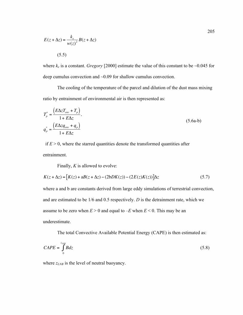
Figure 5.9. Results of simulations of dusty parcels at the Mars Pathfinder site: (a) parcel temperature profile vs. environmental temperature profile; (b) dust mass mixing ratio vs. height; (c) vertical velocity profile of a dusty parcel vs. a dustless parcel; (d) sensitivity of the level of neutral buoyancy to the assumed initial vertical velocity.

207 Table 5.1. Environmental temperature profile used for the single column model simulations of dust-heated convection Height (m) Temperature (K)

0 260

100 251

500 248

1,500 245

10,000 220

20,000 200

30,000 184

40,000 174

50,000 165

208 Table 5.2. Parameters for the single column model simulations of dust-heated convection

Parameter Value Citation (if any)

G 3.73 ms-2 N/A

cp 756 J kg-1 N/A

ς 482 m2 kg-1 N/A

Δz 10 m N/A

ps 670 Pa Schofield et al. [1997]

q0 5*10-3 Metzger et al. [1999]

w0 5 ms-1 N/A

τ0 0.2 N/A

ν 0.1 N/A

ke 0.09 Gregory [2000]

F0 499 Wm-2 N/A

ε 0.11 Tomasko et al. [1999]

ξ 11.8° N/A

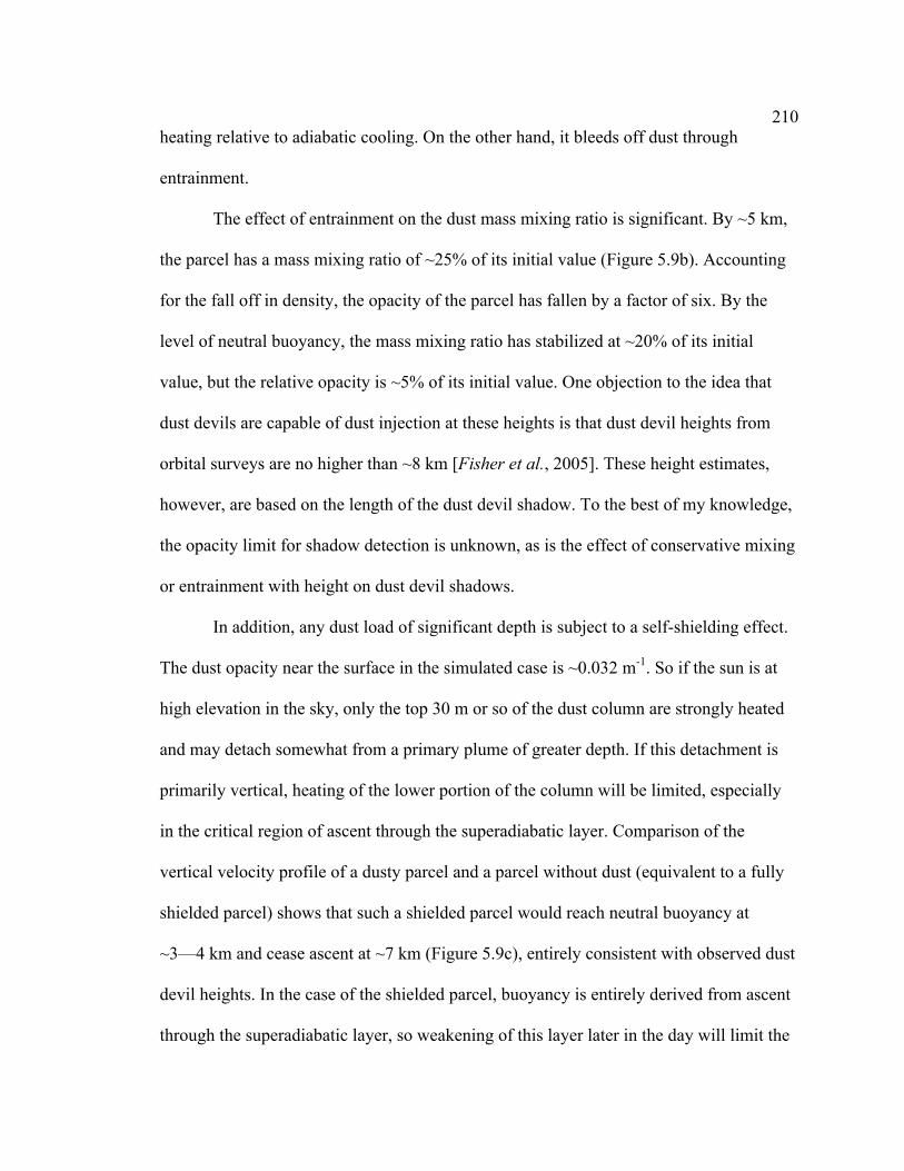
209 Figures 5.9a-d show the results of a single column simulation using Eqs.

5.2—5.8 of hypothetical dust parcels associated with dust devils observed near the Mars

Pathfinder site ~12:40 LST (9:30 UTC) on 15 July 1997 (Ls=148.15°) [Metzger et al.,

1999; Fuerstenau, 2006]. The environmental temperature profile (Table 5.1) is based on

Mars Pathfinder observations, temperature retrievals from the Miniature Thermal

Emission Spectrometer, and Ls=145°—150° zonal average temperatures at the

approximate latitude of Mars Pathfinder during MY 29 from MCS retrievals. The other

parameters of the simulation are given in Table 5.2.

Figure 5.9a shows environmental and parcel temperature profiles of the

simulation: a plot analogous to a SKEW—T diagram used in terrestrial weather

forecasting. Note that the Convective Available Potential Energy (CAPE) of this parcel is

comparable to strong terrestrial thunderstorm activity. The parcel is most strongly heated

within the first couple of kilometers of ascent. Within the same height range,

environmental temperatures decrease quickly in the superadiabatic layer near the strongly

heated surface. At ~1,500 m, the approximate top of the boundary layer in this scenario,

the dusty parcel is almost 20 K warmer than the external environment. The heating effect

from the more dilute dust loading above ~2,500 m is not strong enough to keep the parcel

from cooling more strongly than the environment. This strong gain in buoyancy near the

surface relative to the rest of the path of ascent arises from the assumption that

entrainment is inversely proportional to the square of velocity, so the parcel’s dust

concentration is strongly diluted by entrainment of environmental air when it is moving

more slowly. On one hand, the low vertical velocity of the parcel enhances radiative

210 heating relative to adiabatic cooling. On the other hand, it bleeds off dust through

entrainment.

The effect of entrainment on the dust mass mixing ratio is significant. By ~5 km,

the parcel has a mass mixing ratio of ~25% of its initial value (Figure 5.9b). Accounting

for the fall off in density, the opacity of the parcel has fallen by a factor of six. By the

level of neutral buoyancy, the mass mixing ratio has stabilized at ~20% of its initial

value, but the relative opacity is ~5% of its initial value. One objection to the idea that

dust devils are capable of dust injection at these heights is that dust devil heights from

orbital surveys are no higher than ~8 km [Fisher et al., 2005]. These height estimates,

however, are based on the length of the dust devil shadow. To the best of my knowledge,

the opacity limit for shadow detection is unknown, as is the effect of conservative mixing

or entrainment with height on dust devil shadows.

In addition, any dust load of significant depth is subject to a self-shielding effect.

The dust opacity near the surface in the simulated case is ~0.032 m-1. So if the sun is at

high elevation in the sky, only the top 30 m or so of the dust column are strongly heated

and may detach somewhat from a primary plume of greater depth. If this detachment is

primarily vertical, heating of the lower portion of the column will be limited, especially

in the critical region of ascent through the superadiabatic layer. Comparison of the

vertical velocity profile of a dusty parcel and a parcel without dust (equivalent to a fully

shielded parcel) shows that such a shielded parcel would reach neutral buoyancy at

~3—4 km and cease ascent at ~7 km (Figure 5.9c), entirely consistent with observed dust

devil heights. In the case of the shielded parcel, buoyancy is entirely derived from ascent

through the superadiabatic layer, so weakening of this layer later in the day will limit the

211 ascent of shielded parcels as well. These results suggest that the entire circulation of a

dust devil probably does not penetrate the boundary layer. Instead, a number of small

thermals detached by solar heating from the main dust devil plume ascend and then bring

exceptionally dusty air (800—900 ppm in the simulated case) to 15—25 km altitude.

Figure 5.9d shows the sensitivity of the simulation results to the initial vertical

velocity used and suggests that initial vertical velocities as low as ~2 ms-1 allow parcels

to rise ~10 km. However, if the parcel rises too quickly, solar heating will not be able to

compensate for adiabatic cooling, explaining the decay of the level of neutral buoyancy at

high (and highly unrealistic) initial vertical velocity. In Figure 5.10, the conditions of the

simulation were changed to consider the sensitivity of the results to initial dust mass

mixing ratio of the parcel and initial vertical velocity. The colored contours

conservatively plot the level of neutral buoyancy for each set of assumed conditions. The

white contour marks 4 km, a typical tropical boundary layer height [Hinson et al., 2008],

and envelops a v-shaped phase space, in which the range of initial vertical velocities that

can support boundary-layer breaking convection broadens with increasing initial mass

mixing ratio. At the initial dust mass mixing ratio assumed in the simulation (~5,000

ppm), boundary-layer breaking convection can occur for initial vertical velocities less

than 1 ms-1. Thus, even dust plumes with relatively weak vertical velocities, which might

arise from processes other than dust devils such as local circulations in craters etc., could

be highly unstable with respect to pseudo-moist dust convection.

212

Figure 5.10. Sensitivity of level of neutral buoyancy (m) to initial parcel dust concentration (ppm) and initial parcel vertical velocity (ms-1) The white line indicates the 4,000 m contour, the approximate boundary layer height of the simulation. The white area is indicative of simulations in which the parcel leaves the simulation domain.

213 Using the results from the simulation, the necessary vertical dust mass flux

(

€

ˆ M dust) to produce the HATDM can be estimated as:

€

ˆ M dust =Δpg

qexcess

tsed

(5.9)

where Δp is the pressure thickness of the enriched layer, qexcess is the excess dust mass

mixing ratio of the layer, and tsed is the characteristic time of sedimentation/advection

from the enrichment layer. Assuming Δp=85 Pa, g=3.73 ms-2, qexcess=5×10-6, and tsed of

~106 s, the necessary dust mass flux is: 1.1×10-10 kg m-2 s-1. From this result and the

results of the simulation, the fractional area occupied by these thermals (

€

fthermals) can be

estimated to be:

€

fthermals =ˆ M dust

tthermals

tsol

ρwqthermal

(5.10)

Assuming that the thermals occur only ~10% of the day and w, qthermal, and ρ

correspond to their values at the level of neutral buoyancy of the simulated parcel

(20 ms 1, 9×10-4, and 4×10-3 kg m-3 respectively), the fractional area occupied by thermals

needs only be 1.6×10-5. Estimates of the fractional area occupied by dust devils range

from 2×10-4-6×10-4 [Ferri et al., 2003; Fisher et al., 2005], so the areal footprint of the

thermals can be around an order of magnitude smaller than the areal footprint of dust

devils.

This idea, however, is not observationally falsifiable with the MCS retrieval dataset.

The purported boundary layer breaking dust plumes occur at scales much finer than the

resolution of the observations. Moreover, comparison of dust devil climatologies with

retrieved profiles of dust will not be a sufficiently unambiguous test for two reasons.

214 First, the two most complete surveys of dust devil activity on Mars disagree about

fundamental aspects of the climatology. Cantor et al. [2006] analyze orbital imagery of

dust devils and find that dust devils are far more common in the north than in the south.

Whelley and Greeley [2008] analyzes orbital imagery of dust devil tracks and makes the

opposite conclusion. Second, the sensitivity of pseudo-moist dust convection to

parameters intrinsic to individual plumes such as initial vertical velocity and dust

concentration (Figure 5.10) both raises the possibility that dust sources other than dust

devils may drive pseudo-moist convection and also may introduce difficult to control

intensity related biases in any correlation of dust devil climatologies and the vertical

structure of dust.

Instead, the ease at which this effect can be demonstrated by our model and in the

analysis of Fuerstenau [2006] suggests that this mechanism will become apparent in a

mesoscale or large eddy simulation with rapidly updating radiative transfer. If this

hypothesis is verified, parameterization within a GCM should be possible by upscaling

from the smaller scale simulations. Observational validation likely will require lidar

observations in the tropics in tandem with barometry, thermometry, and anemometry

from a surface weather station.

5.5.5 Scavenging by Water Ice

Following Eq. 5.1, particles settle at a velocity in proportion to their radius. Eq. 5.1 is a

simplification of an approximation of the Cunningham-corrected Stokes velocity at high

Knudsen number (Kn≈60 for a 1 µm particle at the surface of Mars). The full

approximation is:

215

€

vs ≈49ρprgδρvt

(5.11)

where δ is a slip-flow correction parameter and vt is the thermal velocity of the gas

[Murphy et al., 1990]. Condensation of water ice on a dust particle will enhance its

sedimentation velocity by increasing its radius. The new particle, however, will have a

lower density. So if a 1 µm radius dust particle (ρp=3000 kg m-3) grows into a 4 µm

radius ice particle (the approximate reff in the aphelion cloud belt [Clancy et al., 2003]),

ρp of the new particle will be effectively the density of ice (~900 kg m-3). Thus, the

sedimentation velocity will increase by ~20%. If the ice particle is 2 µm in radius with a

1 µm radius core of dust, the sedimentation velocity is reduced by ~5%. Thus, if the ice

particle sizes are close to the average water ice particle size observed from orbit,

condensation of ice on dust does not significantly enhance sedimentation.

Using the Phoenix lidar, Whiteway et al. [2009] observed precipitating ice

particles at ~ 4 km above the surface at night. Based on their sedimentation velocity,

Whiteway et al. [2009] calculates that they could be ellipsoidal particles with a volume

equivalent to a 35 µm radius sphere (or larger if columnar). Ice particles of this size may

nucleate around multiple dust particles and will have sedimentation velocities about an

order of magnitude greater than the sedimentation velocities of 1µm dust particles. If

water ice clouds with particles of similar size to those observed by Whiteway et al. occur

in the tropical atmosphere of Mars below the level of the HATDM, the scavenging of

water ice by dust could create the appearance of a HATDM, subject to the condition that

the vertical dust distribution before interaction with clouds is uniformly mixed to the

altitude of the HATDM and the mass mixing ratio of this distribution is at least as great

216 as the mass mixing ratio of the HATDM. In other words, dust is mixed to the height

of the HATDM during the day and quickly scavenged during the night. In an isothermal

atmosphere, the column opacity (τ) due to such a profile will be:

€

τ = DSOHATDM ρs exp(−z /H)d0

zHATDM

∫ z (5.12)

where zHATDM is the characteristic altitude of the HATDM, DSOHATDM is the

characteristic dust density scaled opacity of the HATDM, and ρs is the air density at the

surface. Eq. 5.12 integrates to:

€

τ = DSOHATDM ρsH 1− exp −zHATDMH

, (5.13)

assuming DSOHATDM=5.5×10-4 m2 kg-1, H=104 m, and zHATDM=2×104 m, τ=0.071. The

visible column opacity corresponding to that column opacity in the A5 channel would be

0.52. Assuming the ratio between opacity in the 1075 cm-1 channel used for dust column

opacity retrieval by THEMIS or TES and visible opacity is ~0.5, the implied column

opacity of the pre-scavenged haze somewhat exceeds retrieved dayside column opacities

at this latitude and season [Smith, 2004; Smith, 2009]. Yet without exact knowledge of

the dust size distribution, converting an opacity in the MCS A5 channel to opacity in any

other region of the spectrum is sufficiently uncertain that the observed dayside column

opacities by TES and THEMIS could be consistent with a hypothetical pre-scavenged

haze.

Another challenge to the possibility of scavenging is that the height of the

HATDM exceeds the observed height of the convective boundary layer [Hinson et al.,

2008] by at least a factor of two. Thus, either the convective boundary layer is deeper

217 than observed, the deep uniform mixing of the pre-scavenged profile is due to some

process other than convective boundary layer overturning, or the pre-scavenged profile is

not uniformly mixed. The first explanation is possible. Hinson et al. [2008] observes the

boundary layer height in the northern tropics before the high altitude tropical maximum

has reached its greatest altitude. Hinson et al. [2008] also observes in late afternoon,

possibly after the boundary layer has reached its greatest depth. The second explanation

is more unlikely. Some alternate form of mixing such as the solar heating of dust would

need to be invoked. Yet such a process likely deepens the planetary boundary layer. The

third explanation would either require a pre-existing vertical dust distribution with a local

maximum in mass mixing ratio high above the surface or result in an unrealistically high

column opacity.

Thus, within the present observational constraints, exceptionally deep dry

boundary layer convection that entrains dust from systems such as dust devils and

uniformly mixes this dust to high altitudes could generate the necessary pre-scavenged

profile. The rarity of high quality dayside MCS retrievals in the tropics during northern

spring and summer does not allow a systematic search for such uniformly mixed profiles.

Yet this idea soon may be testable using column opacity retrievals from nadir and off-

nadir views by MCS. The dayside dust column opacity could be used to simulate (based

on considerations of uniform mixing) a pre-scavenged density scaled opacity limb

profile. If scavenging is a significant process, nightside limb profiles in the vicinity of

dayside dust column opacity measurements will be depleted in dust with respect to the

simulated daytime limb profiles below the altitude of the HATDM.

218 5.5 Summary

The HATDM is a surprising feature of at least the nighttime vertical dust distribution of

Mars for a quarter of its year. While enriched layers of dust at high altitudes above the

surface during the rest of the year may be attributable to dust storms, the HATDM does

not seem to be driven by dust storm activity. Instead, the existence of the HATDM may

be evidence for the significant influence of processes related to topography, boundary

layer circulations, and the water cycle on the global dust distribution during the “clear

season.” Since these processes are physically plausible at other seasons/latitudes, they

may influence the dust distribution during the rest of the year.

219 Bibliography

Balme, M., and R. Greeley (2006), Dust devils on Earth and Mars, Rev. Geophys., 44,

RG3003, doi:10.1029/2005RG000188.

Basu, S., M.I. Richardson, and R.J. Wilson (2004), Simulation of the Martian dust cycle

with the GFDL Mars GCM, J. Geophys. Res., 109, E11006, doi:10.1029/2004JE002243.

Basu, S., J. Wilson, M. Richardson, and A. Ingersoll (2006), Simulation of spontaneous

and variable global dust storms with the GFDL Mars GCM, J. Geophys. Res., 111,

E09004, doi:10.1029/2005JE002660.

Benson, J. L., P.B. James, B.A. Cantor, and R. Remigo (2006), Interannual variability of

water ice clouds over major Martian volcanoes observed by MOC, Icarus, 184, 365–371,

doi:10.1016/j.icarus.2006.03.014.

Cantor, B., M. Malin, and K. S. Edgett (2002), Multiyear Mars Orbiter Camera (MOC)

observations of repeated Martian weather phenomena during the northern summer

season, J. Geophys. Res., 107(E3), 5014, doi:10.1029/2001JE001588.

Cantor, B.A., P.B. James, M. Caplinger, and M.J. Wolff (2001), Martian dust storms:

1999 Mars Orbiter Camera observations, J. Geophys. Res., 106(E10), 23,653–23,687.

Cantor, B. A., K. M. Kanak, and K. S. Edgett (2006), Mars Orbiter Camera observations

of Martian dust devils and their tracks (September 1997 to January 2006) and evaluation

of theoretical vortex models, J. Geophys. Res., 111, E12002, doi:10.1029/2006JE002700.

220 Clancy, R. T., M. J. Wolff, and P. R. Christensen (2003), Mars aerosol studies with

the MGS TES emission phase function observations: Optical depths, particle sizes, and

ice cloud types versus latitude and solar longitude, J. Geophys. Res., 108(E9), 5098,

doi:10.1029/2003JE002058.

Colaprete, A., J. R. Barnes, R. M. Haberle, and F. Montmessin (2008), CO2 clouds,

CAPE and convection on Mars: Observations and general circulation modeling, Planet.

Space Sci., 56(2), 150– 180.

Ferri, F., P. H. Smith, M. Lemmon, and N. O. Rennó (2003), Dust devils as observed by

Mars Pathfinder, J. Geophys. Res., 108(E12), 5133, doi:10.1029/2000JE001421.

Fisher, J. A., M. I. Richardson, C. E. Newman, M. A. Szwast, C. Graf, S. Basu, S. P.

Ewald, A. D. Toigo, and R. J. Wilson (2005), A survey of Martian dust devil activity

using Mars Global Surveyor Mars Orbiter Camera images, J. Geophys. Res., 110,

E03004, doi:10.1029/2003JE002165.

Forget, F., F. Hourdin, R. Fournier, C. Hourdin, O. Talagrand, M. Collins, S.R. Lewis,

P.L. Read and J.-P. Huot (1999), Improved general circulation models of the Martian

atmosphere from the surface to above 80 km, J. Geophys. Res 104, 24155–24175.

Fuerstenau, S. D. (2006), Solar heating of suspended particles and the dynamics of

Martian dust devils, Geophys. Res. Lett., 33, L19S03, doi:10.1029/2006GL026798.

Gregory, D. (2000), Estimation of entrainment rate in simple models of convective

clouds, Q.J.R. Meteorol. Soc, 127(571), 53-72.

221 Haberle, R.M., C.B. Leovy, and J.M. Pollack (1982), Some effects of global dust

storms on the atmospheric circulation of Mars, Icarus, 50, 322-367.

Haberle, R.M., J.B. Pollack, J.R. Barnes, R.W. Zurek, C.B. Leovy, J.R. Murphy, J.

Schaeffer, and H. Lee (1993), Mars atmospheric dynamics as simulated by the

NASA/Ames general circulation model I. The zonal mean circulation, J. Geophys. Res.,

98, 3093-3124.

Hinson, D.P., M. Pätzold, S. Tellmann, B. Häusler, and G.L. Tyler (2008), Depth of the

convective boundary layer on Mars, 198(1), 57-66.

Kahn, R.A., T.Z. Martin, R.W. Zurek, and S.W. Lee (1992), The Martian Dust Cycle in

H.H. Kieffer, B.M. Jakosky, C.W. Snyder, and M.S. Matthews, Mars, 1498 pp.,

University of Arizona Press, Tucson.

Kahre, M. A., J. R. Murphy, R. M. Haberle, F. Montmessin, and J. Schaeffer (2005),

Simulating the Martian dust cycle with a finite surface dust reservoir, Geophys. Res. Lett.,

32, L20204, doi:10.1029/2005GL023495.

Kahre, M. A., J. R. Murphy, and R. M. Haberle (2006), Modeling the Martian dust cycle

and surface dust reservoirs with the NASA Ames general circulation model, J. Geophys.

Res., 111, E06008, doi:10.1029/2005JE002588.

Kahre, M.A., J.L. Hollingsworth, R.M. Haberle, and J.R. Murphy (2008), Investigations

of the variability of dust particle sizes in the martian atmosphere using the NASA Ames

General Circulation Model, Icarus, 195(2), 576-597.

222 Kleinböhl , A., J. T. Schofield, D. M. Kass, W. A. Abdou, C. R. Backus, B. Sen, J. H.

Shirley, W. G. Lawson, M. I. Richardson, F. W. Taylor, N. A. Teanby, and D. J.

McCleese (2009), Mars Climate Sounder limb profile retrieval of atmospheric

temperature, pressure, dust, and water ice opacity, J. Geophys. Res., 114, E10006, doi:

10.1029/2009JE003358.

Kok, J. F., and N. O. Renno (2006), Enhancement of the emission of mineral dust

aerosols by electric forces, Geophys. Res. Lett., 33, L19S10.

Korablev, O. I., V. A. Krasopolsky, A. V. Rodin, and E. Chassefiere (1993), Vertical

structure of the Martian dust measured by the solar infrared occultations from the Phobos

spacecraft, Icarus, 102, 76–87.

Malin, M. C., B. A. Cantor, T.N. Harrison, D.E. Shean and M.R. Kennedy (2008a), MRO

MARCI Weather Report for the week of 13 October 2008 – 19 October 2008, Malin

Space Science Systems Captioned Image Release, MSSS-55,

http://www.msss.com/msss_images/2008/10/22/.

Malin, M. C., B. A. Cantor, T.N. Harrison, D.E. Shean and M.R. Kennedy (2008b), MRO

MARCI Weather Report for the week of 6 October 2008 – 12 October 2008, Malin Space

Science Systems Captioned Image Release, MSSS-54,

http://www.msss.com/msss_images/2008/10/15/.

McCleese, D. J., J. T. Schofield, F. W. Taylor, S. B. Calcutt, M. C. Foote, D. M. Kass, C.

B. Leovy, D. A. Paige, P. L. Read, and R. W. Zurek (2007), Mars Climate Sounder: An

223 investigation of thermal and water vapor structure, dust and condensate distributions

in the atmosphere, and energy balance of the polar regions, J. Geophys. Res., 112,

E05S06, doi:10.1029/2006JE002790.

McCleese, D.J., J.T. Schofield, F.W. Taylor, W.A. Abdou, O. Aharonson, D. Banfield,

S.B. Calcutt, N.G. Heavens, P.G.J. Irwin, D.M. Kass, A. Kleinböhl, W.G. Lawson, C.B.

Leovy, S.R. Lewis, D.A. Paige, P.L. Read, M.I. Richardson, N. Teanby, and R.W. Zurek

(2008), Nature Geosci., 1, 745-749, doi:10.1038/ngeo332.

Metzger, S. M., J. R. Carr, J. R. Johnson, T. J. Parker, and M. T. Lemmon (1999), Dust

devil vortices seen by the Mars Pathfinder Camera, Geophys. Res. Lett., 26(18), 2781–

2784.

Michaels, T.I., A. Colaprete, and S. C. R. Rafkin (2006), Significant vertical water

transport by mountain‐induced circulations on Mars, Geophys. Res. Lett., 33, L16201,

doi:10.1029/2006GL026562.

Murphy, J. R., O. B. Toon, R. M. Haberle, and J. B. Pollack (1990), Numerical

Simulations of the Decay of Martian Global Dust Storms, J. Geophys. Res., 95(B9),

14,629–14,648.

Newman, C. E., S. R. Lewis, P. L. Read, and F. Forget (2002a), Modeling the Martian

dust cycle, 1. Representations of dust transport processes, J. Geophys. Res., 107(E12),

5123, doi:10.1029/2002JE001910.

224 Newman, C. E., S. R. Lewis, P. L. Read, and F. Forget (2002b), Modeling the

Martian dust cycle 2. Multiannual radiatively active dust transport simulations, J.

Geophys. Res., 107(E12), 5124, doi:10.1029/2002JE001920.

Putzig, N. E., M. T. Mellon, K. A. Kretke, and R. E. Arvidson (2005), Global thermal

inertia and surface properties of Mars from the MGS mapping mission, Icarus 173, 325-

341.

Rafkin, S. C. R., M. R. V. Sta. Maria, and T. I. Michaels (2002), Simulation of the

atmospheric thermal circulation of a martian volcano using a mesoscale numerical model.

Nature, 419, 697-699.

Richardson, M.I. and R.J. Wilson (2002), A topographically forced asymmetry in the

martian circulation and climate. Nature 416 (6878), 298-301.

Schneider, E.K. (1983), Martian Great Dust Storms: Interpretive Axially Symmetric

Models, Icarus, 35, 302-331.

Schofield, J. T., J. R. Barnes, D. Crisp, R. M. Haberle, S. Larsen, J. A. Magalhães, J. R.

Murphy, A. Seiff, and G. Wilson (1997), The Mars Pathfinder Atmospheric Structure

Investigation/Meteorology (ASI/MET) Experiment, Science, 278, 1752–1758.

Smith, M. D. (2004), Interannual variability in TES atmospheric observations of Mars

during 1999– 2003, Icarus, 108, 148– 165.

225 Smith, M.D. (2009), THEMIS Observations of Mars aerosol optical depth from

2002—2008, Icarus, 202 (2), 444-452, doi:10.1016/j.icarus.2009.03.027.

Smith, M. D., M. J. Wolff, R. T. Clancy, and S. L. Murchie (2009), Compact

Reconnaissance Imaging Spectrometer observations of water vapor and carbon

monoxide, J. Geophys. Res., 114, E00D03, doi:10.1029/2008JE003288.

Strausberg, M. J., H. Wang, M. I. Richardson, S. P. Ewald, and A. D. Toigo (2005),

Observations of the initiation and evolution of the 2001 Mars global dust storm, J.

Geophys. Res., 110, E02006, doi:10.1029/2004JE002361.

Szwast, M. A., M. I. Richardson, and A. R. Vasavada (2006), Surface dust redistribution

on Mars as observed by the Mars Global Surveyor and Viking orbiters, J. Geophys. Res.,

111, E11008, doi:10.1029/2005JE002485.

Thomas, P. and P.J. Gierasch (1985), Dust Devils on Mars, Science, 230 (4722), 175-177.

Tomasko, M. G., L. R. Doose, M. Lemmon, P. H. Smith, and E. Wegryn (1999),

Properties of dust in the Martian atmosphere from the Imager on Mars Pathfinder, J.

Geophys. Res., 104(E4), 8987–9007.

Wang, H., and A. P. Ingersoll (2002), Martian clouds observed by Mars Global Surveyor

Mars Orbiter Camera, J. Geophys. Res., 107(E10), 5078, doi:10.1029/2001JE001815.

Whelley, P. L., and R. Greeley (2008), The distribution of dust devil activity on Mars, J.

Geophys. Res., 113, E07002, doi:10.1029/2007JE002966.

226 Whiteway, J. A., Komguem, L., Dickinson, C., Cook, C., Illnicki, M., Seabrook, J.,

Popovici, V., Duck, T. J., Davy, R., Taylor, P. A., Pathak, J., Fisher, D., Carswell, A. I.,

Daly, M., Hipkin, V., Zent, A. P., Hecht, M. H., Wood, S. E., Tamppari, L. K., Renno,

N., Moores, J. E., Lemmon, M. T., Daerden, F., Smith, P. H. (2009) Mars Water-Ice

Clouds and Precipitation, Science, 325 (5936), 68-70. doi: 10.1126/science.1172344.

Zurek, R.W., J.R. Barnes, R.M. Haberle, J.B. Pollack, J.E. Tillman, and C.B. Leovy

(1992), Dynamics of the Atmosphere of Mars in H.H. Kieffer, B.M. Jakosky, C.W.

Snyder, and M.S. Matthews, Mars, 1498 pp., University of Arizona Press, Tucson.