chapter 5. stress-strain relationships and behavior

Seoul National University

Mechanical Strengths and Behavior of Solids

2015/8/9 - 1 -

Chapter 5. Stress-Strain Relationships and Behavior


Contents

2015/8/9 - 2 -

1 Introduction

2 Models for Deformation Behavior

3 Elastic Deformation

4 Anisotropic Materials


5.1 Introduction

2015/8/9 - 3 -

• Three major types of deformation: Elastic, Plastic, and Creep deformation

• In engineering analysis, constitutive equations which describe stress-strain relationships are essential to calculate stresses and deflections in mechanical components.

• Consider one-dimensional stress-strain behavior and some corresponding simple physical models for each deformation.

• Three-dimensional elastic deformation: Isotropy and Anisotropy– Isotropy: The elastic properties are the same in all directions.– Anisotropy: The elastic properties vary with direction.


5.2 Models for Deformation Behavior

2015/8/9 - 4 -

Figure 5.1 Mechanical models for four types of deformation. The displacement–time and force–displacement responses are also shown for step inputs of force P, which is analogous to stress σ. Displacement x is analogous to strain ε.

𝜂𝜂 : coefficient of tensile viscosity(in analogous to c)


Plastic Deformation Models (1)

2015/8/9 - 5 -

Figure 5.3 Rheological models for plastic deformation and their responses to three different strain inputs. Model (a) has behavior that is rigid, perfectly plastic; (b) elastic, perfectly plastic; and (c) elastic, linear hardening.

𝐸𝐸1𝐸𝐸2𝐸𝐸1 + 𝐸𝐸2


Plastic Deformation Models (2)

2015/8/9 - 6 -

• The point during unloading where the stress passes through zero‒ Elastic unloading of the same slope 𝐸𝐸1 as the initial loading‒ The elastic strain 𝜀𝜀𝑒𝑒 is recovered corresponds to the relaxation of spring 𝐸𝐸1.‒ The permanent or plastic strain 𝜀𝜀𝑝𝑝 corresponds to the motion of the slider

up to the point of maximum strain.

Figure 5.4 Loading and unloading behavior of (a) an elastic, perfectly plastic model, (b) an elastic, linear-hardening model, and (c) a material with nonlinear hardening.


Creep Deformation Models (1)

2015/8/9 - 7 -

Figure 5.5 Rheological models having time-dependent behavior and their responses to a stress–time step. Both strain–time and stress–strain responses are shown. Model (a) exhibits steady-state creep with elastic strain added, and model (b) transient creep with elastic strain added.

Spring: 𝜀𝜀𝑒𝑒 = 𝜎𝜎′

𝐸𝐸1

Dashpot: 𝜀𝜀𝑐𝑐 = 𝜎𝜎′

𝜂𝜂1

Linear viscoelasticity Some polymers, ceramics, and metals at high temperature, but low stress

Nonlinear viscoelasticityMetals and ceramics at high stress


Creep Deformation Models (2)

2015/8/9 - 8 -

• For the steady-state creep model of Fig. 5.5(a),𝜀𝜀 = 𝜀𝜀𝑒𝑒 + 𝜀𝜀𝑐𝑐 =

𝜎𝜎′

𝐸𝐸1+ 𝜀𝜀𝑐𝑐

The rate of creep strain: 𝜀𝜀𝑐𝑐 = 𝑑𝑑𝜀𝜀𝑐𝑐𝑑𝑑𝑑𝑑

= 𝜎𝜎′

𝜂𝜂1

Solving 𝜀𝜀𝑐𝑐 by integration, 𝜀𝜀 = 𝜎𝜎′

𝐸𝐸1+ 𝜎𝜎′𝑑𝑑

𝜂𝜂1 After removal of the stress, elastic strain disappears, but the creep strain accumulated during 1-2 remains as a permanent strain.

• For the transient creep model of Fig. 5.5(b),The stress in the (𝜂𝜂2,𝐸𝐸2) stage:

𝜎𝜎 = 𝐸𝐸2𝜀𝜀2 + 𝜂𝜂2 𝜀𝜀𝑐𝑐This gives

𝜀𝜀𝑐𝑐 =𝑑𝑑𝜀𝜀𝑐𝑐𝑑𝑑𝑑𝑑 =

𝜎𝜎 − 𝐸𝐸2𝜀𝜀𝑐𝑐𝜂𝜂2

Solving this differential equation,

𝜀𝜀 =𝜎𝜎′

𝐸𝐸1+𝜎𝜎′

𝐸𝐸2(1 − 𝑒𝑒−

𝐸𝐸2𝑑𝑑𝜂𝜂2 )

Strain rate decreases with time and creep strain asymptotically approaches the limit ⁄𝜎𝜎′ 𝐸𝐸2. After stress removal, the transient creep strain decreases toward zero at infinite time due to the spring. The equation for the recovery response can be obtained by solving ODE.


Relaxation Behavior (1) (optional)

2015/8/9 - 9 -

• Creep: Accumulation of strain with time, as under constant stress• Recovery: Gradual disappearance of creep strain that occurs after

removal of the stress• Relaxation: Decrease in stress when a material is held at constant strain

Figure 5.7 Stress–time step applied to a material exhibiting strain response that includes elastic, plastic, and creep components.

Relaxation



2015/8/9 - 10 -

• Creep: Accumulation of strain with time, as under constant stress• Recovery: Gradual disappearance of creep strain that occurs after

removal of the stress• Relaxation: Decrease in stress when a material is held at constant strain

Figure 5.6 Relaxation under constant strain for a model with steady-state creep and elastic behavior. The step in strain (a) causes stress–time behavior as in (b), and stress–strain behavior as in (c).

Relaxation



2015/8/9 - 11 -

• About sudden strain 𝜀𝜀′, it is absorbed by the spring entirely because the dashpot requires a finite time to respond.

• Due to the total strain being held constant, the strain in the spring decreases, as the strain in the dashpot increases.

𝜀𝜀′ = 𝜀𝜀𝑒𝑒 + 𝜀𝜀𝑐𝑐 = 𝑐𝑐𝑐𝑐𝑐𝑐𝑐𝑐𝑑𝑑.

The stress necessary to maintain the constant strain:𝜎𝜎 = 𝐸𝐸1𝜀𝜀𝑒𝑒

The rate of creep strain:

𝜀𝜀𝑐𝑐 =𝑑𝑑𝜀𝜀𝑐𝑐𝑑𝑑𝑑𝑑

=𝜎𝜎𝜂𝜂1

Combining these equations and solving the differential equation:

𝜎𝜎 = 𝐸𝐸1𝜀𝜀′𝑒𝑒−𝐸𝐸1𝑑𝑑𝜂𝜂1

• If the strain is returned to zero, the stress is forced into compression. Additional relaxation the occurs, but in the opposite direction, as the relaxation always proceeds toward zero stress.


5.3 Elastic Deformation

2015/8/9 - 12 -


Elastic Constants (1)

2015/8/9 - 13 -

• Homogeneous: A material that has the same properties at all points within the solid

• Isotropic: A material whose properties are the same in all directions

Figure 5.8 Longitudinal extension and lateral contraction used to obtain constants for a linear-elastic material that is isotropic and homogeneous.

‒ Elastic modulus𝐸𝐸 =

𝜎𝜎𝑥𝑥𝜀𝜀𝑥𝑥

‒ Poisson’s ratio

𝜈𝜈 = −𝑑𝑑𝑡𝑡𝑡𝑡𝑐𝑐𝑐𝑐𝑡𝑡𝑒𝑒𝑡𝑡𝑐𝑐𝑒𝑒 𝑐𝑐𝑑𝑑𝑡𝑡𝑡𝑡𝑠𝑠𝑐𝑐𝑙𝑙𝑐𝑐𝑐𝑐𝑙𝑙𝑠𝑠𝑑𝑑𝑙𝑙𝑑𝑑𝑠𝑠𝑐𝑐𝑡𝑡𝑙𝑙 𝑐𝑐𝑑𝑑𝑡𝑡𝑡𝑡𝑠𝑠𝑐𝑐

= −𝜀𝜀𝑦𝑦𝜀𝜀𝑥𝑥

‒ From elastic modulus and Poisson’s ratio

𝜀𝜀𝑦𝑦 = −𝜈𝜈𝐸𝐸𝜎𝜎𝑥𝑥


Elastic Constants (2)

2015/8/9 - 14 -

• Poisson’s ratio is often around 0.3, 0 < 𝜈𝜈 < 0.5.

• Negative values of 𝜈𝜈 imply lateral expansion during axial tension.

• 𝜈𝜈 = 0.5 implies constant volume, and values lager than 0.5 imply a decrease in volume for tensile loading.

• Small-strain theory: When dimensional changes are small, original dimensions and cross-sectional areas are used to determine stresses and strains.

• If a given metal is alloyed with small percentages of other metals, the elastic constants 𝐸𝐸 and 𝜈𝜈 can be approximated as being the same as the corresponding pure metal values.‒ Aluminum and titanium alloys: less than 10%‒ Low-alloy steels: less than 5%


Hooke’s Law for Three Dimensions (1)

2015/8/9 - 15 -

Figure 5.9 The six components needed to completely describe the state of stress at a point.

Resulting Strain Each Direction

Stress X Y Z

𝜎𝜎𝑥𝑥 𝜎𝜎𝑥𝑥𝐸𝐸

−𝜈𝜈𝜎𝜎𝑥𝑥𝐸𝐸

−𝜈𝜈𝜎𝜎𝑥𝑥𝐸𝐸

𝜎𝜎𝑦𝑦 −𝜈𝜈𝜎𝜎𝑦𝑦𝐸𝐸

𝜎𝜎𝑦𝑦𝐸𝐸

−𝜈𝜈𝜎𝜎𝑦𝑦𝐸𝐸

𝜎𝜎𝑧𝑧 −𝜈𝜈𝜎𝜎𝑧𝑧𝐸𝐸

−𝜈𝜈𝜎𝜎𝑧𝑧𝐸𝐸

𝜎𝜎𝑧𝑧𝐸𝐸

𝜀𝜀𝑥𝑥 =1𝐸𝐸𝜎𝜎𝑥𝑥 − 𝜈𝜈 𝜎𝜎𝑦𝑦 + 𝜎𝜎𝑧𝑧

𝜀𝜀𝑦𝑦 =1𝐸𝐸

[𝜎𝜎𝑦𝑦 − 𝜈𝜈 𝜎𝜎𝑥𝑥 + 𝜎𝜎𝑧𝑧 ]

𝜀𝜀𝑧𝑧 =1𝐸𝐸

[𝜎𝜎𝑧𝑧 − 𝜈𝜈 𝜎𝜎𝑥𝑥 + 𝜎𝜎𝑦𝑦 ]

The strains caused by stresses in each direction: Total strain in each direction:

• Three normal stresses:𝜎𝜎𝑥𝑥,𝜎𝜎𝑦𝑦 , and 𝜎𝜎𝑧𝑧

• Three shear stresses:𝜏𝜏𝑥𝑥𝑦𝑦 , 𝜏𝜏𝑦𝑦𝑧𝑧, and 𝜏𝜏𝑧𝑧𝑥𝑥


Hooke’s Law for Three Dimensions (2)

2015/8/9 - 16 -

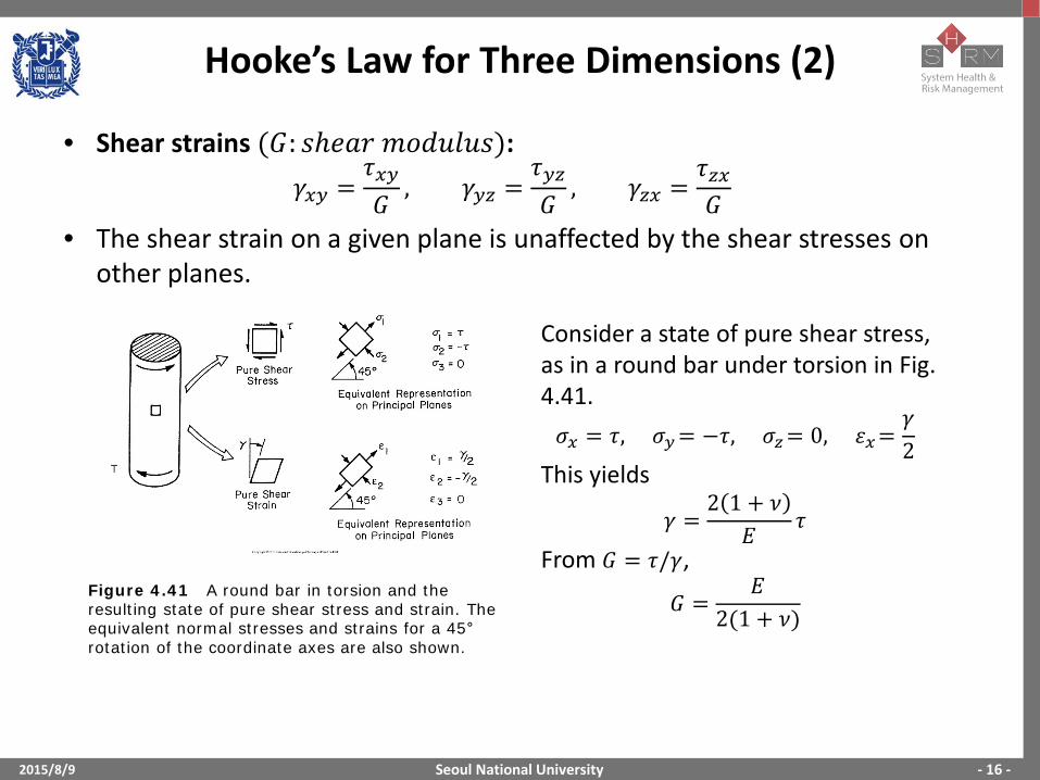
• Shear strains (𝐺𝐺: 𝑐𝑐𝑠𝑒𝑒𝑡𝑡𝑡𝑡 𝑚𝑚𝑐𝑐𝑑𝑑𝑙𝑙𝑙𝑙𝑙𝑙𝑐𝑐):𝛾𝛾𝑥𝑥𝑦𝑦 =

𝜏𝜏𝑥𝑥𝑦𝑦𝐺𝐺

, 𝛾𝛾𝑦𝑦𝑧𝑧 =𝜏𝜏𝑦𝑦𝑧𝑧𝐺𝐺

, 𝛾𝛾𝑧𝑧𝑥𝑥 =𝜏𝜏𝑧𝑧𝑥𝑥𝐺𝐺

• The shear strain on a given plane is unaffected by the shear stresses on other planes.

Figure 4.41 A round bar in torsion and the resulting state of pure shear stress and strain. The equivalent normal stresses and strains for a 45°rotation of the coordinate axes are also shown.

Consider a state of pure shear stress, as in a round bar under torsion in Fig. 4.41.𝜎𝜎𝑥𝑥 = 𝜏𝜏, 𝜎𝜎𝑦𝑦= −𝜏𝜏, 𝜎𝜎𝑧𝑧= 0, 𝜀𝜀𝑥𝑥=

𝛾𝛾2

This yields

𝛾𝛾 =2 1 + 𝜈𝜈

𝐸𝐸𝜏𝜏

From 𝐺𝐺 = 𝜏𝜏/𝛾𝛾,

𝐺𝐺 =𝐸𝐸

2(1 + 𝜈𝜈)


Volumetric Strain

2015/8/9 - 17 -

The normal strains:

𝜀𝜀𝑥𝑥 =𝑑𝑑𝑑𝑑𝑑𝑑

, 𝜀𝜀𝑦𝑦 =𝑑𝑑𝑑𝑑𝑑𝑑

, 𝜀𝜀𝑧𝑧 =𝑑𝑑𝑑𝑑𝑑𝑑

From 𝑉𝑉 = 𝑑𝑑𝑑𝑑𝑑𝑑,

𝑑𝑑𝑉𝑉 =𝜕𝜕𝑉𝑉𝜕𝜕𝑑𝑑

𝑑𝑑𝑑𝑑 +𝜕𝜕𝑉𝑉𝜕𝜕𝑑𝑑

𝑑𝑑𝑑𝑑 +𝜕𝜕𝑉𝑉𝜕𝜕𝑑𝑑

𝑑𝑑𝑑𝑑

Evaluating the partial derivatives and dividing both sides by 𝑉𝑉 = 𝑑𝑑𝑑𝑑𝑑𝑑,

𝑑𝑑𝑉𝑉𝑉𝑉

=𝑑𝑑𝑑𝑑𝑑𝑑

+𝑑𝑑𝑑𝑑𝑑𝑑

+𝑑𝑑𝑑𝑑𝑑𝑑

Figure 5.10 Volume change due to normal strains.

Volumetric strain or dilatation, 𝜀𝜀𝑣𝑣: Ratio of the change in volume

𝜀𝜀𝑣𝑣 =𝑑𝑑𝑉𝑉𝑉𝑉

= 𝜀𝜀𝑥𝑥 + 𝜀𝜀𝑦𝑦 + 𝜀𝜀𝑧𝑧

For an isotropic material (by Hooke’s law),

𝜀𝜀𝑣𝑣 =1 − 2𝜈𝜈𝐸𝐸

(𝜎𝜎𝑥𝑥 + 𝜎𝜎𝑦𝑦 + 𝜎𝜎𝑧𝑧)


Hydrostatic Stress

2015/8/9 - 18 -

• Hydrostatic stress: The average normal stress𝜎𝜎ℎ =

𝜎𝜎𝑥𝑥 + 𝜎𝜎𝑦𝑦 + 𝜎𝜎𝑧𝑧3

Substituting this into volumetric strain for an isotropic material,

𝜀𝜀𝑣𝑣 =3 1 − 2𝜈𝜈

𝐸𝐸𝜎𝜎ℎ

• Bulk modulus: The constant of proportionality between volumetric strain and hydrostatic stress

𝐵𝐵 =𝜎𝜎ℎ𝜀𝜀𝑣𝑣

=𝐸𝐸

3 1 − 2𝜈𝜈

• 𝜀𝜀𝑣𝑣 and 𝜎𝜎ℎ are invariant quantities which always have the same values, regardless of the choice of coordinate system.

• In other words, the sum of the normal strains and the sum of the normal stresses will have the same value for any coordinate system.


Thermal Strains

2015/8/9 - 19 -

• Thermal Strain: Elastic strain caused by the temperature changes𝜀𝜀 = 𝛼𝛼 𝑇𝑇 − 𝑇𝑇0 = 𝛼𝛼(∆𝑇𝑇)

Figure 5.11 Force vs. distance between atoms. A thermal oscillation of equal potential energies about the equilibrium position xe gives an average distance xavg greater than xe.

Figure 5.12 Coefficients of thermal expansion at room temperature versus melting temperature for various materials. (Data from [Boyer 85] p. 1.44, [Creyke 82] p. 50, and [ASM 88] p. 69.)


5.4 Anisotropic Materials

2015/8/9 - 20 -

Figure 5.14 Anisotropic materials: (a) metal plate with oriented grain structure due to rolling, (b) wood, (c) glass-fiber cloth in an epoxy matrix, and (d) a single crystal.


Anisotropic Hooke’s Law

2015/8/9 - 21 -

• The general anisotropic form of Hooke’s law:𝜀𝜀𝑥𝑥𝜀𝜀𝑦𝑦𝜀𝜀𝑧𝑧𝛾𝛾𝑦𝑦𝑧𝑧𝛾𝛾𝑧𝑧𝑥𝑥𝛾𝛾𝑥𝑥𝑦𝑦

=𝑆𝑆11 ⋯ 𝑆𝑆16⋮ ⋱ ⋮𝑆𝑆16 ⋯ 𝑆𝑆66

𝜎𝜎𝑥𝑥𝜎𝜎𝑦𝑦𝜎𝜎𝑧𝑧𝜏𝜏𝑦𝑦𝑧𝑧𝜏𝜏𝑧𝑧𝑥𝑥𝜏𝜏𝑥𝑥𝑦𝑦

• 𝑆𝑆𝑖𝑖𝑖𝑖 change if the orientation of the x-y-z coordinate system is changed.• Each unique 𝑆𝑆𝑖𝑖𝑖𝑖 has a different nonzero value.• The matrix is symmetrical with 21 independent variables.• In the isotropic case,

𝑆𝑆𝑖𝑖𝑖𝑖 =

1/𝐸𝐸 −𝜈𝜈/𝐸𝐸 −𝜈𝜈/𝐸𝐸−𝜈𝜈/𝐸𝐸 1/𝐸𝐸 −𝜈𝜈/𝐸𝐸−𝜈𝜈/𝐸𝐸 −𝜈𝜈/𝐸𝐸 1/𝐸𝐸

0

01/𝐺𝐺 0 0

0 1/𝐺𝐺 00 0 1/𝐺𝐺


Orthotropic Materials; Other Special Cases

2015/8/9 - 22 -

• Orthotropic material: The material that possesses symmetry about three orthogonal planes‒ The coefficients for Hooke’s law for an orthotropic material:

𝑆𝑆𝑖𝑖𝑖𝑖 =

1/𝐸𝐸𝑋𝑋 −𝜈𝜈𝑌𝑌𝑋𝑋/𝐸𝐸𝑌𝑌 −𝜈𝜈𝑍𝑍𝑋𝑋/𝐸𝐸𝑍𝑍−𝜈𝜈𝑋𝑋𝑌𝑌/𝐸𝐸𝑋𝑋 1/𝐸𝐸𝑌𝑌 −𝜈𝜈𝑍𝑍𝑌𝑌/𝐸𝐸𝑍𝑍−𝜈𝜈𝑋𝑋𝑍𝑍/𝐸𝐸𝑋𝑋 −𝜈𝜈𝑌𝑌𝑍𝑍/𝐸𝐸𝑌𝑌 1/𝐸𝐸𝑍𝑍

0

01/𝐺𝐺𝑌𝑌𝑍𝑍 0 0

0 1/𝐺𝐺𝑍𝑍𝑋𝑋 00 0 1/𝐺𝐺𝑋𝑋𝑌𝑌

• Cubic material: The material that has the same properties in the X-, Y-, and Z-directions‒ Three independent constants: 𝐸𝐸𝑋𝑋,𝐺𝐺𝑋𝑋𝑌𝑌, 𝜈𝜈𝑋𝑋𝑌𝑌‒ There is still one more independent constant than for the isotropic case, and

the elastic constants still apply only for the special X-Y-Z coordination system.• Transversely isotropic material: The properties are the same all

directions in a plane, such as the X-Y plane‒ Five independent constants: 𝐸𝐸𝑋𝑋, 𝜈𝜈𝑋𝑋𝑌𝑌,𝐸𝐸𝑍𝑍, 𝜈𝜈𝑋𝑋𝑍𝑍,𝐺𝐺𝑋𝑋𝑍𝑍


Orthotropic Materials

2015/8/9 - 23 -

Orthogonal planes of symmetry

Orthotropic material Transversely isotropic material


Fibrous Composites

2015/8/9 - 24 -

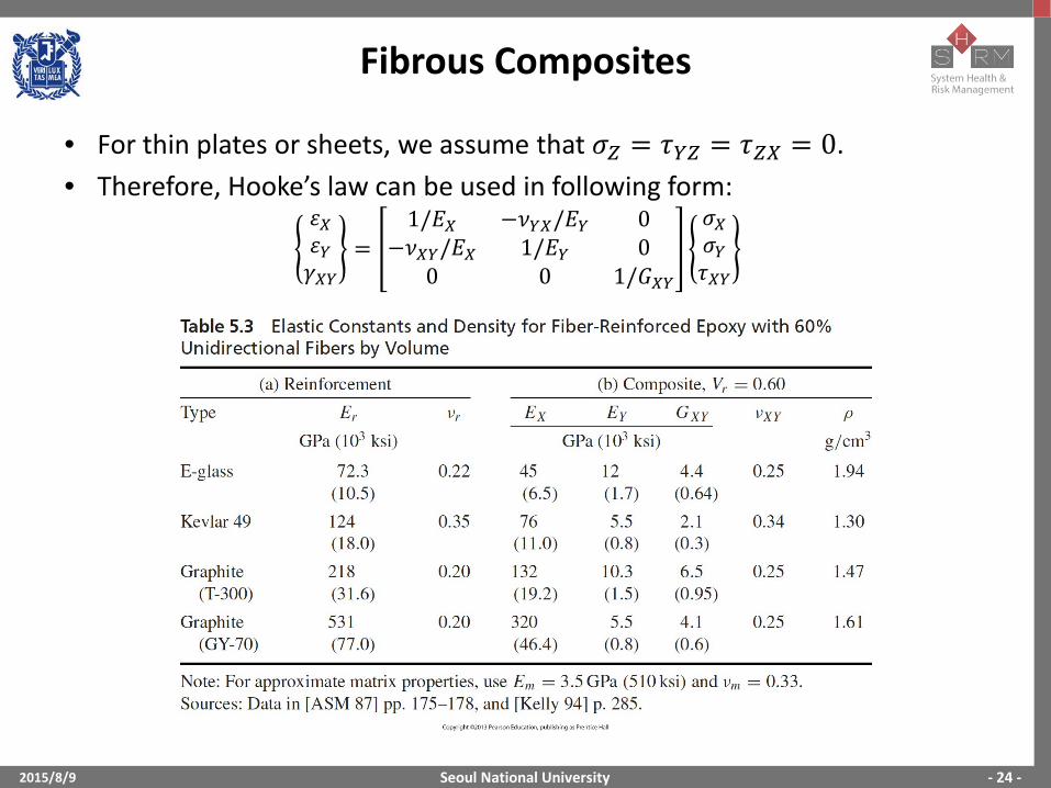
• For thin plates or sheets, we assume that 𝜎𝜎𝑍𝑍 = 𝜏𝜏𝑌𝑌𝑍𝑍 = 𝜏𝜏𝑍𝑍𝑋𝑋 = 0.• Therefore, Hooke’s law can be used in following form:

𝜀𝜀𝑋𝑋𝜀𝜀𝑌𝑌𝛾𝛾𝑋𝑋𝑌𝑌

=1/𝐸𝐸𝑋𝑋 −𝜈𝜈𝑌𝑌𝑋𝑋/𝐸𝐸𝑌𝑌 0

−𝜈𝜈𝑋𝑋𝑌𝑌/𝐸𝐸𝑋𝑋 1/𝐸𝐸𝑌𝑌 00 0 1/𝐺𝐺𝑋𝑋𝑌𝑌

𝜎𝜎𝑋𝑋𝜎𝜎𝑌𝑌𝜏𝜏𝑋𝑋𝑌𝑌


Elastic Modulus Parallel to Fibers (1)

2015/8/9 - 25 -

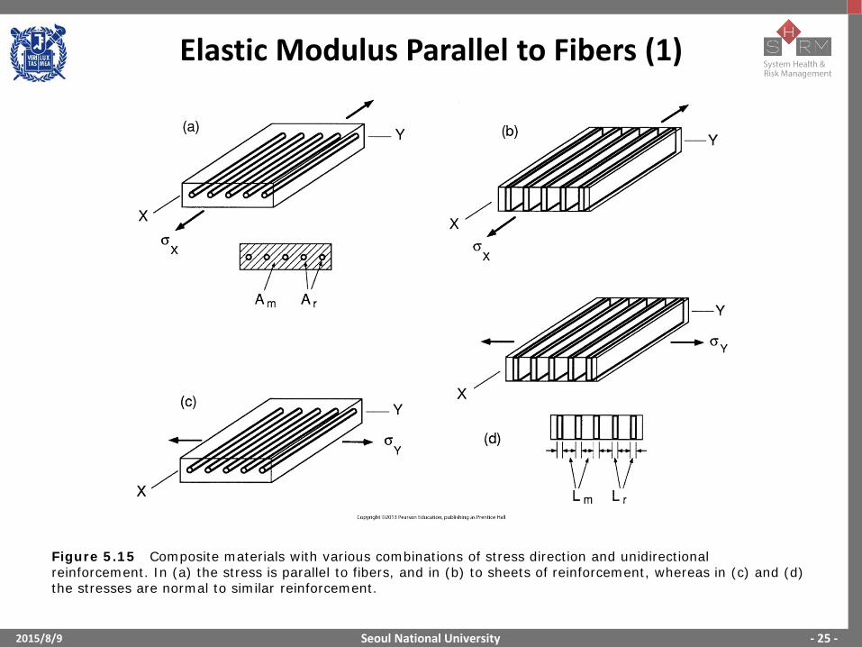
Figure 5.15 Composite materials with various combinations of stress direction and unidirectional reinforcement. In (a) the stress is parallel to fibers, and in (b) to sheets of reinforcement, whereas in (c) and (d) the stresses are normal to similar reinforcement.


Elastic Modulus Parallel to Fibers (2)

2015/8/9 - 26 -

• Fibers: isotropic material with elastic constant 𝐸𝐸𝑟𝑟 , 𝜈𝜈𝑟𝑟, and 𝐺𝐺𝑟𝑟• Matrix: isotropic material with elastic constant 𝐸𝐸𝑚𝑚, 𝜈𝜈𝑚𝑚, and 𝐺𝐺𝑚𝑚• Consider a uniaxial stress 𝜎𝜎𝑋𝑋 parallel to fibers.• Assumption: The fibers are perfectly bonded to the matrix.

𝐴𝐴 = 𝐴𝐴𝑟𝑟 + 𝐴𝐴𝑚𝑚𝜎𝜎𝑋𝑋𝐴𝐴 = 𝜎𝜎𝑟𝑟𝐴𝐴𝑟𝑟 + 𝜎𝜎𝑚𝑚𝐴𝐴𝑚𝑚

𝜎𝜎𝑋𝑋 = 𝐸𝐸𝑋𝑋𝜀𝜀𝑋𝑋, 𝜎𝜎𝑟𝑟 = 𝐸𝐸𝑟𝑟𝜀𝜀𝑟𝑟 , 𝜎𝜎𝑚𝑚 = 𝐸𝐸𝑚𝑚𝜀𝜀𝑚𝑚

From the assumption (𝜀𝜀𝑋𝑋 = 𝜀𝜀𝑟𝑟 = 𝜀𝜀𝑚𝑚), yielding the modulus of the composite material:

𝐸𝐸𝑋𝑋 =𝐸𝐸𝑟𝑟𝐴𝐴𝑟𝑟 + 𝐸𝐸𝑚𝑚𝐴𝐴𝑚𝑚

𝐴𝐴Volume fractions:

𝑉𝑉𝑟𝑟 =𝐴𝐴𝑟𝑟𝐴𝐴 , 𝑉𝑉𝑚𝑚 = 1 − 𝑉𝑉𝑟𝑟 =

𝐴𝐴𝑚𝑚𝐴𝐴

Thus,𝐸𝐸𝑋𝑋 = 𝑉𝑉𝑟𝑟𝐸𝐸𝑟𝑟 + 𝑉𝑉𝑚𝑚𝐸𝐸𝑚𝑚


Elastic Modulus Transverse to Fibers

2015/8/9 - 27 -

• Consider uniaxial stress 𝜎𝜎𝑌𝑌 in orthogonal in-plane direction.𝜎𝜎𝑌𝑌 = 𝜎𝜎𝑟𝑟 = 𝜎𝜎𝑚𝑚

𝜀𝜀𝑌𝑌 =∆𝑑𝑑𝑑𝑑

, 𝜀𝜀𝑟𝑟 =∆𝑑𝑑𝑟𝑟𝑑𝑑𝑟𝑟

, 𝜀𝜀𝑚𝑚 =∆𝑑𝑑𝑚𝑚𝑑𝑑𝑚𝑚

where∆𝑑𝑑 = ∆𝑑𝑑𝑟𝑟 + ∆𝑑𝑑𝑚𝑚

Therefore,

𝜀𝜀𝑌𝑌 =𝜀𝜀𝑟𝑟𝑑𝑑𝑟𝑟 + 𝜀𝜀𝑚𝑚𝑑𝑑𝑚𝑚

𝑑𝑑1𝐸𝐸𝑌𝑌

=1𝐸𝐸𝑟𝑟𝑑𝑑𝑟𝑟𝑑𝑑 +

1𝐸𝐸𝑚𝑚

𝑑𝑑𝑚𝑚𝑑𝑑

Volume fractions:

𝑉𝑉𝑟𝑟 =𝑑𝑑𝑟𝑟𝑑𝑑 , 𝑉𝑉𝑚𝑚 = 1 − 𝑉𝑉𝑟𝑟 =

𝑑𝑑𝑚𝑚𝑑𝑑

Thus,1𝐸𝐸𝑌𝑌

=𝑉𝑉𝑟𝑟𝐸𝐸𝑟𝑟

+𝑉𝑉𝑚𝑚𝐸𝐸𝑚𝑚

, 𝐸𝐸𝑌𝑌 =𝐸𝐸𝑟𝑟𝐸𝐸𝑚𝑚

𝑉𝑉𝑟𝑟𝐸𝐸𝑚𝑚 + 𝑉𝑉𝑚𝑚𝐸𝐸𝑟𝑟


Other Elastic Constants, and Discussion

2015/8/9 - 28 -

• Estimate of the major Poisson’s ration, 𝝂𝝂𝑿𝑿𝑿𝑿𝜈𝜈𝑋𝑋𝑌𝑌 = 𝑉𝑉𝑟𝑟𝜈𝜈𝑟𝑟 + 𝑉𝑉𝑚𝑚𝜈𝜈𝑚𝑚

• Estimate of the shear modulus

𝐺𝐺𝑋𝑋𝑌𝑌 =𝐺𝐺𝑟𝑟𝐺𝐺𝑚𝑚

𝑉𝑉𝑟𝑟𝐺𝐺𝑚𝑚 + 𝑉𝑉𝑚𝑚𝐺𝐺𝑟𝑟

• Actual values of 𝐸𝐸𝑋𝑋 are usually reasonably close to the estimate.• Since 𝐸𝐸𝑌𝑌 is a lower bound for the case of fibers, actual values are

somewhat higher.• Quasi-isotropic: A material whose elastic constants are approximately

the same for any direction in the X-Y plane, but different in the Z-direction

– Isotropic material for in-plane loading– Transversely isotropic material for general three-dimensional analysis

chapter 5. stress-strain relationships and behavior

Documents