Chapter 5

iBundle: An Iterative Combinatorial

Auction

In this chapter I introduce the iBundle ascending-price combinatorial auction, which fol-

lows quite directly from the primal-dual algorithm CombAuction for the combinatorial

allocation problem. The best-response information provided by agents in CombAuction

has a natural interpretation as a utility-maximizing bidding strategy for a myopic agent,

i.e. an agent that takes the current prices as �xed and does not look beyond the current

round.

Even without the added incentive properties that are inherited from the Vickrey-Clarke-

Groves mechanism via Extend&Adjust (see Chapter 7) the contribution of iBundle is sig-

ni�cant. It is the �rst iterative auction to provably terminate with an e�cient allocation

for a reasonable agent bidding strategy, without any restrictions on agents' valuation func-

tions. We make no assumptions about agent valuation functions, other than monotonicity

(or free-disposal). The main design decisions in iBundle are:

� Exclusive-or bids over bundles of items.

� A simple price-update rule with minimal consistency requirements on prices across

di�erent bundles.

� A dynamic method to determine when non-anonymous prices are required to price

the e�cient allocation in competitive equilibrium.

Myopic best-response need not be an agent's optimal sequential strategy in iBundle,

and the basic auction design is not strategy-proof like the GVA. This is addressed in

Chapter 7 with Extend&Adjust, a method to keep iBundle open for a second phase and

126

compute Vickrey payments.

The basic auction procedure is described for an exclusive-or bidding language over

items. However, as described in Section 5.6, there are natural extensions to more expressive

languages for particular domains

Experimental results con�rm the e�ciency of iBundle across a set of combinatorial

allocation problems from the literature. The auction computes e�cient solutions, even

with quite large bid increments. Results also demonstrate that non-anonymous prices

are only important above 99% allocative e�ciency. Information revelation in iBundle

is measured for a simple metric, that considers the degree to which agents reveal their

complete valuation function via their bids during the auction. iBundle is shown to have

scalable performance, only requiring agents to reveal a small amount of information in easy

problems.

The auctioneer in iBundle solves one winner-determination problem in each round,

compared to one for each agent in the �nal allocation in the GVA. Although the problem

of computing a provisional allocation in each round remains NP-hard the problem instances

in iBundle are much smaller than in the GVA because the agents only bid for a small subset

of bundles in each round. In addition, a number of tricks allow speed-ups:

(a) we can use cached solutions across rounds to speed-up solving a sequence of related

winner-determination problems;

(b) we can make trade-o�s between allocative e�ciency and winner-determination time

by adjusting the speed with which prices are increased in the auction;

(c) we can introduce approximation algorithms with a simple bid monotonicity property,

and still maintain incentives for the same myopic bidding strategy.

Computational results demonstrate an order-of-magnitude speed-up over the VCG

mechanism at 99% allocative e�ciency, with the same combinatorial optimization al-

gorithm to solve winner-determination problems in both mechanisms. An approximate

winner-determination algorithm also proves useful. iBundle can often achieve greater than

90% e�ciency with negligible computation using a simple greedy algorithm in each round.

The outline of this chapter is as follows. The �rst section gives a full description of

iBundle, including the bidding language, price update rules, and winner-determination

rules. Section 5.2 states the main theoretical results, which follow from the optimality

127

proofs for CombAuction. Section 5.3 introduces the experimental methods: agent mod-

els, problem sets, winner-determination algorithm, etc. The experimental results are split

over two sections. Section 5.4 is concerned with the e�ciency and information revelation

properties of iBundle, and based around Parkes [Par99]. Section 5.5 is concerned with the

winner-determination complexity and communication properties, and based around Parkes

& Ungar [PU00a]. Section 5.6 outlines special cases of iBundle for restricted bidding lan-

guages. Finally, Section 5.7 compares iBundle with earlier iterative combinatorial auction

designs.

5.1 Auction Description

iBundle has three variations, iBundle(2), iBundle(d) and iBundle(3), which di�er in their

price update rules.1 The iBundle(d) variation introduces price discrimination dynamically,

only as required to support the e�cient allocation in competitive equilibrium. It has prov-

able allocative e�ciency for myopic best-response strategies. Each variation implements

the associated CombAuction variation when agents follow myopic best-response strate-

gies. The rules make iBundle as robust as possible against non-myopic agent strategies.

For example, one rule states that an agent must repeat its bid (at the same or greater

price) in the next round for any bundle it receives in the provisional allocation. This rule

only restricts non-myopic strategies because an agent with a myopic best-response strategy

would always want to repeat its bid for a bundle that does not increase in price, because

the prices only increase on other bundles and never decrease.

Recall that G denotes the set of items to be auctioned, I denote the set of agents, and

S � G denote a bundle of items. The auction proceeds in rounds, indexed t � 1. We

describe the types of bids that agents can place, and the allocations and price updates

computed by the auctioneer.

Bids. Agents can place exclusive-or bids for bundles, e.g. S1 xor S2, to indicate

than an agent wants either all items in S1 or all items in S2 but not both S1 and S2.

Agent i associates a bid price ptbid;i(S) with a bid for bundle S in round t, non-negative by

de�nition. The price must either be within � of, or greater than, the ask price announced

by the auctioneer (see below). Parameter � > 0 de�nes the minimal bid increment, the

1I will sometimes use iBundle both to refer to the family of auctions in general, and iBundle(d) inparticular.

128

minimal price increase in the auction. Agents must repeat bids for bundles in the current

allocation, but can bid at the same price if the ask price has increased since the previous

round. An agent can also bid � below the ask price for any bundle in any round| but

then it cannot bid a higher price for that bundle in the future. This allows an agent to bid

for a bundle priced slightly above its value.

Winner-determination. The auctioneer solves a winner-determination problem in

each round, computing an allocation of bundles to agents that maximizes revenue. The

auctioneer must respect agents' XOR bid constraints, and cannot allocate any item to

more than one agent. The provisional allocation becomes the �nal allocation when the

auction terminates. Ties are broken in favor of assigning bundles to more agents, and then

at random, except when the same bids are received in two successive rounds when the

auctioneer selects the same allocation (and the auction terminates).

Prices. The price-update rule generalizes the rule in the English auction, which is

an ascending-price auction for a single item. In the English auction the price is increased

whenever two or more agents bid for the item at the current price. In iBundle the price on

a bundle is increased when one or more agents that do not receive a bundle in the current

allocation bid at (or above) the current ask price for a bundle. The price is increased to �

(the minimal bid increment) above the greatest failed bid price. The initial ask prices are

zero.

The auctioneer announces a new ask price, ptask(S) in round t, for all bundles S that

increase in price. Other bundles are implicitly priced at least as high as the greatest

price of any bundle they contain, i.e. pask(S0) � pask(S) for S

0 � S. These ask prices are

anonymous, the same for all agents.

Price discrimination. In some problems the auctioneer introduces price discrimi-

nation based on agents' bids, with di�erent ask prices to di�erent agents, when this is

necessary to achieve an optimal allocation. A simple rule dynamically introduces price-

discrimination (or non-anonymous prices) on an agent-by-agent basis, when an agent sub-

mits bids that are not safe. As in CombAuction, safe bids are de�ned as:

Definition 5.1 [safe bids] An agent's bids are safe if the agent is allocated a bundle in

the current allocation, or it does not bid at or above the ask price for any pair of compatible

bundles S1; S2, such that S1 \ S2 = ;.

129

When an agent's bids are not safe the agent receives individual ask prices, pask;i(S), in

future rounds. Individual prices are initialized to the current general prices, ptask;i(S) =

ptask(S), and increased to � above the agent's bids in future rounds that the agent receives no

bundle in the provisional allocation. Intuitively, even though bids for compatible bundles

S1 and S2 from a single agent i are unsuccessful, it remains possible that bids for the

bundles from two di�erent agents can succeed at the same price because the XOR bid

constraint prevents the auctioneer accepting multiple bids from agent i.

Termination. The auction terminates when every agent that bids either [T1] receives

a bundle in the provisional allocation, or [T2] repeats the same bids in two consecutive

rounds.

5.1.1 A Myopic Best-Response Bidding Strategy

iBundle computes an optimal allocation with myopically rational agents that play a best

(utility-maximizing) response to the current ask prices and allocation in the auction. The

agents are myopic in the sense that they only consider the current round of the auction.

Let vi(S) denote agent i's value for bundle S, and assume vi(;) = 0 and free disposal

of items, so that vi(S0) � vi(S) for all S

0 � S. Consider a risk-neutral agent, with a quasi-

linear utility function ui(S) = vi(S) � p(S) for bundle S at price p(S). Further, assume

that agents are indi�erent to within a utility of ��, the minimal bid increment. This is

reasonable as �! 0.

By de�nition, a myopic agent bids to maximize utility at the current ask prices (taking

an � discount when repeating a bid for a bundle in the provisional allocation or bidding for

a bundle priced just above its value). The myopic best-response strategy is to submit an

XOR bid for all bundles S that maximize (to within �) utility ui(S) at the current prices.

This maximizes the probability of a successful bid for bid-monotonic WD algorithms.

5.1.2 Discussion

Unlike earlier auction designs for the combinatorial allocation problem, iBundle permits

both non-linear prices (i.e. prices on bundles not equal to the sum of prices on items) and

non-anonymous prices (i.e. di�erent price for the same bundle to di�erent agents). Given

that competitive equilibrium is a central solution concept in e�cient auction design, and

that both non-linear and non-anonymous prices are required for competitive equilibrium

130

in some CAP problem instances, this appears essential to the e�ciency of iBundle [BO99].

iBundle is the �rst iterative auction to terminate with the e�cient allocation in the general

CAP problem for a reasonable agent bidding strategy, in this case myopic best-response.

iBundle also terminates in competitive equilibrium, such that the allocation simultaneously

maximizes the auctioneer's revenue and every agent's utility at the �nal prices.

The other main feature of the price-update rules in iBundle is that only weak con-

sistency is enforced across prices. Prices may be subadditive or superadditive, the only

requirement is that they satisfy a simple monotonicity requirement:

pi(S1) � pi(S2) , if S1 � S2

for bundles S1 and S2. Additional consistency rules fail to characterize competitive equi-

librium prices in some CAP problem instances.

Allowing agents to bid for bundles of items avoids the exposure problem identi�ed

in [BCL00] for auctions that do not allow combinatorial bids, for example simultaneous

ascending-price auctions. The exposure problem occurs when an agent loses its bid on

one-or-more items in a bundle and is left with an incomplete bundle. Bundle bids allow

agents to make explicit statements about contingencies, for example a bid on bundle AB

states \I only want A if I also get B".

Exclusive-or bids are not compact representations of an agent's demand in some prob-

lems, for example when an agent has a linear-additive valuation function (see Section

3.2.2). We can derive price-update rules for other bid languages [Par99]. For example, the

auctioneer can convert OR bids into equivalent XOR bids by creating a new \dummy"

agent to submit an XOR bid for each bundle that receives an OR bid from an agent (see

Section 5.6).

Non-linear prices can require enforcement, for example to prevent the possibility of

arbitrage in which a third-party pro�ts from subadditive prices on bundles (p(S1 [ S2) <

p(S1) + p(S2)) by purchasing bundles to be \disassembled" and sold for pro�t. Similarly,

with subadditive prices a bidding cartel can form to take advantage of bundle discounts,

and this can also distort the e�ciency of the mechanism. A single agent might try to

avoid superadditive prices, with p(S1 [S2) > p(S1) + p(S2), by entering the auction under

multiple pseudonyms and purchasing smaller bundles for \assembly" after purchase.

In addition, the variations of iBundle with discriminatory prices, e.g. pi(S) 6= pj(S) for

agents i; j, may require an auctioneer to prevent agents entering under multiple pseudonyms.

131

ABC$10

D$5

AB$5

CD$5

ABC$10

D$5

AB$5

CD$5

ABC$10

D$5

CD$5

ABC$10

D$5

AB$5

(a) (b)

(c) (d)

AB$5 $10

$10 $10

Price discriminateCD$5$10

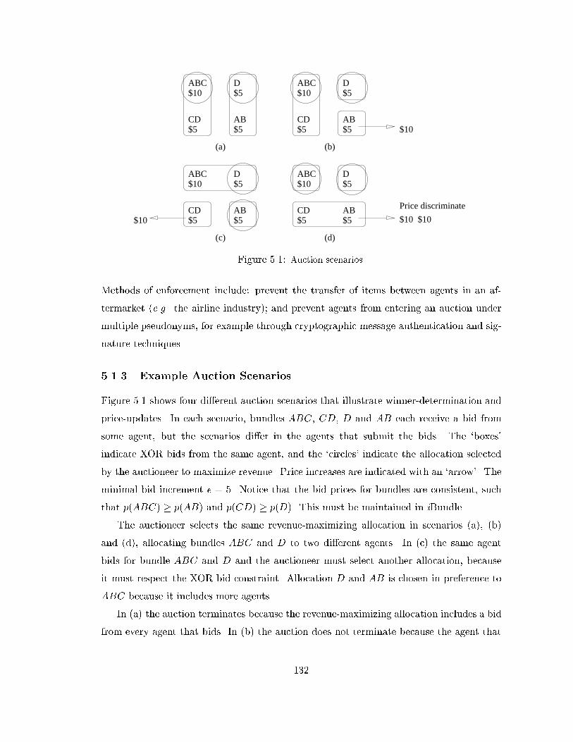
Figure 5.1: Auction scenarios.

Methods of enforcement include: prevent the transfer of items between agents in an af-

termarket (e.g. the airline industry); and prevent agents from entering an auction under

multiple pseudonyms, for example through cryptographic message authentication and sig-

nature techniques.

5.1.3 Example Auction Scenarios

Figure 5.1 shows four di�erent auction scenarios that illustrate winner-determination and

price-updates. In each scenario, bundles ABC, CD, D and AB each receive a bid from

some agent, but the scenarios di�er in the agents that submit the bids. The `boxes'

indicate XOR bids from the same agent, and the `circles' indicate the allocation selected

by the auctioneer to maximize revenue. Price increases are indicated with an `arrow'. The

minimal bid increment � = 5. Notice that the bid prices for bundles are consistent, such

that p(ABC) � p(AB) and p(CD) � p(D). This must be maintained in iBundle.

The auctioneer selects the same revenue-maximizing allocation in scenarios (a), (b)

and (d), allocating bundles ABC and D to two di�erent agents. In (c) the same agent

bids for bundle ABC and D and the auctioneer must select another allocation, because

it must respect the XOR bid constraint. Allocation D and AB is chosen in preference to

ABC because it includes more agents.

In (a) the auction terminates because the revenue-maximizing allocation includes a bid

from every agent that bids. In (b) the auction does not terminate because the agent that

132

bids (AB; $5) is not happy. The ask price for AB is increased to 5 + �, the minimal bid

increment, in the next round. Scenario (c) is similar, except that the provisional allocation

is di�erent, and the price is increased on CD in the next round. In (d) the bids from the

agent that receives no bundle in the provisional allocation are not safe because bundle CD

and AB are compatible. The auctioneer introduces individual prices for this agent in the

next round. The ask price remains unchanged for the agents in the provisional allocation,

but ask prices increase to 5 + � for bundles CD and AB to the third agent.

5.1.4 Worked Examples

Consider Problem 4 in Table 5.1, in which agent 1 wants either A or B, and has value 2

for each, and agent 2 wants only A and B, and has value 3 for AB. The e�cient allocation

is to allocate AB to agent 1. Table 5.2 illustrates the ask prices, allocation, and bids from

agents in each round of iBundle(2). The bid increment is � = 0:5. Notice that agent 1

bids � below the ask price in round 4 because it repeats a bid for a bundle in the current

allocation, and agent 2 takes a discount in round 11 because the ask prices are greater than

its values. The provisional allocation in each round is indicated �. The auction terminates

with the optimal allocation [1; AB] in round 11 because it receives the same bids as in

round 10. The �nal prices are subadditive, in fact as � ! 0 the �nal prices approach

p(A) = p(B) = 2 = p(AB). The ask price on AB remains within � of the maximum (and

not the sum) of the prices on A and B because agent 2 bids for both A and B and the

auctioneer cannot sell multiple bundles to the same agent.

A B AB

Agent 1 0 0 3�

Agent 2 2 2 2

Table 5.1: Problem 4

There are no linear (i.e. prices on items) that support the e�cient allocation in Problem

4 in competitive equilibrium. Actually, there are not even any non-linear and anonymous

prices that support the e�cient allocation in competitive equilibrium. For examples, prices

p(AB) = p(A) = p(B) = 2:1 are not in competitive equilibrium with allocation [1; AB]

because the auctioneer wants to sell A and B separately to maximize revenue. Non-linear

and non-anonymous prices, such as p1(A) = p1(B) = 0; p1(AB) = 2:5 and p2(A) = p2(B) =

p2(AB) = 2:1 are required to support the e�cient allocation in competitive equilibrium.

133

Round Prices Bids Allocation RevenueA B AB Agent 1 Agent 2

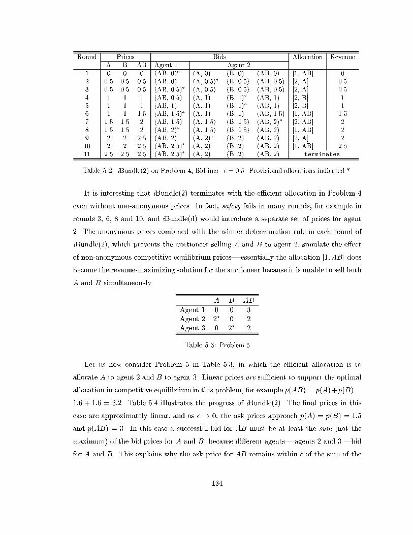
1 0 0 0 (AB, 0)� (A, 0) (B, 0) (AB, 0) [1, AB] 02 0.5 0.5 0.5 (AB, 0) (A, 0.5)� (B, 0.5) (AB, 0.5) [2, A] 0.53 0.5 0.5 0.5 (AB, 0.5)� (A, 0.5) (B, 0.5) (AB, 0.5) [2, A] 0.54 1 1 1 (AB, 0.5) (A, 1) (B, 1)� (AB, 1) [2, B] 15 1 1 1 (AB, 1) (A, 1) (B, 1)� (AB, 1) [2, B] 16 1 1 1.5 (AB, 1.5)� (A, 1) (B, 1) (AB, 1.5) [1, AB] 1.57 1.5 1.5 2 (AB, 1.5) (A, 1.5) (B, 1.5) (AB, 2)� [2, AB] 28 1.5 1.5 2 (AB, 2)� (A, 1.5) (B, 1.5) (AB, 2) [1, AB] 29 2 2 2.5 (AB, 2) (A, 2)� (B, 2) (AB, 2) [2, A] 210 2 2 2.5 (AB, 2.5)� (A, 2) (B, 2) (AB, 2) [1, AB] 2.511 2.5 2.5 2.5 (AB, 2.5)� (A, 2) (B, 2) (AB, 2) terminates.

Table 5.2: iBundle(2) on Problem 4, Bid incr. � = 0:5. Provisional allocations indicated *.

It is interesting that iBundle(2) terminates with the e�cient allocation in Problem 4

even without non-anonymous prices. In fact, safety fails in many rounds, for example in

rounds 3, 6, 8 and 10, and iBundle(d) would introduce a separate set of prices for agent

2. The anonymous prices combined with the winner-determination rule in each round of

iBundle(2), which prevents the auctioneer selling A and B to agent 2, simulate the e�ect

of non-anonymous competitive equilibrium prices| essentially the allocation [1; AB] does

become the revenue-maximizing solution for the auctioneer because it is unable to sell both

A and B simultaneously.

A B AB

Agent 1 0 0 3Agent 2 2� 0 2Agent 3 0 2� 2

Table 5.3: Problem 5

Let us now consider Problem 5 in Table 5.3, in which the e�cient allocation is to

allocate A to agent 2 and B to agent 3. Linear prices are su�cient to support the optimal

allocation in competitive equilibrium in this problem, for example p(AB) = p(A)+p(B) =

1:6 + 1:6 = 3:2. Table 5.4 illustrates the progress of iBundle(2). The �nal prices in this

case are approximately linear, and as � ! 0, the ask prices approach p(A) = p(B) = 1:5

and p(AB) = 3. In this case a successful bid for AB must be at least the sum (not the

maximum) of the bid prices for A and B, because di�erent agents| agents 2 and 3 |bid

for A and B. This explains why the ask price for AB remains within � of the sum of the

134

Round Prices Bids Allocation RevenueA B AB Agent 1 Agent 2 Agent 3

1 0 0 0 (AB, 0) (A, 0)� (AB, 0) (B, 0)� (AB, 0) [2, A], [3, B] 02 0 0 0.5 (AB, 0.5)� (A, 0) (AB, 0.5) (B, 0) (AB, 0.5) [1, AB] 0.53 0.5 0.5 1 (AB, 0.5) (A, 0.5)� (AB, 1) (B, 0.5)� (AB, 1) [2, A], [3, B] 14 0.5 0.5 1 (AB, 1) (A, 0.5)� (AB, 1) (B, 0.5)� (AB, 1) [2, A], [3, B] 15 0.5 0.5 1.5 (AB, 1.5)� (A, 0.5) (B, 0.5) [1, AB] 1.56 1 1 1.5 (AB, 1.5) (A, 1)� (AB, 1.5) (B, 1)� (AB, 1.5) [2, A], [3, B] 27 1 1 2 (AB, 2) (A, 1)� (B, 1)� [2, A], [3, B] 28 1 1 2.5 (AB, 2.5)� (A, 1) (B, 1) [1, AB] 2.59 1.5 1.5 2.5 (AB, 2.5) (A, 1.5)� (AB, 2) (B, 1.5)� (AB, 2) [2, A], [3, B] 310 1.5 1.5 3 (AB, 3) (A, 1.5)� (B, 1.5)� [2, A], [3, B] 311 1.5 1.5 3.5 (AB, 3) (A, 1.5)� (B, 1.5)� terminates.

Table 5.4: iBundle(2) on Problem 5, Bid incr. � = 0:5. Provisional allocations indicated *.

ask prices for A and B throughout the auction.

Notice that bid safety is never violated by the bids from an unsuccessful agent in any

round of iBundle in Problem 5, providing direct evidence that non-anonymous prices are

not required for a competitive equilibrium outcome.

5.2 Theoretical Results

We can make an immediate claim about the e�ciency of iBundle with agents that fol-

low myopic best-response strategies, based on the analysis of the primal-dual algorithm

CombAuction in the previous chapter. See Parkes & Ungar [PU00a] for a direct proof.

Recall that jGj is the number of items, jIj is the number of agents, and � is the minimal

bid increment.

Theorem 5.1 (optimality). iBundle terminates with an allocation that is within

3minfjGj; jIjg� of the optimal solution, for best-response agent bidding strategies.

The auction is optimal as the bid increment approaches zero because the error-term

goes to zero.

As described earlier, the optimality follows from a primal-dual analysis: the provisional

allocation is always a feasible primal solution, the prices a feasible dual solution, and

complementary-slackness conditions hold on termination.

135

In a simpler variation, iBundle(2), the auctioneer never tests for bid-safety and never

introduces price discrimination.

Theorem 5.2 (anonymous optimality). iBundle(2) terminates with an allocation that

is within 3minfjGj; jIjg� of the optimal solution when bids are safe, for best-response agent

bidding strategies.

As noted in the context of CombAuction (Theorem 4.7), special cases on agent pref-

erences for which iBundle(2) remains e�cient, include the following:

(1) Every agent demands di�erent bundles

(2) Agents have additive or superadditive values, i.e. v(S [ S0) � v(S) + v(S0) for non-

con icting bundles S and S0

(3) The bundles that receive bids throughout the auction are from a single partition of

items, e.g. bids are for pairs of matching shoes or individual items.

5.3 Experimental Methods

Experimental results support the theoretical claims about the allocative e�ciency of

iBundle. Results also demonstrate that iBundle continues to perform well with quite large

bid increments, and without price discrimination. The performance of iBundle is tested on

randomly generated problems sets and with myopic best-response agent bidding strategies.

5.3.1 Metrics

Given allocation S = (S1; : : : ; SI) we compute the following metrics:

[E�ciency] Allocative e�ciency, e� (S), is measured as the ratio of the value of the

�nal allocation S to the value V � of the optimal allocation that maximizes total value

across the agents: e� (S) =P

i

vi(Si )=V� where vi(Si) is agent i's value for bundle Si.

[Correctness] Correctness, corr (S), is measured as the average number of times that

an auction �nds the optimal allocation. Correctness can provide a more sensitive measure

of performance than e�ciency.

[Revenue] Revenue, rev(S), is measured as auctioneer's �nal revenue, as a ratio of the

value of the optimal solution: rev(S) =P

i

pi (Si )=V� where pbid;i(Si) is the �nal payment

136

made by agent i for bundle Si.

A simple metric is used to assess information revelation in the auction.

[Information Revelation] Information revelation, inf (i), for agent i is measured as

the sum of the �nal price bid by the agent for all bundles in its valuation function, as a

fraction of the sum of the true value of each bundle:

inf (i) =

P

S2bidi

p�bid;i(S )

P

S2val funi

vi(S )

where p�bid;i(S) is the maximum bid from agent i for bundle S during the auction; bidi

is the set of bundles that receive bids from agent i; and val funi is the set of bundles with

positive value in agent i's valuation function.

The overall information revelation, inf , is computed as the average information reve-

lation over all agents. Asymptotically, if the auction terminates after the �rst round, as

is would in the example in Figure 3.1 in Chapter 3, inf = 0%, while if the auction termi-

nates only after every agent has revealed its complete value for all bundles in its valuation

function, inf = 100%. The information revelation in the GVA is clearly 100%.

In addition to reducing information revelation, we would also like an agent to be able

to follow a myopic best-response strategy in an iterative auction without computing its

exact value for all bundles. Chapter 8 considers the complexity of an agent's best-response

bidding problem. In simple terms, best-response is possible without exact values on all

bundles because an agent must only determine the bundle with a utility (value - price) that

dominates the utility of the other bundles at the current prices. This can be determined

with appropriate upper- and lower- bounds on the value of each bundle. In this chapter I

take information revelation as a proxy for agent valuation. This is reasonable in the limit

because complete information revelation certainly requires that an agent computes exact

values for all bundles.

[Communication Cost] The communication cost is a measure of the number and

size of messages sent between agents and the auctioneer during an auction. A bundle is

de�ned with jGj bits, an item with log2 jGj bits, and a value with log2 Vmax, where Vmax is

the largest possible value (for integer values). In iBundle both price increases and best-

response bids require that only the bundle is speci�ed, which costs jGj bits. This is because

the bid price on a bundle is exactly the ask price in myopic best-response, while the amount

of a price increase is always �. As a fraction of the communication cost in the GVA, we

137

measure the total cost to an agent in iBundle as:

comm i =jGj(nbid + nprice)

jVi jjGj log2 Vmax

where there are nbid bids, nprice increases, and jVij bundles with non-zero value in the

agent's valuation function. In some implementations the price messages may be broadcast,

in which case this communication cost is atomized across all agents.

5.3.2 Problem Sets

iBundle is tested on several problem sets from the literature. The problem set charac-

teristics are summarized in Table 5.5. The CalTech problem set [LPR97] is designed to

represent a hard spatial �tting problem, and has been used to test the AUSM and RAD

bundle auctions [DKLP98]. Problem sets PS1 and PS2 are resource allocation problems

that have been used to test the performance of a sequential auction mechanism (SEQ)

with adaptive agent bidding strategies [BGS99].

Problem sets 4-8 are designed to represent di�erent levels of subadditivity and super-

additivity over items. I refer to these problem sets as k-comp(g). Agents have subadditive

values for combinations of items when k < 1, and superadditive values when k > 1. The

parameter g indicates how many items are covered by bundles with positive value in each

agent's valuation function.

Problem sets 9-16 are generated from bid distributions used to test a new winner deter-

mination algorithm for bundle auctions [San99]. Agent valuation functions are generated

by partitioning the bid distributions across the agents. In problem sets 9{12 agents have

exclusive-or values across bundles, i.e. vi(S [ T ) = max(vi(S); vi(T )), while in problem

sets 13{16 agents have additive-or values, i.e. vi(S[T ) = vi(S)+vi(T ) for disjoint bundles

S \ T = ;.

Larger problem sets than those in Table 5.5 are constructed from Sandholm's Decay,

Random, Uniform, and Weighted-Random distributions, increasing the number of agents

and/or the number of items. In our main experiments the number of items, jGj = 50, and I

scale the problems by increasing the number of agents, jIj, from 5 to 40, with values for 10

bundles per agent. Sandholm's � parameter in the Decay distribution is set to � = 0:85,

and bundles of size 10 are computed in the Uniform distribution.

Table 5.5 states the number of items jGj in each problem set, the number of agents jIj,

the average number of bundles with positive value for each agent, and whether the agents

138

Problem jGj jI j Number (X)or Num Naive Naive Num# Name bundles / agents in e� corr trials

per agent (O)r sol (%) (%) (%)1 CalTech 6 5 5 X 40.0 63.2 2 502 PS1 12 4 3.97 X 89.0 82.1 20 503 PS2 12 5 4.07 X 58.4 79.3 20 504 0-comp(4) 5 5 15 X 85.6 61.2 0 505 0.5-comp(4) 5 5 15 X 80.8 63.2 0 506 1-comp(4) 5 5 15 X 71.2 63.0 0 507 2-comp(4) 5 5 15 X 49.2 65.3 4 508 4-comp(4) 5 5 15 X 43.6 63.5 6 509 random 10 5 10 X 84.8 64.9 8 2510 w-random 10 5 10 X 38.4 82.8 20 2511 uniform 20 5 10 X 60.0 73.0 8 2512 decay 20 5 10 X 96.0 80.2 12 2513 random-or 10 5 10 O 74.4 55.3 0 2514 w-random-or 10 5 10 O 39.2 82.4 20 2515 uniform-or 20 5 10 O 48.8 69.6 4 2516 decay-or 20 5 10 O 92.8 72.5 0 25

Table 5.5: Problem characteristics.

have OR or XOR values over bundles. Table 5.5 also records the average percentage of

agents in the optimal allocation. All other things being equal, we would expect a greater

proportion of agents to receive bundles as the number of items increases, the number of

agents decreases, and the level of superadditivity decreases. For example, the number

of agents in the optimal solution falls as k increases in the k-comp(g) problem sets. I

also compute the performance of a naive central algorithm naive for each problem set, to

provide a baseline for the performance of the auction-based solutions. The naive algorithm

repeatedly selects an agent at random (without replacement) and tries to allocate bundles

to the agent until it is happy, choosing bundles in order of decreasing value.

5.3.3 Comparison Auction Mechanisms

I compared the performance of iBundle with reported results for other auctions. AUSM

and RAD are iterative auctions that allow agents to bid for bundles [LPR97, DKLP98].

SEQ [BGS99] is a sequential auction, in which each item is sold in a sealed-bid auction in

sequence, and agents must learn to anticipate the future prices of items that they need to

complete a bundle when bidding for early items.

I also implemented a simple simultaneous ascending price auction, with and without

bid withdrawal (SAA-w and SAA). In SAA-w agents can withdraw a bid in any round.

139

When an agent withdraws a bid (j; p) for item j 2 G at price p the ask price for the

item in the next round is set to p. If the item remains unsold the agent must pay its

bid price, but otherwise there is no penalty. This approximates the rule used in the FCC

spectrum auction [Plo97]. The best-response bidding strategy in SAA is to bid for items

that maximize utility, assuming they will win every bid. Without budget constraints agents

write-o� incomplete bundles with this strategy, in a phenomena described by Bykowsky et

al. [BCL00] as mutually destructive bidding.

The best-response strategy in SAA-w is similar, except that agents assume that they

can decommit for free. Once an agent has withdrawn a bid, the penalty represents a sunk

cost. There is continued debate about the e�ect of bid withdrawal on auction performance

[BCL00, Por99].

5.3.4 Experimental Platform

iBundle is coded in C++, with a branch-and-bound depth-�rst search used to solve the

auctioneer's winner determination problem in each round. Modules to generate random

problem sets, and simulate agent bidding strategies were also coded in C++. I have also ex-

perimented with the GAMS/CPLEX platform as a method to solve winner-determination

in each round of the auction.

A variation on Sandholm's depth-�rst branch-and-bound search algorithm [San99]

solves winner-determination in each round, and computes the allocation and prices in

the GVA. A new heuristic is introduced to make search more e�cient for XOR bids. The

heuristic computes an overestimate of the possible value of a partial allocation based on

allocating at most one bundle to each remaining agent without a bundle.

5.3.5 Normalized Bid Increment

In some tests it is useful to normalize the minimal bid increment across problem distribu-

tions, to give some consistency in comparisons of allocative e�ciency, etc. The minimal bid

increment � is adjusted to normalize for the number of bundles in an average solution and

the average value of an optimal solution; i.e. an increment of x% represents an actual bid

increment � = xV �=(100W �) where W � is the average number of bundles in the optimal

allocation and V � is the average value of the optimal allocation.

140

Problem Performance SEQ RAD AUSM iBundle(2)# Name measure � (%)

20 5

1 CalTech e� 90.4 94 96.4 99.7corr 80 36 80rev 79 71 70.6 77.7

2 PS1 e� 87 92.4 99.4

3 PS2 e� 80 92.8 99.7

Table 5.6: Performance comparison with SEQ, RAD and AUSM on problems 1, 2 and 3. Bidincrement � (%); E�ciency e� (%); Correctness corr (%); Revenue rev (%).

5.4 Results I: E�ciency and Information Revelation

Table 5.6 compares the performance of iBundle(2) with reported results for AUSM and

RAD [DKLP98, LPR97] on problem set 1 in Table 5.5. The experiments reported in

DeMartini et al. [DKLP98] are with human participants, and it is possible that software

agents could perform better (or worse). This aside, iBundle(2) achieves a higher e�ciency

than RAD and AUSM, and is competitive in revenue. I also compared the performance of

iBundle with SEQ [BGS99] on problem sets 2 and 3. iBundle(2) generates almost perfect

allocations, signi�cantly outperforming SEQ (results on corr and rev are not available for

SEQ). The empirical results reported for SEQ are with agents that follow sophisticated

bidding strategies, learned over many repeated trials of the same problem instance. In

comparison, iBundle agents follow simple best-response bidding strategies.

1 4 8 12 1650

60

70

80

90

100

Problem Set

Effi

cien

cy (

%)

(a)

1 4 8 12 160

20

40

60

80

100

Problem Set

Cor

rect

(%

)

(b)

Figure 5.2: Performance of SAA-w `x', iBundle(2) `+', and a naive central resource allocationalgorithm `o'. Bid increment � = 5%. (a) E�ciency. (b) Correctness.

141

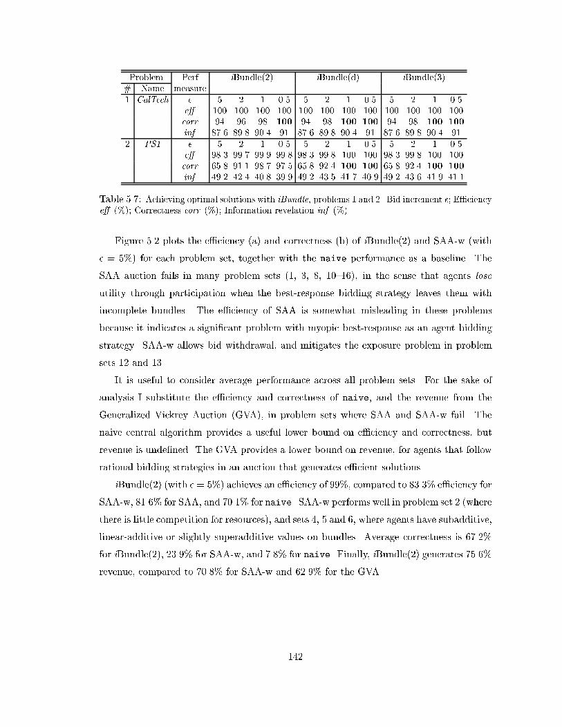
Problem Perf iBundle(2) iBundle(d) iBundle(3)# Name measure1 CalTech � 5 2 1 0.5 5 2 1 0.5 5 2 1 0.5

e� 100 100 100 100 100 100 100 100 100 100 100 100corr 94 96 98 100 94 98 100 100 94 98 100 100

inf 87.6 89.8 90.4 91 87.6 89.8 90.4 91 87.6 89.8 90.4 912 PS1 � 5 2 1 0.5 5 2 1 0.5 5 2 1 0.5

e� 98.3 99.7 99.9 99.8 98.3 99.8 100 100 98.3 99.8 100 100corr 65.8 91.1 98.7 97.5 65.8 92.4 100 100 65.8 92.4 100 100

inf 49.2 42.4 40.8 39.9 49.2 43.5 41.7 40.9 49.2 43.6 41.9 41.1

Table 5.7: Achieving optimal solutions with iBundle, problems 1 and 2. Bid increment �; E�ciencye� (%); Correctness corr (%); Information revelation inf (%).

Figure 5.2 plots the e�ciency (a) and correctness (b) of iBundle(2) and SAA-w (with

� = 5%) for each problem set, together with the naive performance as a baseline. The

SAA auction fails in many problem sets (1, 3, 8, 10{16), in the sense that agents lose

utility through participation when the best-response bidding strategy leaves them with

incomplete bundles. The e�ciency of SAA is somewhat misleading in these problems

because it indicates a signi�cant problem with myopic best-response as an agent bidding

strategy. SAA-w allows bid withdrawal, and mitigates the exposure problem in problem

sets 12 and 13.

It is useful to consider average performance across all problem sets. For the sake of

analysis I substitute the e�ciency and correctness of naive, and the revenue from the

Generalized Vickrey Auction (GVA), in problem sets where SAA and SAA-w fail. The

naive central algorithm provides a useful lower bound on e�ciency and correctness, but

revenue is unde�ned. The GVA provides a lower bound on revenue, for agents that follow

rational bidding strategies in an auction that generates e�cient solutions.

iBundle(2) (with � = 5%) achieves an e�ciency of 99%, compared to 83.3% e�ciency for

SAA-w, 81.6% for SAA, and 70.1% for naive. SAA-w performs well in problem set 2 (where

there is little competition for resources), and sets 4, 5 and 6, where agents have subadditive,

linear-additive or slightly superadditive values on bundles. Average correctness is 67.2%

for iBundle(2), 23.9% for SAA-w, and 7.8% for naive. Finally, iBundle(2) generates 75.6%

revenue, compared to 70.8% for SAA-w and 62.9% for the GVA.

142

10−2

100

102

0

20

40

60

80

100

120

Bid increment

wor

k auct

ione

er

(iii)

10−2

100

102

0

20

40

60

80

Bid increment

Info

rmat

ion

Rev

elat

ion

(%)

(ii)

10−2

100

102

0

20

40

60

80

100

Bid increment

(%)

(i)

Correct

Efficiency

10−2

100

102

0

1000

2000

3000

4000

5000

6000

Bid incrementco

mm

agen

t (%

)

(iv)

Figure 5.3: Performance of iBundle as the bid increment � decreases. `+' iBundle(2); `�' iBun-dle(d); `�' iBundle(3). Problem 0.5-comp(3).

5.4.1 E�ect of Price Discrimination

Figure 5.3 (i) compares the e�ciency and correctness across each auction variation for prob-

lem set 0.5-comp(3), which is a problem with 5 agents, 5 items, and 7 bundles/agent. Al-

though price discrimination is required for 100% correctness in this problem, the e�ciency

improvement is negligible. The increase in e�ciency with iBundle(d) and iBundle(3),

compared to iBundle(2) is marginal. With � = 5%, iBundle(3) achieves 99.1% e�ciency,

compared to 99% e�ciency for iBundle(2). Table 5.7 presents similar results for Problems

1 and 2.

Price discrimination only makes a di�erence for very small bid increments, when the

communication cost begins to increase rapidly. For bid increment � > 0:5% the perfor-

mance is almost identical. The relationship between average number of rounds to termi-

nation and bid increment is approximately linear, with � = 5%; 0:5%; 0:05% corresponding

to 6, 49, and 480 rounds respectively. An auctioneer may choose not to operate below

0:5% because of high communication costs, computation costs, and indirect costs due to

elapsed time.

143

Figure 5.3 (ii) plots the information revelation; (iii) the auctioneer's computation cost;

and (iv) the agent's communication cost. The computation cost in this experiment is as-

sumed to scale exponentially with the worst-case size of the winner-determination problem

solved in iBundle, and with the size of the winner-determination problem with all agents

in the GVA. Size is measured as the product of the number of bids received (or bundles

with values in the GVA) and the number of items. Finally, the cost is normalized on a

log-scale, with the cost of the GVA equaling 100%. We might expect the worst-case run-

time in iBundle to be dominated by the time on the largest problem in any round because

winner-determination is NP-hard. Similarly, the cost of solving WD for all agents should

dominate in the GVA.

The results show that iBundle can tradeo� performance for communication, compu-

tation, and information revelation costs. iBundle(2) achieves allocations that average

91.7% e�ciency across all problem sets and terminates after 5.7 rounds with bid incre-

ment � = 20%, down from 99% e�ciency after 18 rounds with bid increment � = 5%.

Price discrimination only helps for bid increments less than around � = 0:5, at which point

the communication cost begins to increase rapidly. It is likely that an auctioneer would

choose not to operate in this region anyway. The performance of all auction variations

is approximately identical in the region with reasonable communication cost. As the bid

increment decreases we can achieve a continuous tradeo� between performance (e�ciency

and correctness), information revelation, and communication cost. Notice also that the

dynamic and third-order iBundle auctions require more information revelation and auc-

tioneer computation than the second-order iBundle auction in this problem domain, but

have less communication cost.

5.4.2 Information Revelation

iBundle(2) requires an average of 57.5% information revelation at � = 20% (when the allo-

cations are 91.7% e�cient), and an average of 71% information revelation at � = 5% (when

the allocations are 99% e�cient). The (sealed-bid) GVA requires 100% information reve-

lation from agents to achieve 100% e�ciency. I would expect information revelation to be

smaller in real-world problems. The agents in the problem sets have sparse valuation func-

tions, which limits the size of the worst-case information revelation, i.e. the denominator in

the information-revelation metric. In addition, information revelation would be smaller in

144

Problem jGj jIj Number (X)or Num Naive Naive Num# Name bundles / agents in e� corr trials

per agent (O)r sol (%) (%) (%)

17 decay(2) 20 2 25 X 100 93.0 64 2518 decay(10) 20 10 5 X 77.2 75.5 4 2519 decay(25) 20 25 2 X 37.4 61.2 0 2520 decay(50) 20 50 1 X 20.6 62.8 0 25

Table 5.8: Problems for the easy-hard scalable performance test.

\easier" problems, for example with signi�cant over-demand or signi�cant under-demand.

In the former only a few agents need to drive the price adjustment, while in the latter we

would expect iBundle to terminate quickly because it is likely that an early provisional

allocation would include bids from all agents.

One of the main claims for iterative auctions vs. sealed bid auctions is that they provide

major computational advantages in easy problem instances, terminating quickly with little

information revelation and computation. To test this claim I studied the Decay problem

set as the number of agents increased from 2 to 50. Table 5.8 summarizes the statistics

for the problems. The problem is relatively easy with a few agents, but as the number of

agents increases the level of competition increases and it is more di�cult to compute the

optimal solution. For example, all agents are in the optimal allocation with a few agents,

and the e�ciency and correctness of the naive algorithm is high.

Figure 5.4 illustrates the performance of iBundle as the \di�culty" of the combinatorial

allocation problem is increased. In each trial I select a bid increment to make iBundle

compute a solution with the same quality, i.e. with a similar e�ciency and correctness,

see Figure 5.4 (i).

As the instances get more di�cult the auctioneer's computational cost steadily in-

creases, see Figure 5.4 (iii). As described above, this is measured as the size of the largest

winner-determination problem the auctioneer must solve, as a fraction of the size of the

problem in the GVA (with full valuation functions from each agent). In easy problems the

largest winner-determination problems in iBundle are about half the size of the problems

in the GVA, which could be signi�cant for an NP-hard problem.

Communication cost in iBundle(2) and iBundle(d) is a linear function of the number

of agents, see Figure 5.4 (iv), essentially because a cost is accounted to send price updates

to all agents. This is not a very accurate measure, as simple methods that allow agents

145

0 10 20 30 40 500

200

400

600

800

1000

1200

Problem Complexity (Number of Agents)co

mm

agen

t (%

)

(iv)

0 10 20 30 40 5030

40

50

60

70

80

90

100

Problem Complexity (Number of Agents)

(%)

(i)

Efficiency

Correct

0 10 20 30 40 5010

20

30

40

50

60

Problem Complexity (Number of Agents)

Info

rmat

ion

Rev

elat

ion

(%)

(ii)

0 10 20 30 40 500

20

40

60

80

100

120

Problem Complexity (Number of Agents)

wor

k auct

ione

er

(iii)

Figure 5.4: Performance of iBundle as the problem di�culty is increased. `+' iBundle(2); `�'iBundle(d); `�' iBundle(3). Decay problem set, for 2, 10, 25, and 50 agents.

to drop out of the auction will give similar communication costs across iBundle(2), (d)

and (3). Essentially, the communication scaling properties are strongly sublinear in the

number of agents, because many agents quickly drop out as prices get too high.

Figure 5.4 (ii) plots the e�ect on information revelation in iBundle as the problem

complexity varies. The most interesting e�ect can be observed between 0 and 10 agents.

For less than 10 agents the problem is solved with very little information from agents. The

peak information revelation occurs for problems of intermediate size, when every agent in

the system must report quite accurate and complete information. As the number of agents

increase the average information revelation falls because information from some agents

becomes irrelevant.

146

5.5 Results II: Winner Determination and Communication

Cost

The auctioneer must solve one WD problem in each round, and a naive worst-case analysis

gives O(BVmax=�) rounds to converge, for a total of B bundles with positive value over

all agents, maximum value Vmax for any bundle, minimal bid increment �, and myopic

best-response. In the worst-case the price of a single bundle must increase by at least � in

each round the auction remains open, and prices are bounded by the maximum value over

all agents. The number of rounds to termination is inversely proportional to the minimal

bid increment.

The auctioneer announces only price increases in each round, and does not maintain

explicit prices for all possible bundles. Instead, bid prices are veri�ed dynamically in each

round, to check that bids are at least as large as the ask price of all contained bundles.

The total work in checking each bid is linear in the number P of bundles that have explicit

ask prices, with a naive linked-list data structure. Similarly, price monotonicity can be

maintained in linear time in P for each new price increase. In addition, P � B, with

agents that have values for B bundles, because only bundles that receive bids can receive

explicit ask prices.

The winner-determination (WD) problem that the auctioneer solves in each round of

iBundle is NP-hard, itself a small instance of the CAP problem. However, each problem

is smaller than the problems in the GVA, because the winner-determination problem is

revenue-maximization given agents' best-response bids, while in the GVA the problem is to

compute the e�cient allocation directly from valuation functions. However, the problem

instances might also be hard instances because all agents bid at similar prices for bundles

(Andersson et al. [ATY00]), which can restrict the ability of search-based methods to

prune the search space.

The following sections describe a number of interesting methods to speed-up the winner-

determination problem in iBundle. First, the provisional allocation from the previous

round provides a good initial solution to the WD problem, because agents must re-bid

bundles received in the previous round. This allows pruning of the search for a revenue-

maximizing allocation. An additional saving in computation time is achieved by limiting

search to an allocation at least � better than the value of the allocation in the previous

147

round. Approximations can be introduced to speed-up winner-determination, both through

increasing the minimal bid increment and decreasing the number of winner-determination

problems to solve (one in each round), and with approximate winner-determination algo-

rithms. Another approach is to cache provisional allocations from previous rounds, and

use cached solutions to compute good initial solutions in the current round of the auction.

One interesting heuristic suggested by an analysis of the hit statistics of the cache is the

\ ip- op" heuristic, which adopts a cache hit as the new provisional allocation without

additional search.

5.5.1 Minimal Bid Increment Approximations

5 10 15 20 25 30 35 4010

0

101

102

103

104

105

106

Number of Agents

Auc

tione

er C

PU

Tim

e (s

)

80%

85%

Truthful

95%99%

GVA

Figure 5.5: Total computation time in iBundle(2), the GVA, and a sealed-bid auction with truthfulagents, in problem set Decay. The performance of iBundle is plotted with di�erent bid increments�, selected to give allocative e�ciency of 80%, 85%, 95% and 99%.

One method to introduce approximations is via the minimal bid increment. Figure 5.5

plots the total auctioneer winner-determination and price-update time2 in iBundle in the

Decay problem set. Performance is measured for di�erent bid increments, with the bid

increment selected to give allocative e�ciency of 80%, 85%, 95% and 99% (�1%). Figure

5.5 also plots performance for the GVA, and for a sealed-bid auction in which agents are

assumed to bid truthfully. The GVA proved intractable for 30 and 40 agents. In those

problems the run time is estimated as the time to compute the optimal solution in a single

2Time is measured as user time in seconds on a 450 MHz Pentium Pro with 1024 MRAM, with iBundlecoded in C++.

148

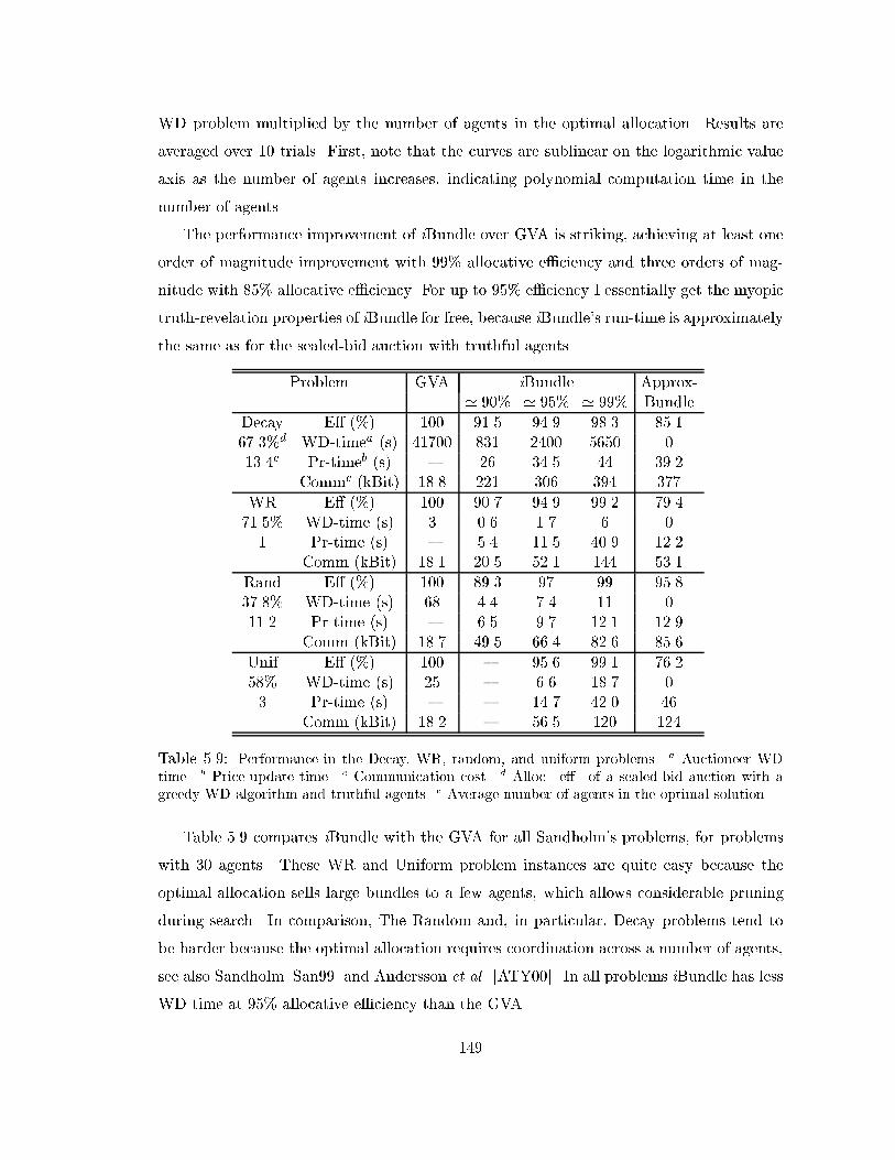
WD problem multiplied by the number of agents in the optimal allocation. Results are

averaged over 10 trials. First, note that the curves are sublinear on the logarithmic value

axis as the number of agents increases, indicating polynomial computation time in the

number of agents.

The performance improvement of iBundle over GVA is striking, achieving at least one

order of magnitude improvement with 99% allocative e�ciency and three orders of mag-

nitude with 85% allocative e�ciency. For up to 95% e�ciency I essentially get the myopic

truth-revelation properties of iBundle for free, because iBundle's run-time is approximately

the same as for the sealed-bid auction with truthful agents.

Problem GVA iBundle Approx-' 90% ' 95% ' 99% Bundle

Decay E� (%) 100 91.5 94.9 98.3 85.167.3%d WD-timea (s) 41700 831 2400 5650 013.4e Pr-timeb (s) { 26 34.5 44 39.2

Commc (kBit) 18.8 221 306 394 377

WR E� (%) 100 90.7 94.9 99.2 79.471.5% WD-time (s) 3 0.6 1.7 6 01 Pr-time (s) { 5.4 11.5 40.9 12.2

Comm (kBit) 18.1 20.5 52.1 144 53.1

Rand E� (%) 100 89.3 97 99 95.837.8% WD-time (s) 68 4.4 7.4 11 011.2 Pr-time (s) { 6.5 9.7 12.1 12.9

Comm (kBit) 18.7 49.5 66.4 82.6 85.6

Unif E� (%) 100 { 95.6 99.1 76.258% WD-time (s) 25 { 6.6 18.7 03 Pr-time (s) { { 14.7 42.0 46

Comm (kBit) 18.2 { 56.5 120 124

Table 5.9: Performance in the Decay, WR, random, and uniform problems. a Auctioneer WDtime. b Price-update time. c Communication cost. d Alloc. e�. of a sealed-bid auction with agreedy WD algorithm and truthful agents. e Average number of agents in the optimal solution.

Table 5.9 compares iBundle with the GVA for all Sandholm's problems, for problems

with 30 agents. These WR and Uniform problem instances are quite easy because the

optimal allocation sells large bundles to a few agents, which allows considerable pruning

during search. In comparison, The Random and, in particular, Decay problems tend to

be harder because the optimal allocation requires coordination across a number of agents,

see also Sandholm [San99] and Andersson et al. [ATY00]. In all problems iBundle has less

WD time at 95% allocative e�ciency than the GVA.

149

Note that the price-update step is relatively expensive in the otherwise easy weighted-

random (WR) problem, because bid prices for large bundles must be checked for price

consistency against the price of all included bundles.

5.5.2 Approximate Winner-Determination

Another method to introduce approximation is via a greedy winner-determination algo-

rithm in each round of the auction.

The auctioneer can maintain the same incentives for myopic agents to follow the same

bidding strategy for any approximation algorithm with the bid-monotonicity property:

Definition 5.2 [bid-monotonicity] An algorithm for winner-determination satis�es bid-

monotonicity if whenever an agent i is allocated a bundle with bids Bi, it is also allocated

a bundle with bids Bi [B that include a bid for an additional bundle B.

It is straightforward to prove that optimal winner-determination algorithms are bid-

monotonic. One simple algorithm with the bid-monotonicity property is due to Lehmann

et al. [LOS99], which allocates bundles in order of decreasing value-per-item.

Table 5.9 presents the e�ciency in iBundle with this approximation algorithm for

winner-determination. Notice that iBundle computes a fast solution to all problems with

the approximate winner-determination algorithm, even in the hard Decay problem set.

The average allocative-e�ciency of iBundle with the approximate winner-determination

algorithm in Decay is a quite respectable 85.1% (notice that a greedy centralized solution

with truthful agents achieves only 67.3%), and with more than a 1000-fold reduction in

winner-determination time. I believe that other, slightly less greedy, approximate algo-

rithms will give even further performance improvements.

5.5.3 Methods to Speed-up Sequential Winner-Determination

The sequential nature of winner-determination in iBundle suggests that cache-based meth-

ods can speed-up winner-determination. I experimented with a cache of all provisional

allocations computed in previous rounds. The auctioneer �rst checks the cache when new

bids are submitted. This provides an initial solution for winner-determination and is used

to prune search. A simple linear program is used to select the best allocation from the

cache.

150

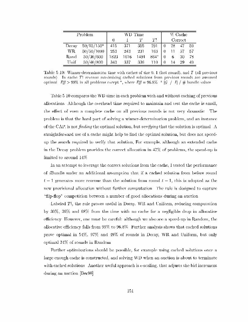
Problem WD Time % Cache0 1 T T ! Correct

Decay 50/15/150a 415 371 355 291 0 28 47 59WR 50/50/1000 253 243 231 163 0 11 57 57Rand 50/30/600 1823 1616 1491 864� 0 6 30 78Unif 50/40/800 343 337 336 110 0 14 29 49

Table 5.10: Winner-determination time with caches of size 0, 1 (last round), and T (all previousrounds). In cache T ! revenue maximizing cached solutions from previous rounds are assumedoptimal. E� > 99% in all problems except �, where E� = 96:8%. a jGj / jI j / # bundle values.

Table 5.10 compares the WD time in each problem with and without caching of previous

allocations. Although the overhead time required to maintain and test the cache is small,

the e�ect of even a complete cache on all previous rounds is not very dramatic. The

problem is that the hard part of solving a winner-determination problem, and an instance

of the CAP, is not �nding the optimal solution, but verifying that the solution is optimal. A

straightforward use of a cache might help to �nd the optimal solution, but does not speed-

up the search required to verify that solution, For example, although an extended cache

in the Decay problem provides the correct allocation in 47% of problems, the speed-up is

limited to around 14%.

In an attempt to leverage the correct solutions from the cache, I tested the performance

of iBundle under an additional assumption that if a cached solution from before round

t � 1 generates more revenue than the solution from round t � 1, this is adopted as the

new provisional allocation without further computation. The rule is designed to capture

\ ip- op" competition between a number of good allocations during an auction.

Labeled T !, the rule proves useful in Decay, WR and Uniform, reducing computation

by 30%, 36% and 68% from the time with no cache for a negligible drop in allocative

e�ciency. However, one must be careful: although we also see a speed-up in Random, the

allocative e�ciency falls from 99% to 96:8%. Further analysis shows that cached solutions

prove optimal in 54%, 97% and 49% of rounds in Decay, WR and Uniform, but only

optimal 34% of rounds in Random.

Further optimizations should be possible, for example using cached solutions once a

large enough cache is constructed, and solving WD when an auction is about to terminate

with cached solutions. Another useful approach is �-scaling, that adjusts the bid increment

during an auction [Ber90].

151

5.5.4 Communication cost

Communication cost is computed using the metric speci�ed in Section 5.3.1, with 10 bits

to specify a value in the GVA. Cost is measured as jGjnbids for each agent plus jGjnprices,

given nbids bids and nprices prices. I assumed that prices are broadcast to agents, and

assess the cost of price information independently of the number of agents in an auction.

Only the cost of bids is counted in iBundle(3), with non-anonymous prices, because the

price changes are implicit in the new provisional allocation. An agent's new prices are �

above its bid price whenever its bids are unsuccessful.

There is a communication cost penalty in using iBundle compared with the GVA in

these problems (Table 5.9) because of repeated bids across a number of rounds. This would

change in problems with agents that have values for many bundles because all values must

be reported in the GVA, or in easier problems because iBundle will terminate quickly with

less bids.

5.6 Special Cases for Expressive Bid Languages

It is possible to derive fast special cases of iBundle for restrictions on agent bidding lan-

guages, which solve the combinatorial allocation problem for assumptions about agent

preferences. The advantage of identifying special cases is that the winner-determination

problem is tractable for particular structures on bundles and price functions over bundles

(see Section 4.5).

5.6.1 Unit-Demand Preferences (Assignment Problem)

In problems where agents have single-unit demands (the standard assignment problem) we

can restrict iBundle in two ways (leading to two di�erent auction mechanisms):

� Restrict agents to placing OR bids on items. In this case iBundle(2) reduces to a si-

multaneous ascending-price auction, that was shown to be optimal for the assignment

problem by Crawford & Knoer [CK81].

� Restrict agents to placing XOR bids on items. In this case the winner-determination

problem in iBundle(2) can be formulated as a max- ow problem, and solved e�-

ciently.The auction only generates prices on items, and is a variant on the auction

152

proposed by Demange et al. [DGS86].

5.6.2 Linear-Additive Preferences

In problems where agents have linear-additive demands on items we can restrict agents

to OR bids on items. The auction reduces to a simultaneous ascending-price auction,

equivalent to Crawford & Knoer's [CK81] auction for the problem.

5.6.3 Gross Substitutes Preferences

Gross substitutes (GS) preferences implies that an agent that demands bundle S in round

t will continue to demand items in S that do not increase in price as the price of other

items increases [KC82]. Linear-additive and unit-demand preferences are special-cases of

gross substitutes. Kelso & Crawford prove GS are a su�cient condition for the existence of

linear competitive equilibrium prices. Again, we can restrict agents to OR bids on items:

� Agents bid for all the items in the single bundle that maximizes their utility in each

round. Gross substitutes implies that an agent will continue to demand any subset

of the items as the price of other items increases, and be happy to continue to bid

for items it receives in a partial allocation. In this case iBundle(2) reduces to a

simultaneous ascending-price auction, that was shown to be optimal for GS by Kelso

& Crawford [KC82].

5.6.4 Multiple Homogeneous Goods

The multiple homogenous good allocation problem is to allocate jGj identical items across

agents, to maximize the total value over all agents. Each agent has a valuation function

vi(m) � 0 de�ned for (integer) quantities m � 0 of the item.

A suitable bidding language allows an agent to submit exclusive-or bids of type (m; p),

which states that the agent will pay at most p for a bundle of at least m items. Essentially,

each bid represents a set of exclusive-or bids over all bundles of items in G of size m. The

winner-determination problem is a multi-unit allocation problem, where each agent must

receive exactly the number of items in its bid. Finally, prices are increased on unsuccessful

bids, with prices maintained for each possible size of bundle (with non-anonymous prices

of the same kind also introduced dynamically). Again, we do not want to maintain an

explicit price for each distinct set of bundles of the same size.

153

An unsuccessful bid at price p on bundles of sizem > (jGj=2) indicates that the minimal

bid price on all bundles of size m must be at least p+� in future rounds. It is not necessary

to announce, or maintain, explicit prices on all possible bundles of size m, but rather just

announce a price on bundles of sizem. Notice thatm > (jGj=2) implies the safety condition

holds over the underlying exclusive-or set of bundles.

An unsuccessful bid at price p on bundles of size m � (jGj=2) must be handled a little

more carefully because it remains possible for the same bid from two di�erent agents at

that price to be successful. We must introduce separate prices for this agent, and increase

its ask price on bundles of size m by �. Notice thatm � (jGj=2) implies the safety condition

does not hold over the underlying exclusive-or set of bundles.

E�ectively, we might expect bids in this auction design to start-o� anonymous while

agents bid for large bundles of items at low prices, and then become more non-anonymous

as agents begin to bid for smaller bundles as the prices increase on large bundles. Even-

tually, it is quite possible that the auction will terminate with di�erent prices to di�erent

agents for bundles of the same size. The exact details of this auction, and an e�cient

implementation, are left for future work.

5.7 Earlier Iterative Combinatorial Auctions

Rassenti et al. [RSB82] propose a sealed-bid bundle auction for the problem of allocating

airport slots, where airlines value take-o� and landing slots in pairs. Agents submit sealed

XOR bids for bundles of take-o� and landing slots. The auction computes linear prices

that approximately clear the market, given agent bids. Finally, agents can place bids and

asks for individual slots in a secondary market, to cleanup their �nal allocation. Although

the auction design is fairly ad-hoc, empirical results with human bidders suggest that the

market can achieve high e�ciency with experienced bidders.

The recent FCC spectrum auction generated a lot of debate among economists about

combinatorial auction mechanisms. Spectrum licenses have non-additive value in bundles

because of network synergies from spatially-coherent geographical regions. The �nal FCC

auction design was a variant on a simultaneous ascending-price auction that allowed agents

limited decommitment rights, and placed participation constraints on agents to enable

information exchange via prices during the auction [MM96]. The goal was to allow agents

154

to �nd a good \�t" between their demand sets and the demand sets of other bidders, and

win coherent bundles of spectrum licenses.

Bykowsky et al. [BCL00] demonstrate the exposure and existence problem with linear

prices for the combinatorial allocation problem, and study the AUSM auction [BLP89]

as an example of a bundle auction to address the problem. AUSM allows agents to bid

for arbitrary bundles of items, and maintains a revenue-maximizing allocation. There

are no pricing rules, and agents must coordinate their own bids. Theoretical analysis

is di�cult because of the exible auction rules, but see Milgrom [Mil00b]. AUSM has

reasonable performance empirically, see Ledyard et al. [LPR97]. Bykowsky et al. identify

the \threshold problem" for bundle auctions, where smaller bidders must coordinate bids

to outbid a larger bidder. Although iBundle solves this problem for agents that follow

best-response bidding strategies, the e�ect of alternative agent bidding strategies on the

threshold (or coordination) problem is unknown.

Recently, DeMartini et al. [DKLP98] proposed RAD, an auction that allows agents to

place XOR bids on bundles but generates prices on items. Although promising empirical

results have been presented, there are no theoretical results on its allocative e�ciency.

RAD also borrows from the FCC auction design, agents must re-submit winning bids,

and there are activity rules to encourage information revelation early in the auction and

encourage coordinate bidding.

Wurman's AkBA combinatorial auction was discussed in Section 4.7. It allows exclusive-

or bids on bundles of items in each round, and maintains anonymous prices on bundles. A

linear-program based price-update rule is used to adjust prices across rounds.

Appendix: Dynamic Price Discrimination

In the Appendix to this chapter I illustrate the dynamic rule for introducing non-anonymous

prices in iBundle on a simple set of parameterized problems, which demonstrate the im-

portance of price-discrimination to achieve allocative-e�ciency in some problems.

Consider Problem 6 in Table 5.11, in which the value of agent 2 for bundleBC, v2(BC),

can take integer values between 5 and 10. The values for bundles not explicitly listed are

consistent with free disposal of items, i.e. v(S0) � v(S) for all S0 � S. The optimal

allocation is ([1; AC]; [2; B]) for every value v2(BC) in this range. The problem is a hard

155

coordination problem because: agent 1 values B more highly than agent 2, but the optimal

solution allocates B to agent 2; and both agents value BC more than any other bundle

but receive another bundle in the optimal allocation.

A B AC BC

Agent 1 2 9 8� 10Agent 2 2 5� 3 v2(BC)

Table 5.11: Problem 6. Agent values, with 5 � v2(BC) � 10. E�cient allocation indicated �.

In this problem �rst- and second-order CE prices exist for v2(BC) � 7, but only third-

order CE prices exist for v2(BC) > 7. For example, when v2(BC) = 6 and v2(BC) = 7,

then p(A) = 2; p(B) = 5, and p(C) = 2 are CE prices. However, when v2(BC) = 8,

no �rst- or second-order CE prices exist, and v(LP1) = v(LP2) = 13:5 > v(IP ) = 13.

It is not possible to price BC high enough (so that agent 2 demands B but not BC)

without making the auctioneer's revenue from selling A and BC together greater than its

revenue from selling B and AC together. Third-order CE prices for v2(BC) = 8 include

p1 = (2; 9; 8; 10) and p2 = (0; 3; 1; 6) for bundles A;B;AC and BC, with other prices set

high enough to satisfy pi(S0) � pi(S) for all S

0 � S.

Although iBundle(2) solves the problem when v2(BC) = 6, the auction fails when

v2(BC) � 7, terminating with allocation ([1; BC]; [2; A]). Auction iBundle(d), with price

discrimination, solves the problem. The auction switches to price discrimination, and

separates the e�ect of agent 1's bids from ask prices to agent 2. Agent 2 continues to bid

for B and the auction terminates with the optimal allocation ([1; AC]; [2; B]).

Table 5.12 (a) shows iBundle(2) for Problem 6 in Table 5.11, for v2(BC) = 7. The

auction fails even though second-order CE prices exist. Price-updates are not safe, for

example in rounds t + 1 and t + 3, so we might expect the auction to terminate with a

suboptimal allocation. Agents 1 and 2 compete on bids for BC, and agent 1 also drives up

the price on B and AC and prevents agent 2 from bidding for B because v1(BC)�v1(B) <

v2(BC)� v2(B). The auction terminates with the suboptimal allocation ([1; BC]; [2; A]),

because agent 2 bids for item A but not B.

Table 5.12 (b) shows the auction for Problem 6 with v2(BC) = 6. In this case the

auction solves the problem. Agent 2 can bid B in all rounds of the auction because

v2(BC) � v2(B) � v1(BC) � v1(B), and the revenue to the auctioneer from allocation

([1; AC]; [2; B]) eventually exceeds the revenue from ([1; BC]) or ([2; BC]). The auction

156

Round Prices Bids RevenueA B AC BC Agent 1 Agent 2

t� 1 (BC, 4.4)� 4.4t 0 3.4 2.4 4.4 (B, 3.4) (AC, 2.4) (BC, 4.4)� (BC, 4.4) 4.4

t+ 1 0 3.4 2.4 4.6 (B, 3.4) (AC, 2.4) (BC, 4.4) (BC, 4.6)� 4.6t+ 2 0 3.6 2.6 4.6 (B, 3.6) (AC, 2.6) (BC, 4.6)� (BC, 4.6) 4.6t+ 3 0 3.6 2.6 4.8 (B, 3.6) (AC, 2.6) (BC, 4.6) (A, 0) (BC, 4.8)� 4.8t+ 4 0 3.8 2.8 4.8 (B, 3.8) (AC, 2.8) (BC, 4.8)� (A, 0)� (BC, 4.8) 4.8

(a) v2(BC) = 7. iBundle(2) fails.

Round Prices Bids RevenueA B AC BC Agent 1 Agent 2

t� 1 (BC, 2.4)� 2.4t 0 1.4 0.4 2.4 (B, 1.4) (AC, 0.4) (BC, 2.4)� (B, 1.4) (BC, 2.4) 2.4

t+ 1 0 1.6 0.4 2.6 (B, 1.6) (AC, 0.4) (BC, 2.4) (B, 1.6) (BC, 2.6)� 2.6t+ 2 0 1.8 0.6 2.6 (B, 1.8) (AC, 0.6) (BC, 2.6)� (B, 1.8) (BC, 2.6) 2.6t+ 3 0 2.0 0.6 2.8 (AC, 0.6) (BC, 2.6) (B, 2.0) (BC, 2.8)� 2.8t+ 4 0 2.0 0.8 2.8 (B, 2) (AC, 0.8)� (BC, 2.8) (B, 2)� (BC, 2.8) 2.8

(b) v2(BC) = 6. iBundle(2) works.

Table 5.12: iBundle(2) on Problem 6. Bid incr. � = 0:2. Provisional allocations indicated *.

terminates with optimal allocation ([1; AC]; [2; B]).

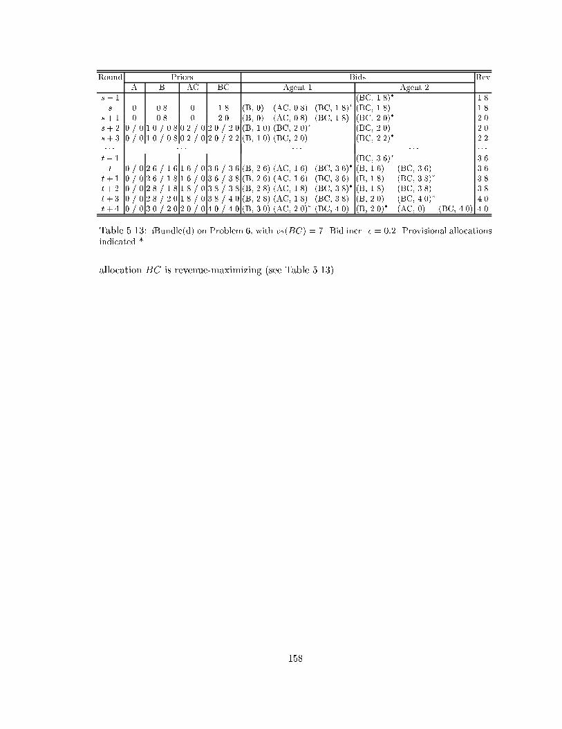
Table 5.13 shows the performance of iBundle(d) in Problem 6 (Table 5.11) for v2(BC) =

7. I use '/' to indicate the prices for each agent. The e�ect of price discrimination is to

separate the price increases caused by bids from agent 1 from the price increases to agent

2. In particular, agent 1's bids for B do not increase the price of B to agent 2, and agent 2

can continue to bid for B (unlike in iBundle(2) on this problem). The auction terminates

with the optimal allocation ([1; AC]; [2; B]).

It is interesting to examine the �nal prices in the auction, to check how well the auction

minimizes CE prices. A methodAdjust is introduced in the next chapter which will adjust

prices after iBundle(3) terminates to minimal CE prices in all CAP problems. We will also

begin to explore the connections between minimal CE prices and Vickrey payments.

In Problem 6, when v2(BC) = 7, the auction terminates with ask prices are p1 =

(0; 3; 2; 4) and p2 = (0; 2; 0; 4) for bundles A;B;AC and AB. Agent values are v1(2; 9; 8; 10)

and v2 = (2; 5; 3; 7). These are minimal CE prices because any lower prices that maintain

best-response changes the revenue-maximizing allocation from ([1; AC]; [2; B]) to an allo-

cation of BC to one of the agents. In fact, the auction increases prices to agents while the

157

Round Prices Bids RevA B AC BC Agent 1 Agent 2

s� 1 (BC, 1.8)� 1.8s 0 0.8 0 1.8 (B, 0) (AC, 0.8) (BC, 1.8)� (BC, 1.8) 1.8

s+ 1 0 0.8 0 2.0 (B, 0) (AC, 0.8) (BC, 1.8) (BC, 2.0)� 2.0s+ 2 0 / 0 1.0 / 0.8 0.2 / 0 2.0 / 2.0 (B, 1.0) (BC, 2.0)� (BC, 2.0) 2.0s+ 3 0 / 0 1.0 / 0.8 0.2 / 0 2.0 / 2.2 (B, 1.0) (BC, 2.0) (BC, 2.2)� 2.2� � � � � � � � � � � � � � �

t� 1 (BC, 3.6)� 3.6t 0 / 0 2.6 / 1.6 1.6 / 0 3.6 / 3.6 (B, 2.6) (AC, 1.6) (BC, 3.6)� (B, 1.6) (BC, 3.6) 3.6

t+ 1 0 / 0 2.6 / 1.8 1.6 / 0 3.6 / 3.8 (B, 2.6) (AC, 1.6) (BC, 3.6) (B, 1.8) (BC, 3.8)� 3.8t+ 2 0 / 0 2.8 / 1.8 1.8 / 0 3.8 / 3.8 (B, 2.8) (AC, 1.8) (BC, 3.8)� (B, 1.8) (BC, 3.8) 3.8t+ 3 0 / 0 2.8 / 2.0 1.8 / 0 3.8 / 4.0 (B, 2.8) (AC, 1.8) (BC, 3.8) (B, 2.0) (BC, 4.0)� 4.0t+ 4 0 / 0 3.0 / 2.0 2.0 / 0 4.0 / 4.0 (B, 3.0) (AC, 2.0)� (BC, 4.0) (B, 2.0)� (AC, 0) (BC, 4.0) 4.0

Table 5.13: iBundle(d) on Problem 6, with v2(BC) = 7. Bid incr. � = 0:2. Provisional allocationsindicated *.

allocation BC is revenue-maximizing (see Table 5.13).

158