chapter 5 array processors. introduction major characteristics of simd architectures –a single...
TRANSCRIPT

Chapter 5 Array Processors
Introduction
Major characteristics of SIMD architectures– A single processor(CP)– Synchronous array processors(PEs)– Data-parallel architectures– Hardware intensive architectures– Interconnection network

Associative Processor
An SIMD whose main component is an associative memory.(Figure 2.19)
AM(Associative Memory): Figure 2.18– Used in fast search operations – Data register– Mask register– Word selector– Result register
Introduction(continued)
Associative processor architectures also belong to the SIMD classification. – STRAN– Goodyear Aerospace’s MPP(massively
parallel processor)The systolic architectures are a
special type of synchronous array processor architecture.
5.1 SIMD Organization
Figure 5.1 shows a SIMD processing model. (Compare to Figure 4.1)
Example 5.1 – SIMDs offer an N-fold throughput
enhancement over SISD provided the application exhibits a data-parallelism of degree N.

5.1 SIMD Organization (continued)
Memory– Data are distributed among the
memory blocks– A data alignment network allows any
data memory to be accessed by any PE.
5.1 SIMD Organization (continued)
Control processor– To fetch instructions and decode them– To transfer instructions to PEs for
executions– To perform all address computations– To retrieve some data elements from
the memory– To broadcast them to all PEs as
required.
5.1 SIMD Organization (continued)
Arithmetic/Logic processors – To perform the arithmetic and logical
operations on the data– Each PE corresponding to data paths
and arithmetic/logic units of an SISD processor capable of responding to control control signals from the control unit.

5.1 SIMD Organization (continued)
Interconnection network (Refer to Figure 2.9)– In type 1 and type 2 SIMD
architectures, the PE to memory interconnection through n x n switch
– In type 3, there is no PE-to-PE interconnection network. There is a n x n alignment switch between PEs and the memory block.

5.1 SIMD Organization (continued)
Registers, instruction set, performance considerations– The instruction set contains two
types of index manipulation instructions, one set for global registers and the other for local registers

5.2 Data Storage Techniques and Memory Organization
Straight storage / skewed storageGCD

5.3 Interconnection Networks
Terminology and performance measures– Nodes– Links– Messages– Paths: dedicated / shared– Switches– Directed(or indirect) message transfer– Centralized (or decentralized) indirect
message transfer
5.3 Interconnection Networks (continued)
Terminology and performance measures– Performance measures
• Connectivity• Bandwidth• Latency• Average distance• Hardware complexity• Cost• Place modularity• Regularity• Reliability and fault tolerance• Additional functionality

5.3 Interconnection Networks (continued)
Terminology and performance measures– Design choices(by Feng): refer to
Figure 5.9• Switching mode• Control strategy• Topology• Mode of operation

5.3 Interconnection Networks (continued)
Routing protocols– Circuit switching– Packet switching– Worm hole switching
Routing mechanism– Static / dynamic
Switching setting functions– Centralized / distributed

5.3 Interconnection Networks (continued)
Static topologies– Linear array and ring– Two dimensional mesh– Star– Binary tree– Complete interconnection– hypercube
5.3 Interconnection Networks (continued)
Dynamic topologies– Bus networks– Crossbar network– Switching networks
• Perfect shuffle– Single stage– Multistage

5.4 Performance Evaluation and Scalability
The speedup S of a parallel computer system:
Theoretically, the maximum speed possible with a p processor system is p. ( A superlinear speedup is an exception)– Maximum speedup is not possible in
practice, because all the processors in the system cannot be kept busy performing useful computations all the time.
timeexecutionparallel
timeexecutionsequentialS
__
__
5.4 Performance Evaluation and Scalability
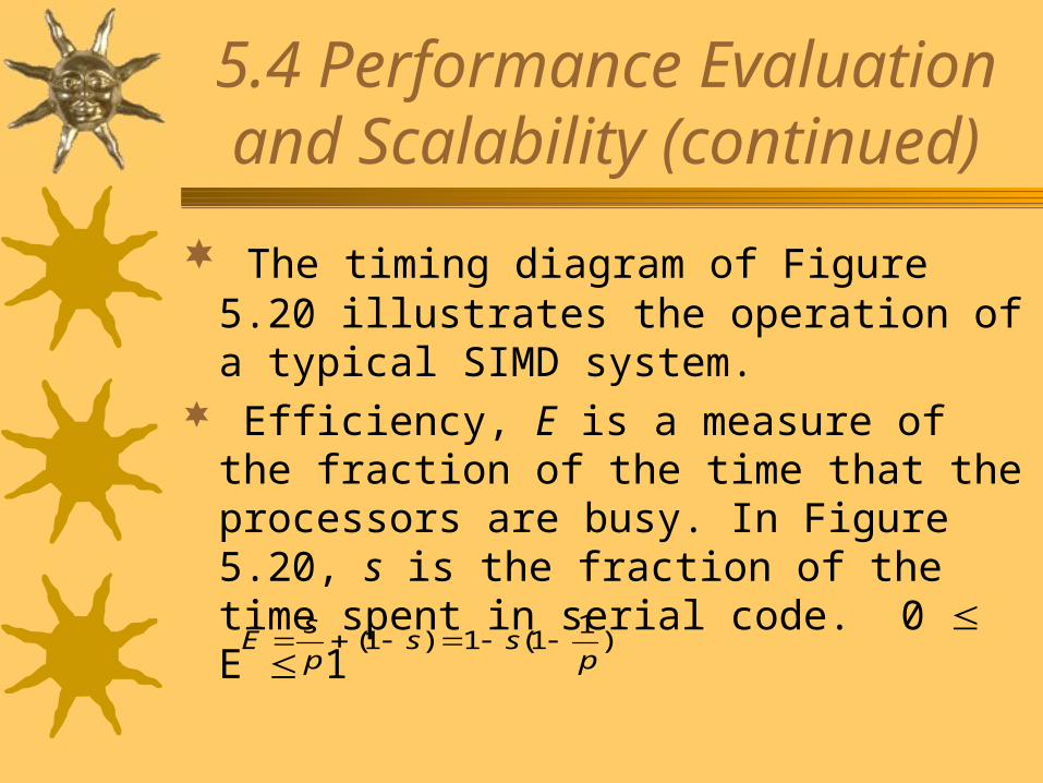
(continued) The timing diagram of Figure 5.20
illustrates the operation of a typical SIMD system.
Efficiency, E is a measure of the fraction of the time that the processors are busy. In Figure 5.20, s is the fraction of the time spent in serial code. 0 E 1
)1
1(1)1(p
ssp
sE
5.4 Performance Evaluation and Scalability
(continued) The serial execution time in
Figure 5.20 is one unit and if the code that can be run in parallel takes N time units on a single processor system,
The efficiency is also defines as
Np
p
pN
s
1
1
p
SE

5.4 Performance Evaluation and Scalability
(continued)The cost is the product of the
parallel run time and the number of processors. – Cost optimal: if the cost of a parallel
system is proportional to the execution time of the fastest algorithm.
Scalability is a measure of its ability to increase speedup as the number of processors increases.
5.5 Programming SIMDs
The SIMD instruction set contains additional instruction for IN operations, manipulating local and global registers, setting activity bits based on data conditions.
Popular high-level languages such as FORTRAN, C, and LISP have been extended to allow data-parallel programming on SIMDs.

5.6 Example Systems
ILLIAC-IV– The ILLIAC-IV project was started in 1966
at the University of Illinois.– A system with 256 processors controlled
by a CP was envisioned.– The set of processors was divided into four
quadrants of 64 processors.– Figure 5.21 shows the system structure.– Figure 5.22 shows the configuration of a
quadrant.– The PE array is arranged as an 8x8 torus.
5.6 Example Systems (continued)
CM-2– The CM-2, introduced in 1987, is a
massively parallel SIMD machine.– Table 5.1 summarizes its
characteristics.– Figure 5.23 shows the architecture of
CM-2.

5.6 Example Systems (continued)
CM-2– Processors
• The 16 processors are connected by a 4x4 mesh. (Figure 5.24)
• Figure 5.25 shows a processing cell.
– Hypercube• The processors are linked by a 12-dimensional
hypercube router network.• The following parallel communication operations
permit elements of parallel variables: reduce & broadcast, grid(NEWS), general(send, get), scan, spread, sort.
5.6 Example Systems (continued)
CM-2– Nexus
• A 4x4 crosspoint switch,
– Router• It is used to transmit data from a
processor to the other.
– NEWS Grid• A two-dimensional mesh that allows
nearest-neighbor communication.
5.6 Example Systems (continued)
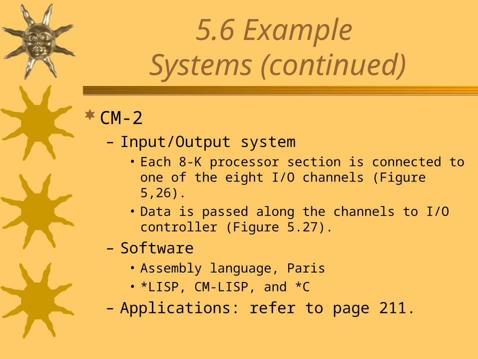
CM-2– Input/Output system
• Each 8-K processor section is connected to one of the eight I/O channels (Figure 5,26).
• Data is passed along the channels to I/O controller (Figure 5.27).
– Software• Assembly language, Paris• *LISP, CM-LISP, and *C
– Applications: refer to page 211.

5.6 Example Systems (continued)
MasPar MP– The MasPar MP-1 is a data parallel SIMD with
basic configuration consisting of the data parallel unit(DDP) and a host workstation.
– The DDP consists of from 1,024 to 16,384 processing elements.
– The programming environment is UNIX-based. Programming languages are MDF(MasPar FORTRAN), MPL(MasPar Programming Language)
5.6 Example Systems (continued)
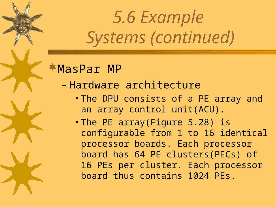
MasPar MP– Hardware architecture
• The DPU consists of a PE array and an array control unit(ACU).
• The PE array(Figure 5.28) is configurable from 1 to 16 identical processor boards. Each processor board has 64 PE clusters(PECs) of 16 PEs per cluster. Each processor board thus contains 1024 PEs.
5.7 Systolic Arrays
A systolic array is a special purpose planar array of simple processors that feature a regular, near-neighbor interconnection network.
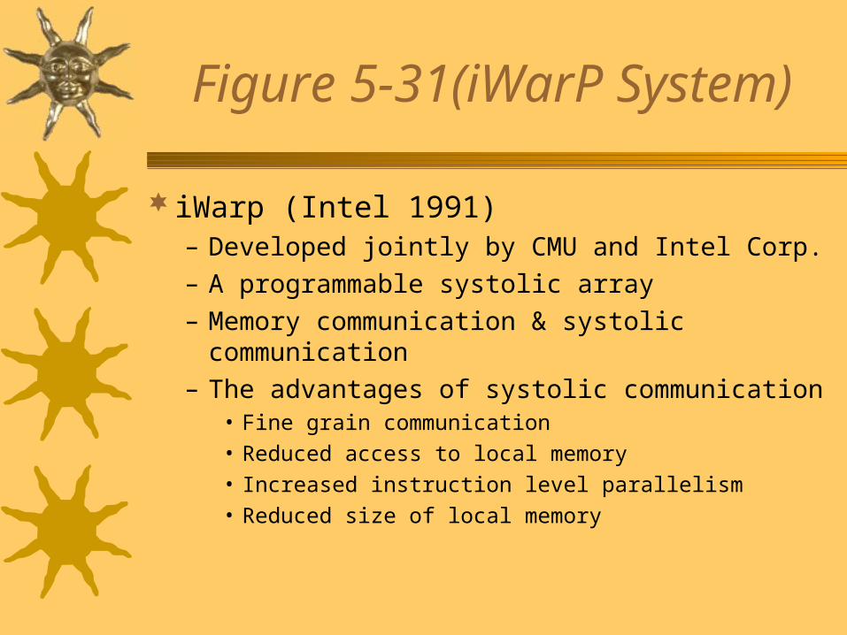
Figure 5-31(iWarP System)
iWarp (Intel 1991)– Developed jointly by CMU and Intel Corp.– A programmable systolic array– Memory communication & systolic
communication– The advantages of systolic communication
• Fine grain communication• Reduced access to local memory• Increased instruction level parallelism• Reduced size of local memory
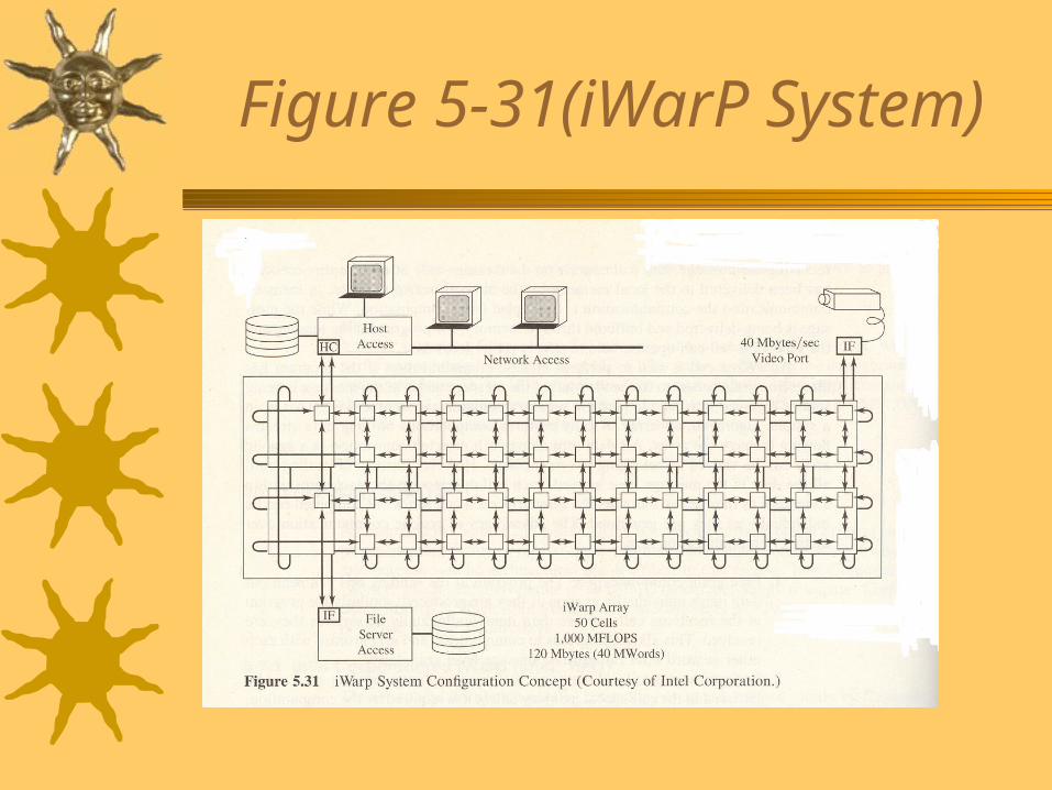
Figure 5-31(iWarP System)

Figure 5-31(iWarP System)
An iWarp system is made of an array of iWarp cells
Each iWarp cell consists of an iWarp component and the local memory.
The iWarp component contains independent communication and computation agents

Figure 5-31(iWarP System)