CHAPTER 4: RESULT

60

CHAPTER 4: RESULT

4.1: GENETIC AMPLIFICATION

All the DNA were successfully extracted using AxyPrepTM Genomic DNA

Extraction Kit (AxyPrepTM Genomic DNA Extraction Kit website:

http://www.axygenbio.com/collections/vendors?page=2&q=Axygen) and shows high

purity of DNA with optical density (OD260/280nm) ratio ranged from 1.78 to 1.84 through

spectrophotometric measurement of UV absorbance using a spectrophotometer (Eppendorf,

Germany). All the samples included in genetic analysis shows 100% successful

amplification by universal Fish F1 and Fish R1 primer set (Ward et al., 2005) with

optimum annealing temperature of 45°C and optimum amount of 25mM MgCl2 of 2µl per

reaction volume. The success of amplified COI sequence was visualized through UV gel

imaging after 1% agarose gel electrophoresis and is shown in Appendix E. These

successful amplified COI sequences were trimmed at both ends and resulted in a total

length of 582 base pair amplicon for subsequent analysis.

CHAPTER 4: RESULT

61

4.2: DNA BARCODING

A partial fragment of mtDNA COI sequence consists of a total length of 582 base

pair was generated in this study for a total of 126 barcoding specimens from 27 previously

described freshwater fish species. These COI sequences were aligned with COI sequence

in Genbank database and shows the absence of indels and in-frame stop codons which

indicate that our entire datasets were free from existence of nuclear mitochondrial

pseudogenes (numts). Hence, it is assumed that our COI barcodes are functional

mitochondrial COI sequence and therefore were suitable for subsequent data analysis.

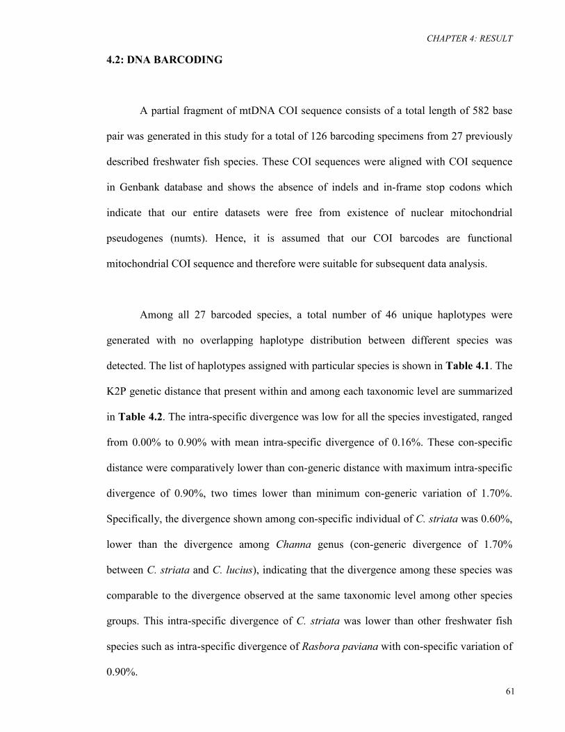
Among all 27 barcoded species, a total number of 46 unique haplotypes were

generated with no overlapping haplotype distribution between different species was

detected. The list of haplotypes assigned with particular species is shown in Table 4.1. The

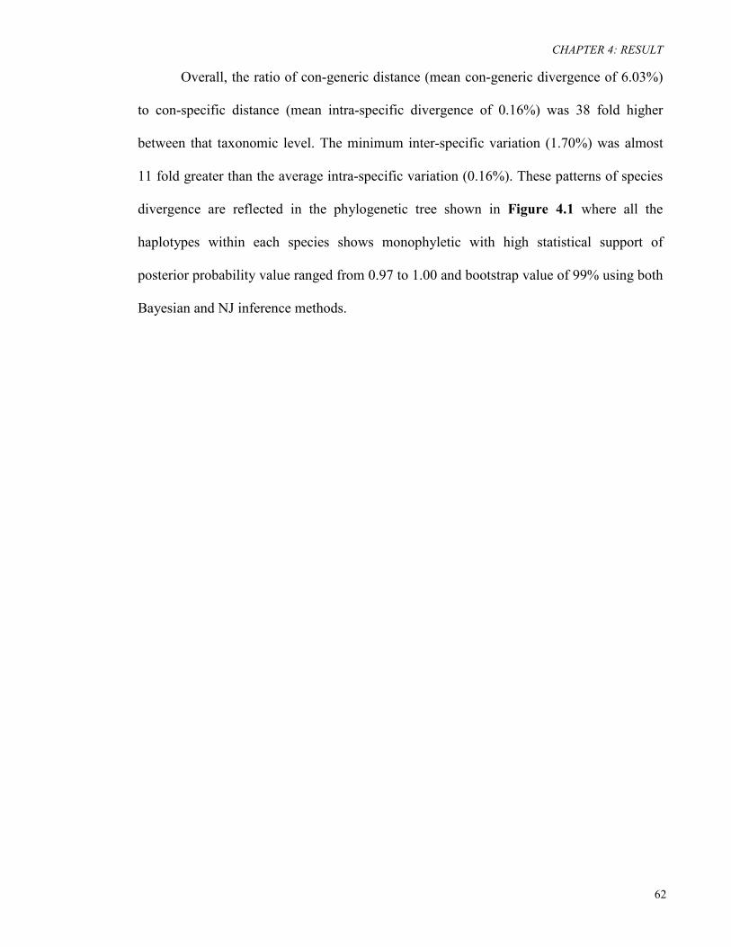
K2P genetic distance that present within and among each taxonomic level are summarized

in Table 4.2. The intra-specific divergence was low for all the species investigated, ranged

from 0.00% to 0.90% with mean intra-specific divergence of 0.16%. These con-specific

distance were comparatively lower than con-generic distance with maximum intra-specific

divergence of 0.90%, two times lower than minimum con-generic variation of 1.70%.

Specifically, the divergence shown among con-specific individual of C. striata was 0.60%,

lower than the divergence among Channa genus (con-generic divergence of 1.70%

between C. striata and C. lucius), indicating that the divergence among these species was

comparable to the divergence observed at the same taxonomic level among other species

groups. This intra-specific divergence of C. striata was lower than other freshwater fish

species such as intra-specific divergence of Rasbora paviana with con-specific variation of

0.90%.

CHAPTER 4: RESULT

62

Overall, the ratio of con-generic distance (mean con-generic divergence of 6.03%)

to con-specific distance (mean intra-specific divergence of 0.16%) was 38 fold higher

between that taxonomic level. The minimum inter-specific variation (1.70%) was almost

11 fold greater than the average intra-specific variation (0.16%). These patterns of species

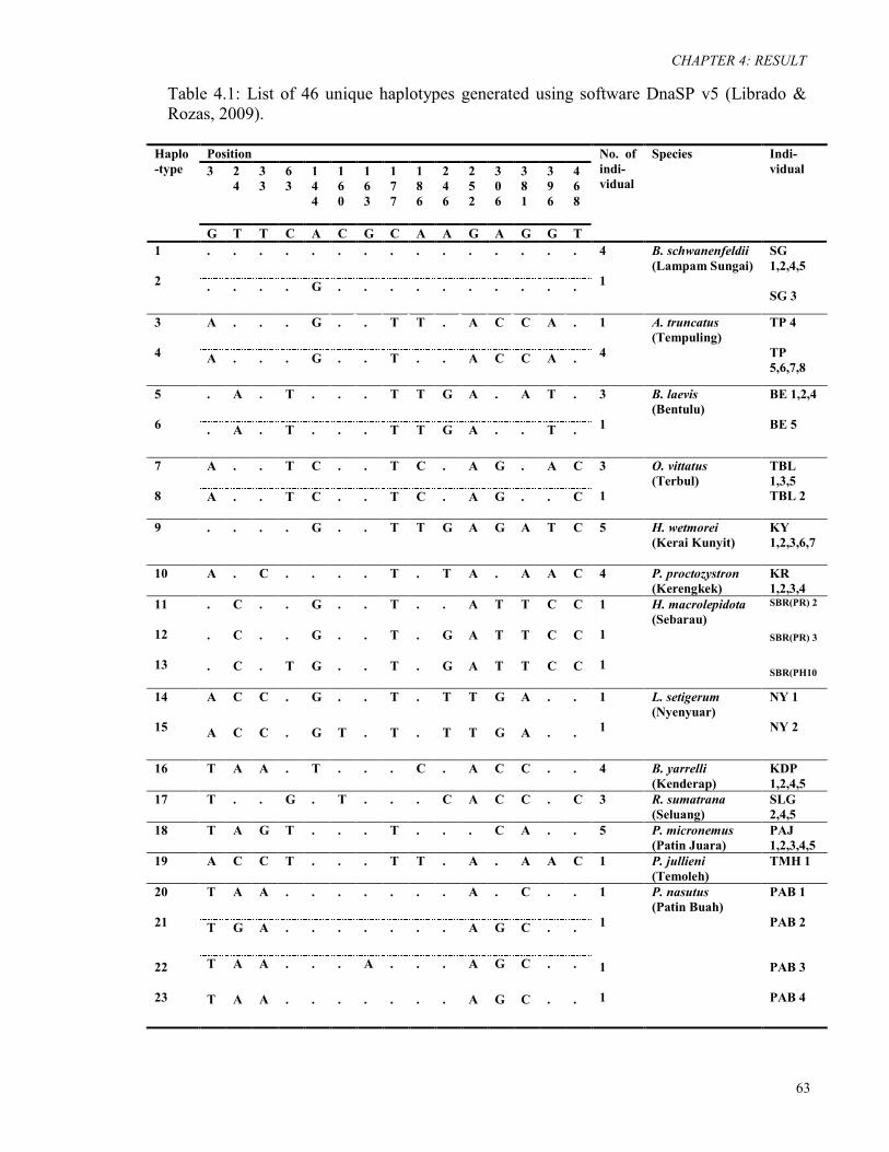
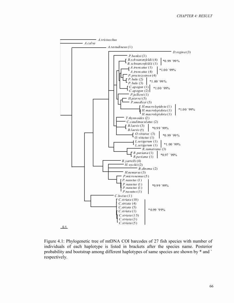
divergence are reflected in the phylogenetic tree shown in Figure 4.1 where all the

haplotypes within each species shows monophyletic with high statistical support of

posterior probability value ranged from 0.97 to 1.00 and bootstrap value of 99% using both

Bayesian and NJ inference methods.

CHAPTER 4: RESULT

63

Table 4.1: List of 46 unique haplotypes generated using software DnaSP v5 (Librado & Rozas, 2009).

Haplo-type

Position No. of indi- vidual

Species Indi- vidual 3 2

4 3 3

6 3

144

160

1 6 3

1 7 7

186

2 4 6

2 5 2

3 0 6

381

396

4 6 8

G T T C A C G C A A G A G G T 1 2

. . . . . . . . . . . . . . .

4 1

B. schwanenfeldii (Lampam Sungai)

SG 1,2,4,5 SG 3

. . . . G . . . . . . . . . .

3 4

A . . . G . . T T . A C C A .

1 4

A. truncatus (Tempuling)

TP 4 TP 5,6,7,8

A . . . G . . T . . A C C A .

5 6

. A . T . . . T T G A . A T .

3 1

B. laevis (Bentulu)

BE 1,2,4 BE 5 . A . T . . . T T G A . . T .

7 8

A . . T C . . T C . A G . A C

3 1

O. vittatus (Terbul)

TBL 1,3,5 TBL 2 A . . T C . . T C . A G . . C

9 . . . . G . . T T G A G A T C 5

H. wetmorei (Kerai Kunyit)

KY 1,2,3,6,7

10 A . C . . . . T . T A . A A C 4 P. proctozystron (Kerengkek)

KR 1,2,3,4

11 12 13

. C . . G . . T . . A T T C C

1 1 1

H. macrolepidota (Sebarau)

SBR(PR) 2 SBR(PR) 3 SBR(PH10

. C . . G . . T . G A T T C C

. C . T G . . T . G A T T C C

14 15

A C C . G . . T . T T G A . .

1 1

L. setigerum (Nyenyuar)

NY 1 NY 2 A C C . G T . T . T T G A . .

16 T A A . T . . . C . A C C . . 4 B. yarrelli

(Kenderap) KDP 1,2,4,5

17 T . . G . T . . . C A C C . C 3 R. sumatrana (Seluang)

SLG 2,4,5

18 T A G T . . . T . . . C A . . 5 P. micronemus (Patin Juara)

PAJ 1,2,3,4,5

19 A C C T . . . T T . A . A A C 1 P. jullieni (Temoleh)

TMH 1

20 21 22 23

T A A . . . . . . . A . C . .

1 1 1 1

P. nasutus (Patin Buah)

PAB 1 PAB 2 PAB 3 PAB 4

T G A . . . . . . . A G C . .

T A A . . . A . . . A G C . .

T A A . . . . . . . A G C . .

CHAPTER 4: RESULT

64

Table continued’

Haplo-type

Position No. of indi- vidual

Species Indi- vidual 3 2

4 3 3

6 3

144

160

1 6 3

1 7 7

186

2 4 6

252

3 0 6

381

396

468

G T T C A C G C A A G A G G T 24 . . C . . . . T . G A . A . . 2 T. thynnoides

(Lomah) LMH 1,2

25 T A A . . . . T . . A C A . . 2 H. wyckii (Baung Kelulang)

BAK 1,2

26 A . . T . . . . . C C T A . .

2 C. caudimaculatus (Selimang Batu)

SLB 1,2

27 28

A . . T G . . T . T . . A . C

1 2

C.apogon (Temperas)

TEM 2 TEM 3,5 A . . . G . . T . T . . A A C

29 . A . T . . . T . C C C T T . 1 A. testudineus

(Puyu) PY 1

30 T A . . . . . . C T T G C A C 2 B.dinema (Gerahak)

GER 1,2

31 32

A . . . . G . T . . A . A . C

2 3

P.bulu (Tengalan)

TGL 1,5 TGL 2,3,4 A . . . . G . T G . A . A . C

33 34 35 36 37 38 39

. A A A . . . . C C . . . . . 10 6 3 4 5 5 1

C.striata (Haruan)

HRN(JH)8,11,15,25,30 & HRN (NS)6,11,13,14,15 HRN(PP)1,4&HRN(KD)1-4&HRN(SRW)1, 3-10 HRN(PP) 2,3,6 HRN(TG) 5,6,8,16 HRN(PH)6,7,9,10,12 HRN(SL) 16,18,20,26,27 HRN(SRW)2

. A A A . . . . C G A . . . .

. A A A . . . T C G A . . . .

. A A A . . . T C C A . . . .

. A A A . . . . C C A G . . .

. A G A . . . . C G A . . . .

. A A A . . . . C C A . . . .

40 41

T C . G G T . . . C A G A . . 1 1

R.paviana (Seluang)

SLG(PR) 1 SLG(SL) 1 T C . G G T . . . C A G A . C

42

T A A . . . . T . . A . A A . 3

H.nemurus (Baung)

BAU(PR) 1,2,3

43 A G . . G . . T . G A C T A . 3 D.regina (Danio)

DNO(PR) 1,2,3

44 A . G . G . . . . T A C C A . 1 C.lucius (Bujuk)

BJK(PR) 1

45 A . . T . . T T . A . C A C

3 P. banksi (Tengas)

PBA(SL) 1,2,3

46 A . . T . . . . G A . . T . 5 P. smedleyi (Tengas Daun)

TGSD(SL) 2,3,4,10,11

CHAPTER 4: RESULT

65

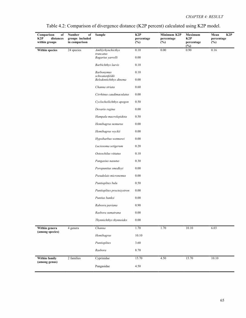
Table 4.2: Comparison of divergence distance (K2P percent) calculated using K2P model.

Comparison of K2P distances within groups

Number of groups included in comparison

Sample K2P percentage (%)

Minimum K2P percentage (%)

Maximum K2P percentage (%)

Mean K2P percentage (%)

Within species

24 species

Amblyrhynchicthys truncatus

0.10 0.00 0.90 0.16

Bagarius yarrelli

0.00

Barbichthys laevis

0.10

Barbonymus schwanenfeldii

0.10

Belodontichthys dinema

0.00

Channa striata

0.60

Cirrhinus caudimaculatus

0.00

Cyclocheilichthys apogon

0.50

Devario regina

0.00

Hampala macrolepidota

0.50

Hemibagrus nemurus

0.00

Hemibagrus wyckii

0.00

Hypsibarbus wetmorei

0.00

Luciosoma setigerum

0.20

Osteochilus vittatus

0.10

Pangasius nasutus

0.30

Poropuntius smedleyi

0.00

Pseudolais micronemus

0.00

Puntioplites bulu

0.50

Puntioplites proctozystron

0.00

Puntius banksi

0.00

Rabosra paviana

0.90

Rasbora sumatrana

0.00

Thynnichthys thynnoides

0.00

Within genera (among species)

4 genera Channa 1.70 1.70 10.10 6.03

Hemibagrus 10.10

Puntioplites 3.60

Rasbora

8.70

Within family (among genus)

2 families

Cyprinidae 15.70 4.50 15.70 10.10

Pangasidae 4.50

CHAPTER 4: RESULT

66

0.1

A.tris toechusA.calva

A.tes tudineus (1 )

D.regina (3)P.banksi (3 )B.schwanen feldii (4)B. schwanenfeld ii (1)A .truncatus (1)A .truncatus (4)

P.proctozystron (4)P.bulu (2)P.bulu (3)C.apogon (1)C.apogon (2)P.ju llieni (1)

H.pierrei (5)P.smedleyi (5)

H.macro lepido ta (1 )H.macrolepidota (1)H.macrolepidota (1)

T.thynnoides (2 )C.caud imaculatus (2)B.laevis (3)B.laevis (1)

O.vit tatus (3)O.vi tta tus (1)L.set igerum (1)L.set igerum (1)

R. sumatrana (3)R .paviana (1)R.paviana (1)

B .yarrelli (4)H.wycki i (2)

B .dinema (2)H.nemurus (3)P.micronemus (5 )P.nasu tus (1 )P.nasu tus (1 )P.nasu tus (1 )P.nasutus (1)

C.lucius (1 )C.striata (10 )C.striata (4)C.striata (5)C.striata (1)C.stria ta (15)C.stria ta (3 )C.stria ta (5 )

*0 .99 `99%

*1.00 `99%

*1 .00 `99 %

*1.00 `99%

*1.00 `99%

*0.9 9 `99%

*0 .99 `99%

*1. 00 `99%

*0.97 `99%

*0.9 9 `99%

* 0.99 9̀ 9%

Figure 4.1: Phylogenetic tree of mtDNA COI barcodes of 27 fish species with number of individuals of each haplotype is listed in brackets after the species name. Posterior probability and bootstrap among different haplotypes of same species are shown by * and ` respectively.

CHAPTER 4: RESULT

67

4.3: MOLECULAR DATA (COI) OF C.striata

A total of 43 C. striata individuals were molecularly surveyed in this study and

were characterized with a total length of 582 base pair of mtDNA COI partial fragment.

These sequenced C. striata specimens were barcoded during barcoding analysis and all

these 43 C. striata barcodes showed 0.60% of intra-species divergence strongly indicates

that variation was present among C. striata populations surveyed in this study and thus

these COI barcodes are suitable for subsequent genetic analysis at population level. Among

the entire COI sequence obtained, a total of nine polymorphic sites had been detected with

the overall nucleoside diversity of 1.55%. All the nine variable sites are parsimony

informative. There are a total of seven haplotypes identified from all the C. striata

populations investigated in molecular study and with the haplotype diversity value of h =

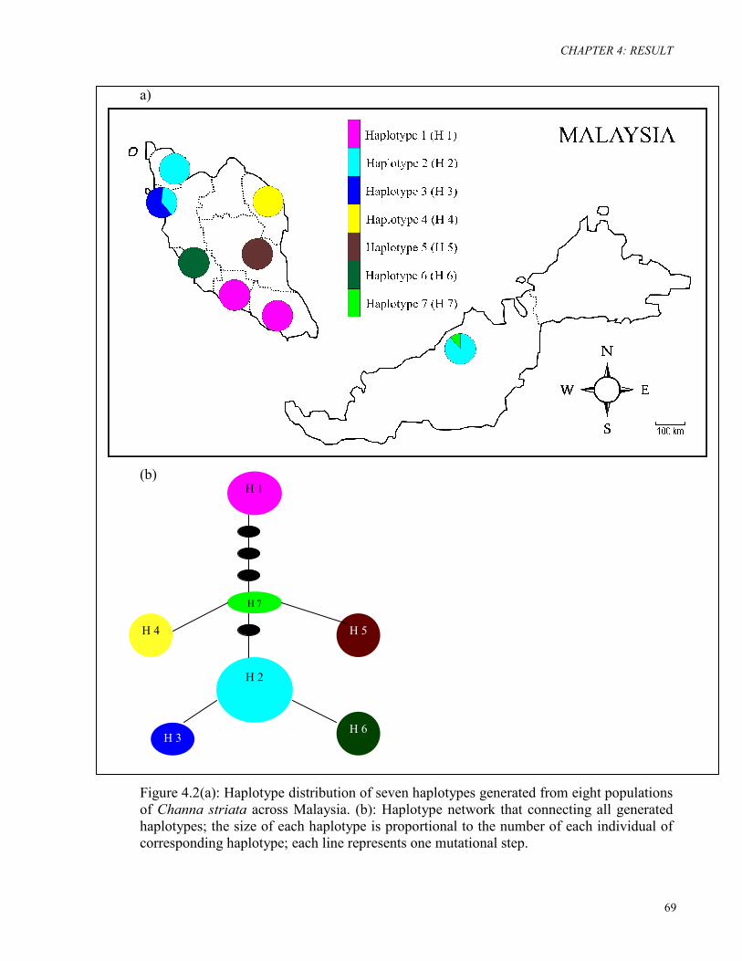
0.8018 being recorded. Among all seven generated haplotypes (hap), hap2 was the most

common haplotype and was shared among populations in Kedah, Pulau Pinang and

unexpectedly, in the island of Borneo, Sarawak. Populations in the central coast of

Peninsular Malaysia were characterized by a unique haplotype; hap6, hap5, and hap4

which are specific to Selangor, Pahang, and Terengganu respectively. The haplotype

distribution pattern in Peninsular Malaysia was parallel to the freshwater fish division

proposed by Mohsin & Ambak (1983, 1991) witnessed by the overlapping haplotype

laterally between populations within the north and between populations within the south

coast, with the exception of non-overlapping haplotype within the central coast. Refer

Figure 4.2 for illustration map of haplotype distribution of C. striata across Malaysia.

CHAPTER 4: RESULT

68

The populations structure of C. striata were explained by the obtained mtDNA COI

Fst values with the p < 0.05 as the cut off point of significant population differentiation.

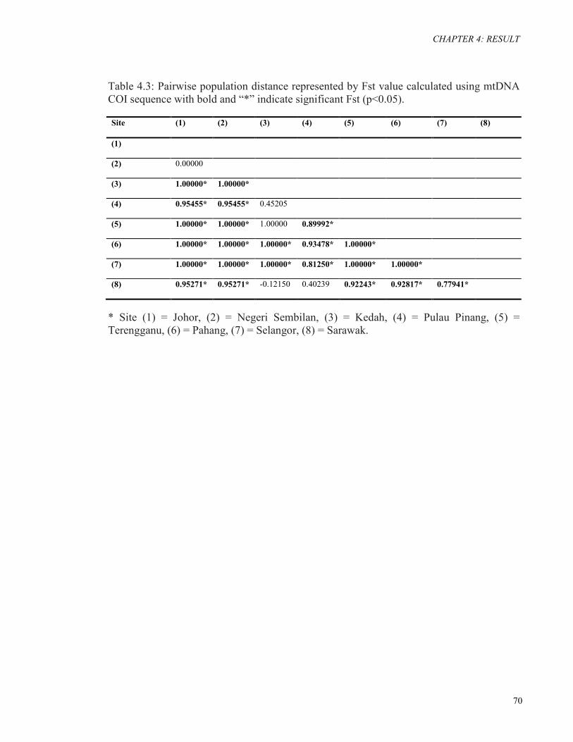
This population differentiation is summarized in Table 4.3. All the populations in

Peninsular Malaysia were significantly differentiated with each other except populations

which are separated in short distance, such as between Kedah and Pulau Pinang, between

Kedah and Terengganu, and between Negeri Sembilan and Johor. Among the entire C.

striata populations in Malaysia, an interesting result is the non-significant population

differentiation between West Malaysia (Kedah and Pulau Pinang) and East Malaysia

(Sarawak). This interesting finding coupled with the evidence of sharing of hap2 was an

unexpected genetically incomplete population divergence between the Peninsular Malaysia

and the island of Borneo which are geographically isolated by recent physical barrier of

South China Sea.

CHAPTER 4: RESULT

69

a) (b) Figure 4.2(a): Haplotype distribution of seven haplotypes generated from eight populations of Channa striata across Malaysia. (b): Haplotype network that connecting all generated haplotypes; the size of each haplotype is proportional to the number of each individual of corresponding haplotype; each line represents one mutational step.

H 7

H 2

H 3 H 6

H 4 H 5

H 1

CHAPTER 4: RESULT

70

Table 4.3: Pairwise population distance represented by Fst value calculated using mtDNA COI sequence with bold and “*” indicate significant Fst (p<0.05). Site (1)

(2)

(3)

(4)

(5)

(6)

(7)

(8)

(1)

(2)

0.00000

(3)

1.00000* 1.00000*

(4)

0.95455* 0.95455* 0.45205

(5)

1.00000* 1.00000* 1.00000 0.89992*

(6)

1.00000* 1.00000* 1.00000* 0.93478* 1.00000*

(7)

1.00000* 1.00000* 1.00000* 0.81250* 1.00000* 1.00000*

(8)

0.95271* 0.95271* -0.12150 0.40239 0.92243* 0.92817* 0.77941*

* Site (1) = Johor, (2) = Negeri Sembilan, (3) = Kedah, (4) = Pulau Pinang, (5) = Terengganu, (6) = Pahang, (7) = Selangor, (8) = Sarawak.

CHAPTER 4: RESULT

71

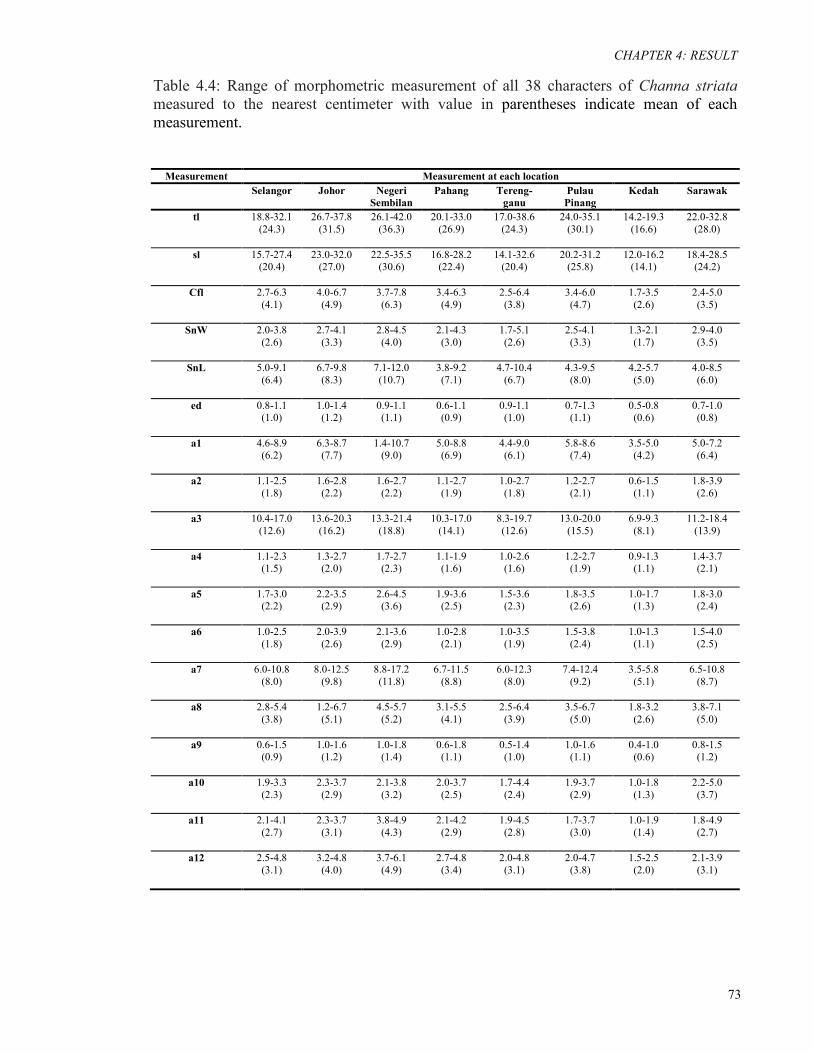
4.4: MORPHOMETRIC DATA OF C. striata

A total of 38 morphometric measurements (refer Table 4.4) were obtained for all C.

striata individuals sampled in this study and the 30 successfully transformed variables

were able to discriminate populations of C. striata in Malaysia. These patterns of

discrimination were illustrated in differents root represented in two-dimensional graph in

Figure 4.3 and Figure 4.4 with the zero cut off point in each root acted as a dividing point

in discriminating populations from positive region which acquired certain unique

characters in relation to other populations in negative region at the same root. A list of

standardized coefficients of canonical variables underlying unique characters that could

discriminate certain populations from others was generated (Table 4.5 and Table 4.6)

which acted as a reference for its correspondence two-dimensional graph. The eigenvalue

under each root for each list was calculated representing the amount of variation that each

root can explained and the value of cumulative proportion for each root was demonstrating

the percentage of variation accounted by each root among all the roots. The two characters

that had greatest contribution of variance to each root were represented in Table 4.5 and

Table 4.6 whereby these characters were with the two tops value of coefficient under each

root.

CHAPTER 4: RESULT

72

The first stage of multivariate discriminant analysis for the populations in

Peninsular Malaysia is illustrated in the discriminant graph shown in Figure 4.3. For the C.

striata populations surveyed in Peninsular Malaysia, there are four distinct groups had

been discovered; there are: group A (Selangor, Pahang and Terengganu), group B (Johor,

Pulau Pinang), group C (Negeri Sembilan) and group D (Kedah). These four groups are

distinguishable from each other based on the obtained 30 successfully transformed

morphometric measurements. The major components of variance which discriminate

between the groups was underlined by root 1 axis followed by root 2 axis which contribute

to percentage of variation of 58.54% and 18.49% respectively. The greatest contribution of

characters that discriminated by root 1 axis were measurements of c2 and e1; whereas the

most discriminant characters on root 2 axis were measurements of c3 and d2. Refer Table

4.5 for the percentage of variance components of each axis and the most discriminated

measurements reflected by each axis. Hence, within Peninsular Malaysia, group A which

consists of populations of Selangor, Pahang and Terengganu were discriminated from

group B, C and D by unique characters of comparative small measurement of c2 trait and

large measurement of e1 trait which are the characters located on head. Similarly, group B

and C which are populations of Johor, Pulau Pinang and Negeri Sembilan were

characterized by unique head characters of small measurement of c3 trait and small

measurement of d2 trait in relation to populations from Kedah (group D).

CHAPTER 4: RESULT

73

Table 4.4: Range of morphometric measurement of all 38 characters of Channa striata measured to the nearest centimeter with value in parentheses indicate mean of each measurement.

Measurement Measurement at each location Selangor Johor Negeri

Sembilan Pahang Tereng-

ganu Pulau Pinang

Kedah Sarawak

tl 18.8-32.1 (24.3)

26.7-37.8 (31.5)

26.1-42.0 (36.3)

20.1-33.0 (26.9)

17.0-38.6 (24.3)

24.0-35.1 (30.1)

14.2-19.3 (16.6)

22.0-32.8 (28.0)

sl 15.7-27.4 (20.4)

23.0-32.0 (27.0)

22.5-35.5 (30.6)

16.8-28.2 (22.4)

14.1-32.6 (20.4)

20.2-31.2 (25.8)

12.0-16.2 (14.1)

18.4-28.5 (24.2)

Cfl 2.7-6.3 (4.1)

4.0-6.7 (4.9)

3.7-7.8 (6.3)

3.4-6.3 (4.9)

2.5-6.4 (3.8)

3.4-6.0 (4.7)

1.7-3.5 (2.6)

2.4-5.0 (3.5)

SnW 2.0-3.8 (2.6)

2.7-4.1 (3.3)

2.8-4.5 (4.0)

2.1-4.3 (3.0)

1.7-5.1 (2.6)

2.5-4.1 (3.3)

1.3-2.1 (1.7)

2.9-4.0 (3.5)

SnL 5.0-9.1 (6.4)

6.7-9.8 (8.3)

7.1-12.0 (10.7)

3.8-9.2 (7.1)

4.7-10.4 (6.7)

4.3-9.5 (8.0)

4.2-5.7 (5.0)

4.0-8.5 (6.0)

ed 0.8-1.1 (1.0)

1.0-1.4 (1.2)

0.9-1.1 (1.1)

0.6-1.1 (0.9)

0.9-1.1 (1.0)

0.7-1.3 (1.1)

0.5-0.8 (0.6)

0.7-1.0 (0.8)

a1 4.6-8.9 (6.2)

6.3-8.7 (7.7)

1.4-10.7 (9.0)

5.0-8.8 (6.9)

4.4-9.0 (6.1)

5.8-8.6 (7.4)

3.5-5.0 (4.2)

5.0-7.2 (6.4)

a2 1.1-2.5 (1.8)

1.6-2.8 (2.2)

1.6-2.7 (2.2)

1.1-2.7 (1.9)

1.0-2.7 (1.8)

1.2-2.7 (2.1)

0.6-1.5 (1.1)

1.8-3.9 (2.6)

a3 10.4-17.0 (12.6)

13.6-20.3 (16.2)

13.3-21.4 (18.8)

10.3-17.0 (14.1)

8.3-19.7 (12.6)

13.0-20.0 (15.5)

6.9-9.3 (8.1)

11.2-18.4 (13.9)

a4 1.1-2.3 (1.5)

1.3-2.7 (2.0)

1.7-2.7 (2.3)

1.1-1.9 (1.6)

1.0-2.6 (1.6)

1.2-2.7 (1.9)

0.9-1.3 (1.1)

1.4-3.7 (2.1)

a5 1.7-3.0 (2.2)

2.2-3.5 (2.9)

2.6-4.5 (3.6)

1.9-3.6 (2.5)

1.5-3.6 (2.3)

1.8-3.5 (2.6)

1.0-1.7 (1.3)

1.8-3.0 (2.4)

a6 1.0-2.5 (1.8)

2.0-3.9 (2.6)

2.1-3.6 (2.9)

1.0-2.8 (2.1)

1.0-3.5 (1.9)

1.5-3.8 (2.4)

1.0-1.3 (1.1)

1.5-4.0 (2.5)

a7

6.0-10.8 (8.0)

8.0-12.5 (9.8)

8.8-17.2 (11.8)

6.7-11.5 (8.8)

6.0-12.3 (8.0)

7.4-12.4 (9.2)

3.5-5.8 (5.1)

6.5-10.8 (8.7)

a8

2.8-5.4 (3.8)

1.2-6.7 (5.1)

4.5-5.7 (5.2)

3.1-5.5 (4.1)

2.5-6.4 (3.9)

3.5-6.7 (5.0)

1.8-3.2 (2.6)

3.8-7.1 (5.0)

a9

0.6-1.5 (0.9)

1.0-1.6 (1.2)

1.0-1.8 (1.4)

0.6-1.8 (1.1)

0.5-1.4 (1.0)

1.0-1.6 (1.1)

0.4-1.0 (0.6)

0.8-1.5 (1.2)

a10

1.9-3.3 (2.3)

2.3-3.7 (2.9)

2.1-3.8 (3.2)

2.0-3.7 (2.5)

1.7-4.4 (2.4)

1.9-3.7 (2.9)

1.0-1.8 (1.3)

2.2-5.0 (3.7)

a11

2.1-4.1 (2.7)

2.3-3.7 (3.1)

3.8-4.9 (4.3)

2.1-4.2 (2.9)

1.9-4.5 (2.8)

1.7-3.7 (3.0)

1.0-1.9 (1.4)

1.8-4.9 (2.7)

a12

2.5-4.8 (3.1)

3.2-4.8 (4.0)

3.7-6.1 (4.9)

2.7-4.8 (3.4)

2.0-4.8 (3.1)

2.0-4.7 (3.8)

1.5-2.5 (2.0)

2.1-3.9 (3.1)

CHAPTER 4: RESULT

74

Table continued’

Measurement Measurement at each location Selangor Johor Negeri

Sembilan Pahang Tereng-

ganu Pulau Pinang

Kedah Sarawak

b1

2.7-5.0 (3.4)

3.4-5.1 (4.3)

4.0-6.3 (5.4)

3.0-4.8 (3.6)

2.4-4.8 (3.3)

3.0-5.2 (4.0)

1.8-3.2 (2.6)

2.5-3.8 (3.1)

b2

2.0-3.6 (2.5)

2.1-3.8 (3.1)

3.1-4.7 (4.2)

2.3-3.8 (2.8)

1.3-3.6 (2.5)

2.0-3.7 (2.9)

1.6-2.4 (2.0)

2.0-3.0 (2.6)

b3

1.8-2.9 (2.2)

2.6-4.3 (3.3)

4.1-5.4 (4.7)

2.1-3.8 (2.8)

1.7-3.3 (2.3)

2.1-4.3 (3.2)

1.4-2.5 (2.1)

1.5-3.0 (2.6)

b4

3.5-5.6 (4.2)

5.5-7.1 (6.3)

4.7-8.2 (7.4)

2.8-5.9 (4.8)

2.0-5.6 (4.1)

4.8-7.1 (6.1)

1.9-3.6 (2.9)

3.4-6.6 (5.0)

c1

3.3-6.3 (4.3)

5.1-6.6 (5.7)

4.8-8.3 (7.4)

3.7-6.5 (5.0)

3.0-6.5 (4.4)

4.9-6.6 (5.6)

2.0-3.9 (3.0)

3.4-6.9 (4.5)

c2 2.5-4.5 (3.4)

5.4-7.0 (6.1)

4.3-8.3 (7.4)

2.5-5.9 (4.7)

2.4-4.5 (3.3)

5.2-7.0 (6.1)

2.1-4.6 (3.8)

3.0-5.3 (4.1)

c3 3.9-6.9 (4.9)

6.0-7.5 (6.6)

4.4-8.4 (7.5)

4.0-7.0 (5.8)

3.7-6.8 (4.6)

5.4-7.5 (6.5)

2.3-4.3 (3.8)

3.9-6.3 (5.2)

d1 3.2-5.2 (4.1)

6.1-8.5 (7.0)

4.5-8.8 (7.7)

3.2-6.7 (5.3)

3.1-5.2 (4.0)

5.5-8.5 (6.9)

2.4-4.5 (4.0)

2.9-5.5 (4.2)

d2 4.1-7.1 (4.9)

6.0-8.3 (6.6)

4.5-8.5 (7.5)

4.1-7.5 (6.1)

3.1-7.3 (4.9)

5.9-8.3 (6.7)

2.9-4.7 (4.0)

2.8-5.0 (4.1)

e1

3.7-6.1 (4.6)

6.1-9.0 (7.5)

4.7-9.3 (8.1)

4.2-7.6 (6.3)

3.8-5.9 (4.7)

5.4-9.0 (7.3)

3.0-4.8 (4.2)

3.4-5.6 (4.7)

e2 4.1-7.8 (5.3)

6.0-8.6 (6.9)

4.0-9.2 (7.8)

4.4-8.0 (6.6)

3.8-7.0 (5.2)

5.3-8.6 (6.8)

2.8-4.3 (3.6)

3.0-4.7 (4.0)

f1 5.4-9.4 (6.8)

7.8-11.3 (8.8)

7.5-10.8 (10.1)

5.7-8.9 (7.8)

5.0-8.9 (6.6)

7.0-11.3 (8.9)

2.9-5.2 (4.4)

4.6-7.8 (6.2)

f2 7.1-12.5 (9.3)

10.1-13.3 (11.3)

10.7-15.5 (14.6)

7.1-12.0 (10.3)

6.8-12.5 (8.9)

9.1-13.3 (11.1)

3.9-6.6 (5.6)

7.2-12.0 (9.4)

g1

9.4-17.3 (12.5)

14.1-18.0 (15.7)

14.4-20.6 (19.3)

10.4-15.5 (13.8)

4.0-16.4 (12.1)

13.2-18.0 (15.4)

6.8-9.3 (8.4)

9.4-15.5 (13.3)

g2 2.1-4.1 (2.7)

3.1-4.7 (3.7)

3.4-4.6 (4.0)

2.1-4.0 (3.3)

1.9-3.9 (2.6)

2.9-4.7 (3.5)

1.0-2.2 (1.7)

1.5-3.4 (2.7)

g3 2.3-4.0 (3.0)

3.0-4.9 (3.9)

3.5-5.5 (4.7)

2.3-4.4 (3.5)

2.1-4.0 (2.9)

2.7-4.9 (3.7)

1.2-2.8 (2.2)

2.1-4.5 (3.4)

g4 2.1-3.7 (2.6)

3.0-4.6 (3.5)

3.2-4.8 (4.2)

2.1-3.9 (3.1)

1.9-3.5 (2.7)

2.5-4.6 (3.4)

1.6-2.5 (2.1)

2.2-4.0 (3.1)

h1

2.6-4.7 (3.6)

4.0-5.7 (4.8)

3.8-6.4 (5.5)

3.1-4.8 (4.2)

2.8-4.7 (3.6)

3.9-5.7 (4.7)

1.4-2.8 (2.3)

2.8-5.0 (4.1)

h2

4.1-8.0 (5.7)

5.7-8.3 (7.2)

6.1-9.6 (8.8)

5.0-7.4 (6.4)

3.7-8.0 (5.6)

5.6-8.2 (7.0)

3.5-4.8 (4.3)

3.2-5.7 (4.7)

h3

1.5-3.0 (2.0)

2.1-2.9 (2.5)

2.5-3.5 (3.3)

1.3-3.1 (2.2)

1.3-3.3 (2.1)

1.5-2.9 (2.4)

1.3-1.8 (1.5)

1.5-2.5 (1.9)

CHAPTER 4: RESULT

75

���� � ��� ���� ���� �������������������� ��� ���������� ������� �� �� �� �� � � � � � ������ ���������

�������� !"

Figure 4.3: Multivariate discriminant analysis represented by root 1 and root 2 axis based on all Channa striata populations surveyed in Peninsular Malaysia.

Group A Group B

Group C

Group D

CHAPTER 4: RESULT

76

Table 4.5: List of standardized coefficients of canonical variables based on all Channa striata populations surveyed in Peninsular Malaysia. Measurements in “bold” and “underline” indicate greatest contribution of characters to each root. The variables are corresponding toTruss Network Measurement illustrated in Figure 3.2.

Variable Standardized Coefficients for Canonical Variables

Root 1 Root 2 Root 3 Root 4 Root 5 Root 6 c2 -1.41184 0.499825 0.398591 0.054463 0.119042 -0.238883 f2 0.47170 0.408845 -0.615390 -0.168215 -0.230770 -0.211542 b2 0.28101 -0.278591 -0.284479 0.174256 -0.42253 0.458817 a10 0.41539 0.096533 -0.367550 -0.432404 0.259111 -0.268992 c3 0.66377 -0.858751 0.014077 0.472265 -0.250660 -0.080690 a5 0.36065 0.314906 -0.225384 -0.008893 0.267024 0.198322 e2 0.37393 0.331761 -0.266962 0.681100 -0.058005 -0.360663 b4 -0.19458 0.132053 0.252415 -0.497241 -0.523356 0.359599 SnL -0.40295 -0.046967 0.003316 -0.148526 0.532470 -0.133889 b3 -0.47636 0.368229 -0.728886 0.429959 0.008980 -0.328389 a8 0.08207 -0.149248 0.373287 -0.265477 0.015430 -0.064601 b1 -0.43399 -0.523266 -0.084456 -0.507840 -0.286558 -0.003799

SnW 0.04462 0.228839 0.184555 0.652408 -0.226785 -0.053505 e1 0.67757 -0.152426 0.587134 0.740656 0.442494 0.845807 d1 -0.46682 0.329635 0.231088 -0.655794 -0.133296 -0.085119 g2 0.43378 -0.040481 0.309560 0.4676630 -0.394074 0.556584 g4 -0.40523 -0.077577 0.026801 -0.205765 0.396488 0.091170 h2 -0.48672 0.340375 -0.166280 0.050386 0.055264 -0.023362 a3 0.27658 0.063105 0.280636 0.288647 0.163754 0.117652 a6 -0.25723 0.396127 0.321013 0.032397 -0.299612 0.211321 d2 0.07330 -0.585637 0.007170 -0.075163 -0.137986 -0.503075 c1 0.17793 0.309891 -0.142353 -0.043706 0.811599 -0.243137 a4 0.25777 0.062941 -0.042803 -0.302267 0.331285 -0.248307 g3 -0.25389 -0.259770 -0.346391 0.242604 -0.036979 0.115660 a12 0.03025 0.253880 0.294079 -0.172015 -0.278936 0.015935 g1 -0.20226 0.291106 -0.012690 0.010235 -0.403767 -0.146930 f1 0.14296 -0.046102 0.320983 -0.248611 0.212844 -0.372136 h3 -0.14463 -0.158514 -0.212149 -0.032284 -0.166438 0.353353 a9 0.08448 0.017800 -0.010266 -0.270678 0.233016 0.126766 tl 0.07500 -0.141272 -0.182243 0.040925 0.012208 0.065811

Eigenvalue 14.89929 4.705745 3.882054 1.482290 0.334059 0.148039 Cum. Prop

0.58540 (58.54%)

0.770291 (18.49%)

0.922818 (15.25%)

0.981058 (5.82%)

0.994183 (1.31%)

1.000000 (0.58%)

CHAPTER 4: RESULT

77

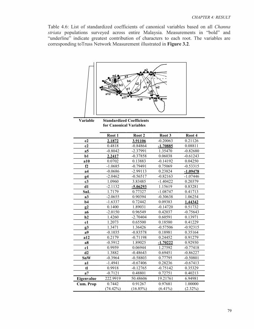
In second stage of multivariate discriminant analysis, in order to have balance

sample size, subset of each group discovered in Peninsular Malaysia together with

population from Sarawak were included in subsequent disciminant function to have a

overall discrimination on C. striata populations across entire Malaysia. This pattern f

discriminant function is shown in Figure 4.4 in which West Malaysia populations was

discriminated from East Malaysia by root 1 axis which consists of 74.42% of variance

composition in discrimination function. Populations in Peninsular Malaysia were

discriminated from the member of the island of Borneo whereby Penisula’s acquired a

comparative large measurement of e2 trait located at head and a comparative large

measurement of b1 trait located at mouth.. The degree of variance component to each axis

and the contribution of discriminant characters to each axis are shown in Table 4.6. Briefly,

populations within Peninsular Malaysia showed head polymorphism whereas populations

in Malaysia showed an additive mouth polymorphism with the evidence of large b1 trait

measurement.

CHAPTER 4: RESULT

78

#$$% & '() #$$% *+,-./012 032 0*2 0&2 2 &2 *2 32#$$% &0&40&20424

&2&4*256678

* A= Selangor, Pahang, Terengganu; B= Johor, Pulau Pinang; C= Negeri Sembilan; D= Kedah; E= Sarawak Figure 4.4: Multivariate discriminant analysis represented by root 1 and root 2 axis based on all Channa striata populations surveyed across entire Malaysia.

CHAPTER 4: RESULT

79

Table 4.6: List of standardized coefficients of canonical variables based on all Channa striata populations surveyed across entire Malaysia. Measurements in “bold” and “underline” indicate greatest contribution of characters to each root. The variables are corresponding toTruss Network Measurement illustrated in Figure 3.2.

Variable Standardized Coefficients

for Canonical Variables

Root 1 Root 2 Root 3 Root 4 e2 2.1872 3.91106 -0.20063 0.21126 c2 0.4818 -0.84864 -1.70885 0.08811 a5 -0.8042 -2.37991 1.35470 -0.82680 b1 2.2417 -0.37858 0.06038 -0.61243 a10 0.0702 0.13883 -0.14192 0.04250 f2 -1.0685 -0.79491 0.75069 -0.53315 a4 -0.0686 -2.99113 0.23824 -1.09478 g4 -2.0462 -0.56517 -0.82163 -1.07446 c3 1.0960 3.83485 -1.40422 0.20379 d1 -2.1132 -5.06293 1.15619 0.83281 SnL 1.7179 0.77327 -1.08747 0.41713 a3 -2.0655 0.90394 -0.30638 1.06254 b4 -1.6337 0.72442 0.09383 1.44342 g2 0.1400 1.89031 -0.14720 0.51732 a6 -2.0150 0.96549 0.42037 -0.75643 h2 1.4260 -2.70404 0.60591 0.13971 e1 1.2073 0.65500 0.18580 0.41229 g3 1.3471 1.36426 -0.57506 -0.92315 a9 -0.1035 -0.83578 0.18981 0.35164 a12 0.2179 -0.71198 0.24452 0.91279 a8 -0.5912 1.89025 -1.70222 0.92930 c1 0.9959 0.06944 1.27592 -0.77418 d2 1.3882 -0.48643 0.69451 -0.86227

SnW -0.3964 -0.58803 0.77795 -0.50801 a1 -1.4941 -0.67406 0.28236 -0.67413 tl 0.9918 -0.12765 -0.75142 0.35329 a7 -0.7121 0.48801 0.72751 0.40213

Eigenvalue 222.9919 50.48606 19.21761 6.94981 Cum. Prop 0.7442

(74.42%) 0.91267

(16.85%) 0.97681 (6.41%)

1.00000 (2.32%)