chapter 4 mixed farming system – an empirical...
TRANSCRIPT

Chapter 4
Mixed Farming System – An Empirical Analysis

CHAPTER 4
TABLE OF CONTENTS
Sl. No. Title Page No.
4.1 Socioeconomic Characteristics of Respondents 63
4.2 Existing Practices in Mixed Farming 68
4.3 Benefit Cost Analysis 74
4.4 Input Efficiency and Production Constraints 90
4.5 Optimum Activity Mix 110
4.6 Gender Analysis in Farming Activities 120
4.7 Conclusions 133
CHAPTER 4
MIXED FARMING SYSTEM – AN EMPIRICAL ANALYSIS
With an overview of socioeconomic characteristics of respondents and
existing practices of mixed farming system in Kerala from the data collected, this
chapter contains a detailed analysis with respect to the given objectives of the
study. There were 300 respondents from three regions in ascending order of
altitude from sea shore to mountains viz., coastal, plain and high ranges of
Palakkad and Thrissur districts of Kerala and analysis was disaggregated in terms
of region and size of farm (marginal, small and large farms). The chapter is
organized in seven parts such as (i) socioeconomic characteristics of respondents,
(ii) mixed farming practices, (iii) benefit cost ratio in mixed farming, (iv) input
efficiency and constraints, (v) optimum activity mix, (vi) gender dimensions and
(vii) conclusions.
4.1 Socioeconomic Characteristics of Respondents
The socioeconomic variables or their characteristics act as critical
determinants influencing the behaviour of respondent farmers and hence relevant
for explaining the underlying economic relations and suggesting necessary policy
measures. These characteristics are broadly classified and explained here as
demographic profile and economic features on the basis of the data pertaining to
respondents collected through field survey.
4.1.1 Demographic Profile of Respondents
The respondents surveyed in the study were 300, of which 256 were males
and 44 were females. The households surveyed for the purpose of the study had a
population of 1338 persons of which 604 were males and 734 females. Thus the
overall sex ratio stood at 1215 per 1000 men. Here it may be recalled that sex ratio
as per 2001 Census was 1058 females per 1000 males in Kerala State. The sex
ratio in high range region was high (1313) followed by coastal (1236) and plain
63

regions (1119). The other demographic features of the sample households by
caste/religion, family size, age group and level of literacy are depicted in Table 4.1.
Table 4.1. Demographic Features of Respondents (in number) Sl. No. Features Coastal Plain High range All Share to
Total (%) 1. Sex ratio 1236 1119 1313 1223 122.3
2. Religion
a. Christian 11 7 15 33 11
b. Muslim 12 5 7 24 8
c. Hindu 77 88 78 243 81
d. Hindu SC/ST 3 6 16 25 10
e. Hindu Backward
68 71 51 190 78
f. Hindu others 6 11 11 28 12
3. Family size
a. 2 – 4 40 50 64 154 51
b. 5 – 7 47 42 36 125 42
c. 8 – 10 13 8 - 21 7
4. Age group
a. 35 and below 7 2 15 24 8
b. 36 – 55 41 54 50 145 48
c. Above 55 52 44 35 131 44
5. Literacy level
a. Illiterate 4 2 20 26 9
b. Primary and Middle School
24 20 38 82 28
c. High School 52 64 38 154 51
d. Above High School
20 14 4 38 12
Source - Primary Data
64

As per Table 4.1, 243 households were Hindus constituting 81 per cent of
the total households. The distribution of households belonging to Christian and
Muslim stood at 11 and 8 percentages respectively. Of the Hindu households, the
maximum percentage share was accounted by Backward communities followed by
other caste groups and SC/ST groups. Table 4.1 also brings out the fact that the
maximum number of households (154) constituting 51 per cent belonged to the
family size group of 2 - 4. Among the surveyed farmers, 21 households had the
family size of 8 -10. The only region where the 8-10 family size was not found
belonged to high range. Taking all the regions together 48 per cent of the
respondents were in the age group of 36-55 years.
In the age group of above 55 years there were 131 respondents which
constituted 44 per cent. Thus, the surveyed regions were endowed with higher
percentage of experienced farmers. The overall literacy rate of 91 per cent for the
surveyed respondents was same as the state literacy rate of 90.92 per cent as per
2001 census. As high as 51 per cent of the respondents had high school education
while 28 per cent had educational levels of primary and middle school. Number of
persons with college and other education constituted 12 per cent of the sample.
However, it could be observed that the rate of literacy was lower in high range
region.
Followed by the demographic features, economic characteristics of the
respondents are examined in the next section.
4.1.2 Economic Features
In this section an attempt has been made to give an outline of the economic
particulars of the respondents in terms of their occupation, expenditure, land size
and average land area. Table 4.2 elucidates the details.
65
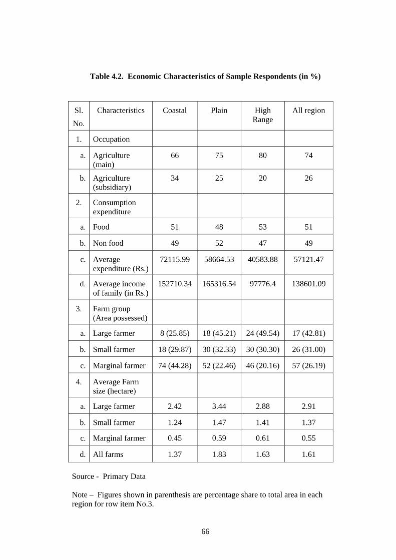
Table 4.2. Economic Characteristics of Sample Respondents (in %)
Sl.
No.
Characteristics Coastal Plain High Range
All region
1. Occupation
a. Agriculture (main)
66 75 80 74
b. Agriculture (subsidiary)
34 25 20 26
2. Consumption expenditure
a. Food 51 48 53 51
b. Non food 49 52 47 49
c. Average expenditure (Rs.)
72115.99 58664.53 40583.88 57121.47
d. Average income of family (in Rs.)
152710.34 165316.54 97776.4 138601.09
3. Farm group (Area possessed)
a. Large farmer 8 (25.85) 18 (45.21) 24 (49.54) 17 (42.81)
b. Small farmer 18 (29.87) 30 (32.33) 30 (30.30) 26 (31.00)
c. Marginal farmer 74 (44.28) 52 (22.46) 46 (20.16) 57 (26.19)
4. Average Farm size (hectare)
a. Large farmer 2.42 3.44 2.88 2.91
b. Small farmer 1.24 1.47 1.41 1.37
c. Marginal farmer 0.45 0.59 0.61 0.55
d. All farms 1.37 1.83 1.63 1.61 Source - Primary Data Note – Figures shown in parenthesis are percentage share to total area in each region for row item No.3.
66
According to Table 4.2, 74 per cent of the respondents, had farming as the
only occupation while 26 per cent had more than one occupation making farming
as subsidiary.
Average annual consumption expenditure for the sample was Rs.57121.47.
Major items of expenditure were bifurcated into food and nonfood. Region wise
and size wise expenditure pattern in detail under seven items are given separately
in Annexure-IV. The data show that the expenditure on food was more than any
other items in all the three regions, i.e., 51 per cent, 48 per cent and 53 per cent for
coastal, plain and high range, respectively. It is evident from Annexure-IV that in
plain and high range region, the percentage of expenditure on food decreased as
the size of land holdings increased. However, the total annual expenditure
increased with the increasing size of landholdings in the three regions as well as
the three size groups.
Average annual income of family for the sample was Rs.138601.09.
Average income of family was more in plain region followed by coastal and high
range. However, expenditure was more in coastal region followed by plain and
high range.
The Table 4.2 brings out the fact that in plain region 52 per cent of the
farmers were marginal farmers having less than one hectare with an average size of
farm as 0.59 hectare. In coastal regions 74 per cent were coming under marginal
farm having an average size of 0.45 hectare while in high range region 46 per cent
were marginal farmers having 0.61 hectare average size of farms. It is obvious
from the Table 4.2 that among the surveyed households in all the regions 57 per
cent of cultivating households were marginal farmers on an average having a farm
size of 0.55 hectare.
It can also be observed that large farmers who were only 17 per cent
occupied 43 per cent of areas and small farmers who were 26 per cent had 31 per
cent area. Marginal farmers (57%) possessed relatively less share (26.19%) of total
area.
67

By examining the demographic features and economic characteristics, it
can be concluded from section 4.1 that almost all (91%) were literate with a
modest family size (2-4) and active age group (36-55 years). In our sample, 74 per
cent of the respondents had agriculture as the main occupation and 83 per cent
were small and marginal farmers. Agriculture as the main occupation with small
size of holding points out the necessity of making the enterprise highly productive
for a dependable livelihood. Though the respondents were not below poverty level
as per government norms, lion’s share of expenses for food showed low income
status with lower share of income available for education, health and productive
investments. Again this points out the necessity of improvements in their
economic activity for steady and sustainable standards of living.
4.2 Existing Practices in Mixed Farming
Analysis of current practices in mixed farming in Kerala is one of the
objectives of the study. Though mixed farming has definite definitions, the
components of farming and their share may differ from region to region. In the
study area, farming was basically constituted by paddy, coconut, homestead and
dairying. The distribution of farmers according to the area utilized for various
types of farming operations and number of milch animals possessed are presented
in region and farm size wise in Table 4.3. Since no respondent is hailed from
paddy alone farming system, farmers were classified into paddy plus homestead
and homestead alone obviously with milch animals.
Table 4.3 reveals that about two-third sample area was under homestead
(68.4%). The maximum area under paddy was in the plain region (58.6%). The
high range region had the highest share of area under homestead farming (45.2%).
It may be noted that in coastal region only a limited area was utilized for growing
paddy as well as homestead farming compared to other two regions. This may be
due to the other sources of income that made them reluctant from crop cultivation
or unsuitability of area for better cultivation.
68

Table 4.3 Area Utilized (in hectare) and Animal Possessed (in number) by Respondents – Region and Farm Size-wise
Coastal Plain High range Total Sl. No.
Items
LF SF MF Total LF SF MF Total LF SF MF Total LF SF MF Total
1. Paddy 2.80 4.76 7.76 15.32 28.00 17.72 19.25 64.97 16.80 6.72 7.08 30.6 47.60 29.20 34.09 110.89
2. Homestead 16.56 17.60 25.40 59.56 33.84 26.50 11.47 71.81 52.40 35.60 21.08 109.08 102.80 79.70 57.95 240.45
3. Total area 19.36 22.36 33.16 74.88 61.84 44.22 30.72 136.78 69.20 42.32 28.16 139.68 150.40 108.90 92.04 351.34
4. Animals
a. 1 – 2 12 22 64 98 10 40 68 118 38 38 48 124 60 100 180 340
b. 3 – 4 6 - 12 18 32 6 - 38 - 12 28 40 38 18 40 96
c. 5 – 6 - 10 22 32 - - - - - - - - - 10 22 32
d. Above 6 - - 14 14 - - - - - - - - - - 14 14
e. Total 18 32 112 162 42 46 68 156 38 50 76 164 98 128 256 482
69
Note: LF – large farmer, SF – small farmer, MF – marginal farmer
It is apparently clear from Table 4.3 that the numbers of milch
cows/buffaloes were almost equal in all regions. It is worth mentioning that
majority of the households (70.5%) were maintaining one or two milch animals in
their houses. It was noted during the survey that all the surveyed households had
crossbred milch cows. Marginal farmers who were 57 per cent of the sample
occupied only 26 per cent of land (Table 4.2) but in the case of milch animals they
possessed 53 per cent of the given stock. It shows that milch animal was the major
strength of marginal farmers.
Further details of mixed farming practices of combination of cropping and
dairying activities practised by the respondents as available from data collected are
presented in Table 4.4. Type A activity implies a combination of dairy, paddy and
other crops while type B is dairy and homestead cultivation alone or no paddy.
It is evident from Table 4.4 that all the respondents in plain area were
cultivating both paddy plus homestead hence no type B farms (homestead alone)
were available there. Out of 300 respondents 65 per cent of the households had
dairy, paddy and homestead gardens (Type A). Majority of the non paddy farmers
were from coastal region. It may also be seen that among the respondents who had
dairy plus others (type B) majority were hailing from marginal farmers. Type A
was dominant type of farming region wise and among the farm size class, 80 per
cent large farmers, 77 per cent small farmers and 55 per cent marginal farmers
were type A farmers. While 100 respondents (33%) in plain region were practising
type A farming only 19 per cent coastal farmers were with the same.
70

Table 4.4. Activity Mix of Crop Farming and Dairying of Respondents – Region and Farm Size-wise (in %)
Type A Type B Sl. No. Farm size
Coastal Plain High range Subtotal Coastal Plain High
range Subtotal Total
1. Large farmer 6 18 16 40 2 - 8 10 50 (17)
2. Small farmer 12 30 18 60 6 - 12 18 78 (26)
3. Marginal farmer
18 52 24 94 56 - 22 78 172 (57)
4. Total 36 (12)
100 (33)
58 (20)
194 (65)
64 (21)
- (-)
42 (14)
106 (35)
300 (100)
71
Source - Primary Data Note - (i) in brackets percentage share to total
(ii) Type A = dairy + paddy + homestead, Type B = dairy + homestead

It was observed during the survey that households were utilizing their
homestead for a variety of vegetables, medicinal plants, fruits, spices and fodder
grass. The most popular homestead garden crops in the surveyed areas were
coconut, arecanut, pepper and banana. Many varieties of banana were grown by
the households. Coconut and arecanut were grown almost as universally as the
banana and pepper (on arecanut/palm trees). Cash crops like cashewnuts were also
grown in the homestead. Among the fruits, pineapple was grown in most of the
households in homestead. Various types of vegetables were also grown in the
homestead. Mango, jackfruit, guava, lime etc. were some other fruits grown in the
households in their homesteads.
It was noted that because of the very nature of full utilization of space for
intercorp in homestead, it was not possible to earmark area separately under
coconut, arecanut, banana, pepper, vegetables, fruits and fodder grass. The
homestead of an average Keralite rural household was used for a variety of
purposes in such a manner that it became difficult to segregate the area for each
separate use. As a result of this difficulty we could not analyse input, output and
productivity of different household enterprises in relation to area separately. Infact,
the homestead had to be conceived as an indispensable part of the home for raising
a package of products to supplement the principal source of its earning, for making
household more or less self sufficient economic unit.
Homestead farming is the uniqueness of Kerala where all households may
have different types of crops in their well bounded residential area. While paddy
was the strength of plain land, homestead farming was more in high range area.
Coastal region was behind in both paddy and homestead together (type A) showing
that land may not be much suitable for paddy cultivation in such places. Majority
of type B farmers (homestead) are from coastal region. Milch animal was the
strength of coastal area. In plain region where all respondents were involved in
paddy cultivation along with homestead farming and dairying. Among the
marginal farmers 48 per cent were practising Type A farming while 21 per cent of
large farmers were pursuing the same. Marginal farmers had less land but more
milch animals though they are brought up in all regions more or less uniformly.
72

Majority of the farmers (65%) were practising Type A (dairy + paddy +
coconut + other crops) mixed farming. Among the region, plain area (100%) and
among the farm size marginal farmers (48%) were dominant in practising Type A
farming mix. Dairy component, however, ranged between 19 per cent to 55 per
cent in various size classes and 28 per cent to 57 per cent among various regions.
Mixed farming is combining dairy activity with crop production in a
complementary manner to overcome the deficiencies in the latter and to maximize
the net income from the given resources at the disposal of farmer. But by technical
definition it is assumed that the dairy component should not be less than 10 per
cent of the total activity in terms of gross income. The purpose of Table 4.5
presented is to give an idea about the dairy proportion among the farming activity
of selected farmers. In Table 4.5 gross income for whole sample size for crop and
dairy is separately given along with the percentage share of dairy income in total
income.
Table 4.5. Share of Dairying in Total Income of Sample Size – Region and Farm Size-wise
Sl. No.
Category Gross income from crop and
dairy (Rs.)
Gross income from dairy
(Rs.)
Share of dairy in total income
( %) 1. Coastal Region 7065427.4 4010928.3 56.77 2. Plain Region 9094529.9 2700574.9 29.69 3. High range Region 11638243.0 3242643.8 27.86 4. Large farmer 9130998.5 1703488.7 18.66 5. Small farmer 8332132.8 2544055.8 30.53 6. Marginal farmer 10335069.0 5706602.5 55.22 7. All regions/sizes 27798200.0 9954147.0 35.81
Source - Primary Data
It can be observed from Table 4.5 that dairy constitutes a considerable
proportion of mixed farming among the respondent farmers, accounting to 35.81
per cent on an average. Coastal region (57%) and marginal farmer (55%) have the
highest share of dairy components. High range region (28%) and large farmer
(19%) have the lowest share of dairy in total farming activity. However, all
73

regions and farm size have more than 10 per cent of farming activity occupied by
dairy enterprise.
4.3 Benefit-Cost Analysis
Benefit cost analysis is the second objective of the study. To analyse this
objective, this section is examining the details regarding cost and returns of mixed
farming in terms of gross income from paddy, homestead and dairy, labour and
non labour cost of inputs and benefit cost ratio of mixed farming in size groups in
three regions.
4.3.1 Benefits from Mixed Farming System
Benefits of mixed farming system are returns from agriculture and milch
cow from their products and byproducts. Returns from crop and dairy are
separately estimated. Table 4.6 highlights average income per hectare from crop
activity at region and farm size wise.
Table 4.6 Average Income (per hectare) from Agriculture – Region and Farm Size-wise (in Rs.)
Sl. No.
Agriculture Coastal Plain High range
Large farmer
Small farmer
Marginal farmer
Overall Average
1 Paddy 30874.60 42753.88 28715.36 36753.78 36323.29 38420.94 37238.79
2 Homestead 43342.85 50358.39 68911.90 54946.59 59315.40 57218.30 57037.40
3 Aggregate Average
40791.93 46746.28 60105.95 49385.04 53150.39 50287.57 50788.56
Source: Primary Data
It is evident from Table 4.6 that the highest average income from paddy
was recorded in plain region among the regions and marginal farms among the
farm sizes while the coastal region and small farms had the lowest average income
from paddy crop. Table 4.6 also reveals that out of the average value of products
74
from homestead were maximum in the high range region and small farms and the
coastal region and large farms had the lowest returns.
However, it could be observed that the highest average income from paddy
and homestead together was originating from high range among the regions and
small farms among the farm size. Income from homestead farming was greater
than paddy cultivation for all sizes and regions due to crop intensity. Though
paddy and homestead were giving more or less same returns in all sizes they were
remarkably different among regions clearly giving edge to paddy in plain and
homestead in high range. Differences between paddy and homestead were also
significant, giving an upper hand to the latter.
While Table 4.6 gives an idea about income available from crop, Table 4.7
furnishes composition of income from milch cow for different regions and farm
sizes.
The utilisations of milk as reported by the households, have been classified
into three parts, viz., own consumption, sale and milk products. The sold part was
accounted at the rate reported by the households. As per Table 4.7, it could be
noted that the milk consumption in the households reported was very low (7%).
With regard to sale outlets of milk, the major outlet was milk cooperatives. It
could be observed that in high range region nearly all the households were selling
milk through milk cooperatives. Large farmers mainly depend on cooperatives
(59%). Forty five per cent of marginal farmers were selling milk through milk
cooperatives. In coastal area, farmers were selling the milk to all outlets in more or
less same importance (21% to 25%).
75

Table 4.7 Composition of Average Income (per Milch Animal) from Dairying – Region and Farm Size-wise (in Rs.)
Sl. No. Composition Coastal Plain High range Large farmer Small farmer Marginal farmer Overall
1 Own consumption 1433.76 (06)
1496.07 (08)
1328.04 (07)
1481.33 (09)
1227.16 (06)
1489.10 (07)
1418.00 (07)
2 Sale outlets a. Neighbours 6176.34
(25) 3974.59
(23) 454.94
(02) 1114.85
(06) 1718.83
(09) 5226.05
(23) 3458.78
(17)
b. Co-operatives 5974.77 (24)
7732.93 (45)
15764.41 (80)
10210.20 (59)
9649.15 (49)
9859.07 (45)
9874.72 (48)
c. Tea shops 5067.98 (21)
2089.72 (12)
252.51 (01)
1769.54 (10)
2630.71 (13)
2649.52 (12)
2465.61 (12)
d. Sub total 17219.09 (70)
13797.24 (80)
16471.86 (83)
13094.59 (75)
13998.69 (71)
17734.64 (80)
15799.11 (77)
3 Milk products 3567.70 (14)
38.46 (0)
- 509.69 (03)
2336.00 (12)
918.01 (04)
1351.78 (06)
4 Cow dung 2172.59 (09)
1865.38 (11)
1878.65 (10)
2164.28 (12)
2023.43 (10)
1874.84 0(8)
1973.15 (09)
5 Sale of animals 365.67 (01)
294.23 (01)
93.66 (0)
132.65 (01)
290.15 (01)
274.84 (01)
250.00 (01)
6 Aggregate 24758.81 (100)
17311.38 (100)
19772.21 (100)
17382.54 (100)
19875.43 (100)
22291.4 (100)
20651.756 (100)
76
Source - Primary Data Note - in brackets percentage share to total income in each group.

It could be observed from Table 4.7 that the annual average gross income
per milch animal was highest in coastal area among the regions and marginal
farmers among the size groups. Milk constituted 77 per cent of income from milch
animals, followed by cow dung (9%), milk products (6%) and sale of animals
(1%).
Combined income from agriculture and dairying could be observed from
Table 4.8. Combined income is the aggregate of average income from two farm
operations viz., crop and dairy. Average income from crop, however, depended on
ownership of land and dairy on number of animals on an average per farm. It gave
an idea about the total returns from mixed farming adopted by the respondent
farmers. Overall average income per one hectare of land and an animal is different
from average income per farm because the latter is based one size of land and
number of animals owned by the farmer. It is same as the difference between
functional income and personal income. Farm wise and region wise income are
given for examining relative performance at different levels of region and farm
size.
Table 4.8 Combined Average Income from Agriculture and Dairying – Region and Farm Size-wise (in Rs.)
Sl. No.
Items Coastal Plain High range
Large farmer
Small farmer
Marginal farmer
1 Agricultural income per hectare 40791.93 46746.28 60105.95 49385.04 53150.39 50287.57
2 Dairy income per milch animal 24758.81 17311.38 19772.21 17382.54 19875.43 22291.40
3 Combined income (per hectare + per animal)
65550.74 64057.66 79878.16 66767.58 73025.82 72578.97
4 Average income per farm 70654.30 90945.30 116382.4 182619.9 106822.2 60087.60
Source: Primary Data
77

As per Table 4.8 the highest returns were available from high range as
region and large farm as size. Agricultural income is greater than dairy income in
all regions and farm sizes. It could be noted that income had positive relation with
farm size, i.e., higher the farm size, higher the income. As geographical plane rises
from coastal to plain and high range, income also increases. People at coastal
region are poorest in average income per farm compared to farmers at other two
regions. High range had highest income from agriculture and moderate income
from milch animals. Coastal region though last in paddy and homestead, average
income was somewhat compensated by the highest average returns from milch
animals.
Marginal farmers with low ownership of means of production have lowest
income per farm. It is only 56 per cent of the income of small farmer and only one
third of the income of large farmer.
4.3.2 Cost of Mixed Farming
As part of estimating the benefit cost ratio, next attempt is to find out the
cost of the farming activity mix. For cost analysis, cost incurred were classified in
general into labour (male, female and hired) and non labour cost (seeds, manures,
chemicals, fodder, concentrate) for cultivation (paddy and homestead) and milch
animals on the basis of region and farm size. Table 4.9 depicts the cost of
production/hectare incurred for paddy cultivation by the respondent farmers.
Human labour cost constitutes an important item of the cost of cultivation
of paddy. Utilization of labour in agriculture varied in the same region depending
on the quality of soil, size of holding, quantum of rainfall and so on. Human
labour may be either family labour or hired labour.
78

Table 4.9 Average Cost (per hectare) for Paddy – Region and Farm Size-wise (in Rs.) Sl. No. Cost Components Coastal Plain High range Large farmer Small farmer Marginal farmer Overall
1 Labour Cost 16839.03 (53)
14179.45 (51)
10888.87 (54)
10945.36 (45)
16611.97 (61)
14852.97 (52)
13638.79 (52)
a. Female family labour
195.82 (01)
478.52 (03)
292.80 (03)
113.44 (01)
86.98 (00)
1029.92 (07)
388.22 (03)
b. Male family labour
1640.99 (10)
2512.08 (18)
1941.50 (18)
1160.08 (11)
3085.61 (19)
3004.99 (20)
2234.28 (16)
c. Female hired labour
9477.8 (56)
6633.37 (48)
2783.00 (26)
4621.43 (42)
7497.60 (45)
6524.49 (44)
5963.84 (44)
d. Male hired labour 5524.42 (33)
4555.48 (32)
5871.57 (54)
5050.41 (46)
5941.78 (36)
4293.57 (29)
5052.46 (37)
2 Non labour cost 15696.86 (47)
13706.89 (49)
9407.18 (46)
13615.70 (55)
10531.92 (39)
13588.48 (48)
12795.31 (48)
a. Seeds 1486.96 (09)
916.73 (07)
695.91 (07)
978.57 (07)
901.03 (09)
901.88 (07)
934.57 (07)
b. Organic fertilizer 1933.93 (12)
4361.40 (31)
4950.98 (53)
4849.32 (35)
2607.53 (25)
4620.71 (34)
4188.72 (33)
c. Inorganic fertilizer 2355.09 (15)
4202.62 (31)
1987.42 (21)
3619.75 (27)
3280.55 (31)
2987.57 (22)
3336.09 (26)
d. Plant protection materials
184.72 (02)
449.32 (03)
343.79 (04)
335.08 (02)
360.96 (03)
470.87 (02)
383.64 (03)
e. Other charges 9736.16 (62)
3776.82 (28)
1429.08 (15)
3832.98 (28)
3381.85 (32)
4607.45 (34)
3951.90 (31)
3 Total cost 32535.89 (100)
27886.34 (100)
20296.05 (100)
24561.06 (100)
27143.89 (100)
28441.45 (100)
26434.11 (100)
79
Source - Primary Data
Note - in brackets percentage share to total cost in each category
It is evident from Table 4.9 that hired labour cost for paddy was highest in coastal
region followed by plain and high range regions. But, with regard to family labour
cost, utilization of family labour was less in coastal region followed by high range
and plain region. There existed an inverse relationship between farm size and rate
of family labour, i.e., as the farm size decreased the rate of utilization of family
labour went on increasing. Table 4.9 highlights that the lowest labour cost of
production per hectare in paddy went with high range as region and large farms as
farm size. Coastal region and small farms incurred high cost of labour per hectare.
With regard to nonlabour cost, the cost was high in coastal region followed by
plain and high range regions. Average cost (labour plus nonlabour) was lowest
among high range as region and large farmer as size of farm.
Table 4.9 also shows that the cost of seeds by the farming households in all
the size groups and regions were found to be even or uniform. It could be noted
from Table 4.9, that the cost of seeds in three regions and farm groups had
accounted for seven to nine per cent of the total nonlabour cost. While surveying
the households, it was observed that cultivators of large farm size seldom
purchased seeds for paddy while farm households in lower farm size groups
reported purchasing seeds for paddy. Some of the farmers operating on small
farms had to part with their produce immediately after harvest to meet their
immediate cash requirements, although their produce was not sufficient to meet
their entire requirements. Because of better retaining capacity, the large farmers
were getting not only a better price for their produce, but also could set aside a part
of it as seeds.
It is found from Table 4.9 that the average expenditures incurred on manure
(organic fertilizer) and inorganic fertilizers for one hectare of paddy area were 27
per cent, 62 per cent and 74 per cent of total nonlabour cost in coastal, plain and
high range respectively while in size groups they were 62 per cent, 56 per cent and
56 per cent of total nonlabour cost in large farm, small farm and marginal farms
respectively. Thus it can be observed that fertilizer constituted a larger share of
nonlabour cost to farmers of high range and large farms.
80

The major observations from Table 4.9 are, thus, the following:
(a) Lowest cost for paddy cultivation was incurred by high range among the
regions and large farms among the farm size.
(b) Higher the farm size, lower the cost of cultivation for paddy.
(c) As the region moved from coastal to plain and high range, cost declined.
(d) Labour cost was more than nonlabour cost in all regions and farm sizes
except large farm.
(e) Hired labour cost was more than family labour everywhere.
(f) Organic fertilizer constituted a major share of nonlabour cost which showed
significance given to such manures by farmers.
After analyzing the cost of production of paddy, the next attempt is cost
analysis of homestead farming which constitutes another component of agriculture.
Table 4.10 furnishes labour and non labour cost of production per hectare in
homestead farming at region and farm size levels.
It could be observed from Table 4.10 that the cost of production per hectare
for homestead farming was lowest among large farmers and high range region as in
the case of paddy production. But highest production costs were for coastal region
and small farms.
One of the basic features of the enterprises connected with homestead was
that these activities were scattered unevenly over the entire year requiring uneven
flow of labour. Thus, it was difficult on the part of the households to report
accurately on the time spent for these activities. Putting all the three regions/farm
groups together family labour alone accounted for 30 per cent of the total cost
incurred on cultivation of homestead farming.
81

Table 4.10 Average Cost (per hectare) for Homestead – Region and Farm Size-wise (in Rs.)
Sl. No. Cost Components Coastal Plain High range Large farmer Small farmer Marginal farmer Overall 1 Labour Cost 16606.41
(60) 18833.74
(73) 15659.97
(61) 11824.59
(58) 20722.88
(66) 20406.17
(70) 16842.25
(64) a. Female family
labour 1919.94
(12) 3995.73
(21) 2296.57
(15) 1913.03
(16) 2674.32
(13) 4175.89
(20) 2710.73
(16) b. Male family labour 5864.18
(35) 6982.60
(37) 3134.60
(20) 3135.05
(27) 5188.65
(25) 7882.57
(39) 4960.00
(37) c. Female hired
labour 364.00
(02) 1630.07
(09) 1066.37
(07) 744.16
(06) 1528.92
(07) 978.43
(08) 1060.74
(05) d. Male hired labour 8458.29
(51) 6225.34
(33) 9162.43
(58) 6032.35
(51) 11330.99
(55) 7369.28
(36) 8110.85
(48) 2 Non labour cost 10917.19
(40) 7006.32
(27) 9950.83
(39) 8553.10
(42) 10822.48
(34) 8576.11
(30) 9310.81
(36) a. Seeds 100.74
(01) 314.16
(04) 66.00 (01)
173.15 (01)
25.09 (00)
275.41 (03)
148.72 (02)
b. Organic fertilizer 6369.81 (58)
4027.70 (57)
5617.34 (56)
4048.16 (47)
5739.77 (53)
7036.32 (82)
5328.98 (57)
c. Inorganic fertilizer 4037.64 (37)
487.05 (07)
3019.90 (30)
3423.61 (40)
2670.88 (25)
691.12 (08)
2515.56 (27)
d. Plant protection materials
101.41 (01)
130.90 (02)
202.95 (02)
119.75 (01)
283.11 (03)
46.60 (01)
156.26 (02)
e. Other charges 307.59 (03)
98.04 (01)
245.69 (02)
242.22 (03)
242.66 (02)
136.67 (02)
216.93 (02)
f. Miscellaneous -- 1948.47 (28)
798.95 (08)
546.21 (06)
1860.97 (17)
389.90 (04)
944.35 (10)
3 Total cost 27523.60 (100)
25840.06 (100)
25610.80 (100)
20377.70 (100)
31545.36 (100)
28982.28 (100)
26153.05 (100)
82
Source - Primary Data Note - in brackets percentage share to total cost in each category

It could be found from Table 4.10 that the average expenditures on fertilizer for
one hectare of homestead area of coastal, plain and high range were 38 per cent, 17
pr cent and 34 per cent of the total cost respectively. While for the large farmer,
small farmer and marginal farmer they were 37 per cent, 27 per cent and 27
percent of the total cost respectively. The other and miscellaneous charges were
the operational or working expenses which included expenditures incurred on
fencing, repairing agricultural implements, transporting, hiring charges and other
items of non-permanent nature used by the farming households. The total amount
of working expenses for homestead farming was computed by aggregating
working expenditure incurred on all crops in the homestead during the survey
period. Distribution of plant protection materials, other charges and miscellaneous
charges as shown in Table 4.10 accounted a small portion of the total cost in all
regions and size groups for homestead cultivation. But in paddy cultivation it is
more remarkable.
The major observations from Table 4.10, are, the following
(a) Average cost was lowest in high range area and large farm size.
(b) No specific relation could be identified with cost and farm size in homestead
farming unlike in paddy cultivation with negative correlation.
(c) Like paddy cultivation, cost declined in homestead farming for farms in
coastal to plain and high range.
(d) Labour cost was higher than nonlabour cost for almost all sizes and regions.
(e) Male labour (both family and hired) was more than female labour in
homestead cultivation, basically because of heavy work attached to the latter.
83

Table 4.11 Average Cost of Production for Paddy and Homestead (per hectare) – Region and Farm Size-wise (in Rs.)
Sl. No. Cost Components Coastal Plain High range Large farmer Small farmer Marginal farmer Overall Region/Farm size
1 Labour cost for paddy 16839.03 14179.45 10888.87 10945.36 16611.97 14852.97 13638.79
2 Non labour cost for paddy 15696.86 13706.89 9407.18 13615.70 10531.92 13588.48 12795.31
3 Aggregate 32535.89 27886.34 20296.05 24561.06 27143.89 28441.45 26434.10
4 Labour cost for homestead 16606.41 18833.74 15659.97 11824.59 20722.88 20406.17 16842.25
5 Non labour cost for homestead
10917.19 7006.32 9950.83 85553.10 10822.48 8576.11 9310.81
6 Aggregate 27523.60 25840.06 25610.80 20377.70 31545.36 28982.28 26153.06
7 Average cost for paddy and homestead
28549.01 26812.03 24446.45 21701.60 30365.18 28781.95 26241.76
84
Source: Primary Data

Table 4.11 highlights the cost of production for agriculture by putting together
paddy and homestead. It could be observed that average labour cost was lowest in
high range, while in the case of farms the lowest labour cost per hectare was in
large farms. The nonlabour cost per hectare was highest in coastal region followed
by plain and high range regions. In the case of farm groups the lowest labour cost
was in small farms and in other farms it was even or uniform. Thus the lowest
average cost was accounted by higher range and large farm farmers.
Table 4.11 shows that in the total cost of inputs for the cultivation of
agriculture (both paddy and homestead) labour cost accounted for 56 per cent, 61
per cent and 58 per cent in coastal, plain and high range respectively while in large
farm, small farm and marginal farm they accounted for 51 per cent, 64 per cent and
61 per cent respectively. Thus it was observed that in cost of production of
agriculture, labour cost contributed more than half of the total cost.
So far, the cost analysis of agriculture, both paddy and homestead,
separately and together are over. Next part of cost analysis in mixed farming is
dairy component. Here also cost was basically classified into labour and nonlabour
cost under the conditions of different regions and farm sizes.
Table 4.12 deals with details of inputs in monetary terms used to estimate
the cost of feed, labour and other maintenance expenses of milch animals at
various levels of region and farm size. It is evident from Table 4.12 that nonlabour
cost was greater than labour cost in dairy enterprise in all regions and farm sizes.
In the total labour cost, family labour accounted for 81 per cent in coastal region,
83 per cent in plain and even cent per cent in high range region. In the case of farm
size, family labour cost accounted for 78 per cent, 82 per cent and 89 per cent of
the total labour cost in large farm, small farm and marginal farm respectively.
Therefore it can be concluded that family labour cost contributed lion’s share in
labour cost than hired labour irrespective of regional and farm size differences.
85

Table 4.12 Average Cost of Production (per milch animal) for Dairying – Region and Farm Size-wise (in Rs.)
Sl. No. Cost Components Coastal Plain High range Large farmer Small farmer Marginal farmer Overall
1 Labour cost 6362.50 (31)
6073.38 (38)
3236.86 (29)
3090.26 (25)
5623.73 (37)
5806.02 (32)
5205.44 (33)
a. Family female labour 2843.32 (46)
3072.75 (51)
1799.61 (56)
1489.65 (49)
2605.29 (46)
2951.71 (51)
2562.45 (49)
b. Family male labour 2271.08 (36)
1930.38 (32)
1437.25 (44)
907.14 (29)
2010.63 (36)
2181.66 (38)
1877.10 (36)
c. Family labour 5114.40 (81)
5003.13 (83)
3236.86 (100)
2396.79 (78)
4615.92 (82)
5133.37 (89)
4439.56 (85)
d. Hired female labour 129.63 (01)
724.1 (11)
NIL 166.94 (05)
562.50 (10)
178.12 (03)
277.92 (06)
e. Hired male labour 1118.52 (18)
346.15 (06)
NIL 526.53 (17)
445.31 (08)
494.53 (08)
487.97 (09)
f. Hired labour 1248.15 (19)
1070.25 (17)
NIL 693.47 (22)
1007.81 (18)
672.65 (11)
765.89 (15)
2 Non labour cost 14263.68 (69)
9990.85 (62)
8090.92 (71)
9072.57 (75)
9507.51 (63)
12070.8 (68)
10780.50 (67)
a. Roughage 3659.36 (26)
2143.46 (21)
1745.53 (24)
2552.04 (28)
2193.52 (23)
2666.37 (22)
2517.56 (23)
b. Concentrate 10240.37 (72)
7536.49 (75)
6081.37 (75)
6194.00 (68)
7056.18 (74)
9069.43 (75)
7950.16 (74)
c. Other expenses 363.95 (02)
310.90 (04)
264.02 (01)
326.53 (04)
257.81 (03)
335.00 (03)
312.78 (03)
3 Total cost 20626.18 (100)
16064.23 (100)
11327.78 (100)
12162.83 (100)
15131.24 (100)
17876.82 (100)
15985.94 (100)
86
Source - Primary Data Note - in brackets percentage share to total cost in each category

It could be observed in farm groups that as the farm size decreased the
family labour cost increased. It implied that more contribution to substitute hired
labour was come from family having smaller size of land. Table 4.12 also showed
that in high range region the farmers do not have any hired labour cost since family
members might manage and maintain their milch cows. Putting all the
regions/farm groups together family labour alone accounted for 28 per cent of the
total cost incurred on dairying while hired labour recorded only 5 per cent, making
total labour cost 33 per cent of total cost of dairy activity.
Putting all the regions/farm sizes together the cost of concentrate alone
accounted for 74 per cent of nonlabour cost and 50 per cent of the total cost
incurred on dairying. Thus it could be observed that in cost of production of
dairying cost of concentrates alone contributed to half of the total cost.
Major findings of Table 4.12 are the following
a) As the size increased and farm moved upwards regionwise, cost declined or
large farm and high range region had lowest cost of production in dairy
activity
b) Nonlabour cost occupied 67 per cent of the total cost.
c) Family labour accounted about 75% of the total labour cost, which
indicated larger contribution of family labour to substitute hired labour in
rearing of milch animals which also accounted nearly 50 per cent of the
total cost of dairy activity.
d) Among the nonlabour cost, concentrates occupied lion’s share (74%).
In an attempt to estimate the benefit cost ratio of mixed farming, so far,
benefit and cost are analysed in detail with respect to region and farm size. Now
the benefit cost ratio can be examined with these data so that one can assess and
understand how far the combination of agriculture with dairy activity is desirable,
separately and collectively. Table 4.13 provides detailed data regarding benefit
and cost with respect to region and farm size.
87
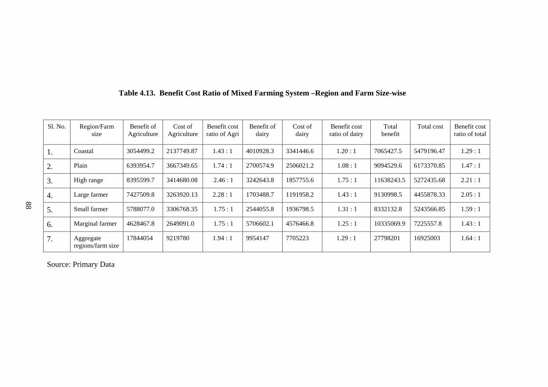
Table 4.13. Benefit Cost Ratio of Mixed Farming System –Region and Farm Size-wise Sl. No.
Region/Farm
size Benefit of
Agriculture Cost of
Agriculture Benefit cost ratio of Agri
Benefit of dairy
Cost of dairy
Benefit cost ratio of dairy
Total benefit
Total cost
Benefit cost ratio of total
1. Coastal 3054499.2 2137749.87 1.43 : 1 4010928.3 3341446.6 1.20 : 1 7065427.5 5479196.47 1.29 : 1
2. Plain 6393954.7 3667349.65 1.74 : 1 2700574.9 2506021.2 1.08 : 1 9094529.6 6173370.85 1.47 : 1
3. High range 8395599.7 3414680.08 2.46 : 1 3242643.8 1857755.6 1.75 : 1 11638243.5 5272435.68 2.21 : 1
4. Large farmer 7427509.8 3263920.13 2.28 : 1 1703488.7 1191958.2 1.43 : 1 9130998.5 4455878.33 2.05 : 1
5. Small farmer 5788077.0 3306768.35 1.75 : 1 2544055.8 1936798.5 1.31 : 1 8332132.8 5243566.85 1.59 : 1
6. Marginal farmer 4628467.8 2649091.0 1.75 : 1 5706602.1 4576466.8 1.25 : 1 10335069.9 7225557.8 1.43 : 1
7. Aggregate regions/farm size
17844054 9219780 1.94 : 1 9954147 7705223 1.29 : 1 27798201 16925003 1.64 : 1
88
Source: Primary Data

The critical value of benefit cost ratio is based on whether the value of the
ratio is greater than one or benefit is greater than cost at a particular point of time.
Though there are many methods to estimate the desirability of an economic
activity or activity mix, benefit cost ratio is simple to calculate and interpret and
also suitable for analyzing an ongoing enterprise.
Table 4.13 shows the benefit cost ratio of crops and dairy separately and
collectively on region and size of farm wise. It could be observed that the benefit
cost ratio was greater than one in all regions and farm sizes for crop, dairy and crop
plus dairy mix enterprises which indicates unambiguously that the activity mix is
desirable and profitable. This finding is in agreement with those of Singh et al.
(1996) whose results indicated that the dairy enterprise in combination with crop
farming had offered considerable scope for increasing the net returns as well as
employment potential of small farms. Papachristoaloulou and Papas (1975) also
found that the combination of livestock and crop enterprise increased costs and
revenues with a net increase in gross and net profit.
Benefit cost ratio was highest for crop cultivation in high range region
followed by plain and coastal region. With regard to the farm size for crop
cultivation, the benefit cost ratio was highest in large farms and that of small and
marginal farm it was even or uniform. It could be observed from Table 4.13 that
benefit cost ratio was highest in large farms since they had more land to cultivate
the crops. In general, benefit cost ratio was lower in dairy activity compared to
crop activity. The lowest benefit cost ratio for dairy activity was among the
marginal farms and in plain region. Looking on benefit cost ratio for mixed
farming in total it could be seen that high range as the region and large farm as the
size group represented the highest benefit cost ratio. They got advantage by
getting better income with cost minimization factors or farm size and ratio were
positively related. It is evident from Table 4.13 as the size of land holding
increased the benefit cost ratio also increased. It implied that higher farm size
might have economies of scale. Benefits also increase as one moves from coastal
to plain and high range.
89

But this finding is in contradiction to that of Elamurugannan (2001) who
found that the cost of cultivation and returns were more or less similar with small
variations among the different types of farms and between groups also.
The major observations of benefit cost ratio analysis can be, thus, summed
up as the following.
(a) Benefit is greater than cost in all regions and farm sizes for both crop
production as well as dairy activity, showing that mixed farming is a desirable
blending.
(b) As the size of farm increased, benefit cost ratio increased, implying economies
of scale in both crop and dairy activities.
(c) Benefit cost ratio improved as one moved from coastal to plain and high range
regions.
(d) Though land was a limiting factor, crop cultivation was relatively beneficial
than dairy. However lion’s share of labour costs accounted for dairy was family
labour which had zero opportunity cost under Kerala conditions and could be
considered as zero cost input, but in the present study market wage rate was
attributed to family labour for cost calculation. Hence wage employment could be
assumed on both sides of cost and benefit of family which would make dairy in a
better competitive edge as an enterprise.
The next section analyses the third objective of the study, that is, input
efficiency and constraints of production in the mixed farming system in Kerala.
4.4 Input Efficiency and Production Constraints
One of the main objectives of a production unit is to coordinate and utilize
resources or factors of production in such a manner that they together yield the
highest net returns. The crux of the problem of growth in agriculture and allied
fields in Kerala is how to increase output per unit of input. One way of
approaching the problem of increasing production is to examine how efficiently the
farmers are using their resources. If resource use is inefficient, production can be
90

increased by making adjustments in the use of factors of production in optimal
direction. In case, it is efficient, the only way out for increasing production would
be the adoption of modern inputs and improved technology of production.
Efficiency is an important concept in the production economics when
resources are meagre and opportunities for developing and adopting better
technologies are competitive. It is also important to know, how well the resources
are being utilized and what possibilities exist for improving operational efficiency.
Efficiency in input resource utilization improves productivity and minimizes the
cost, in effect increases the net return. Efficiency of each input utilized in the
production process is analysed in this section with the help of Cobb-Douglas
production function. Marginal productivity of inputs, returns to scale and
constraints in production/marketing are also examined and analysed, subsequently
based on the results.
4.4.1. Significant Inputs
Production function analysis was used to find out the input-output
relationship, marginal value productivity of inputs used and to examine the
resource use efficiency in crop and milk production in mixed farming. Since gross
income from crop and dairy enterprises was influenced by the land, labour and
capital employed in both crop and dairy enterprises, production function analysis
was carried out to study the input efficiency in mixed farms with respect to the
above mentioned inputs. The production function provides the information in
expected variation in the amount of output like rice, crop productivity and milk
yield when certain quantities of inputs have been changed in proportion.
Since the individual farmer used different types of inputs such as inorganic
fertilizers in crop production, concentrate feeds for the milch animals, alongwith
land and number of milch animals, it is not possible to transform these inputs into
standard comparable inputs. However, the price of each input indirectly reflects
the quality of input. It is, therefore, considered appropriate to express these inputs
in value terms instead of physical terms. Hence for this purpose, a function was
fitted with combined income of the farm from agriculture and dairy in rupees (Y)
91
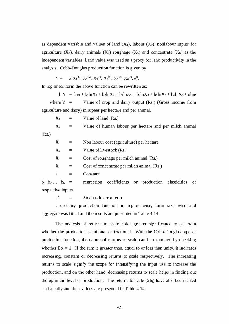
as dependent variable and values of land (X1), labour (X2), nonlabour inputs for
agriculture (X3), dairy animals (X4) roughage (X5) and concentrate (X6) as the
independent variables. Land value was used as a proxy for land productivity in the
analysis. Cobb-Douglas production function is given by
Y = a X1b1. X2
b2. X3b3. X4
b4. X5b5. X6
b6. eu.
In log linear form the above function can be rewritten as:
lnY = lna + b1lnX1 + b2lnX2 + b3lnX3 + b4lnX4 + b5lnX5 + b6lnX6 + ulne
where Y = Value of crop and dairy output (Rs.) (Gross income from
agriculture and dairy) in rupees per hectare and per animal.
X1 = Value of land (Rs.)
X2 = Value of human labour per hectare and per milch animal
(Rs.)
X3 = Non labour cost (agriculture) per hectare
X4 = Value of livestock (Rs.)
X5 = Cost of roughage per milch animal (Rs.)
X6 = Cost of concentrate per milch animal (Rs.)
a = Constant
b1, b2 ….. b6 = regression coefficients or production elasticities of
respective inputs.
eu = Stochastic error term
Crop-dairy production function in region wise, farm size wise and
aggregate was fitted and the results are presented in Table 4.14
The analysis of returns to scale holds greater significance to ascertain
whether the production is rational or irrational. With the Cobb-Douglas type of
production function, the nature of returns to scale can be examined by checking
whether Σbi = 1. If the sum is greater than, equal to or less than unity, it indicates
increasing, constant or decreasing returns to scale respectively. The increasing
returns to scale signify the scope for intensifying the input use to increase the
production, and on the other hand, decreasing returns to scale helps in finding out
the optimum level of production. The returns to scale (Σbi) have also been tested
statistically and their values are presented in Table 4.14.
92
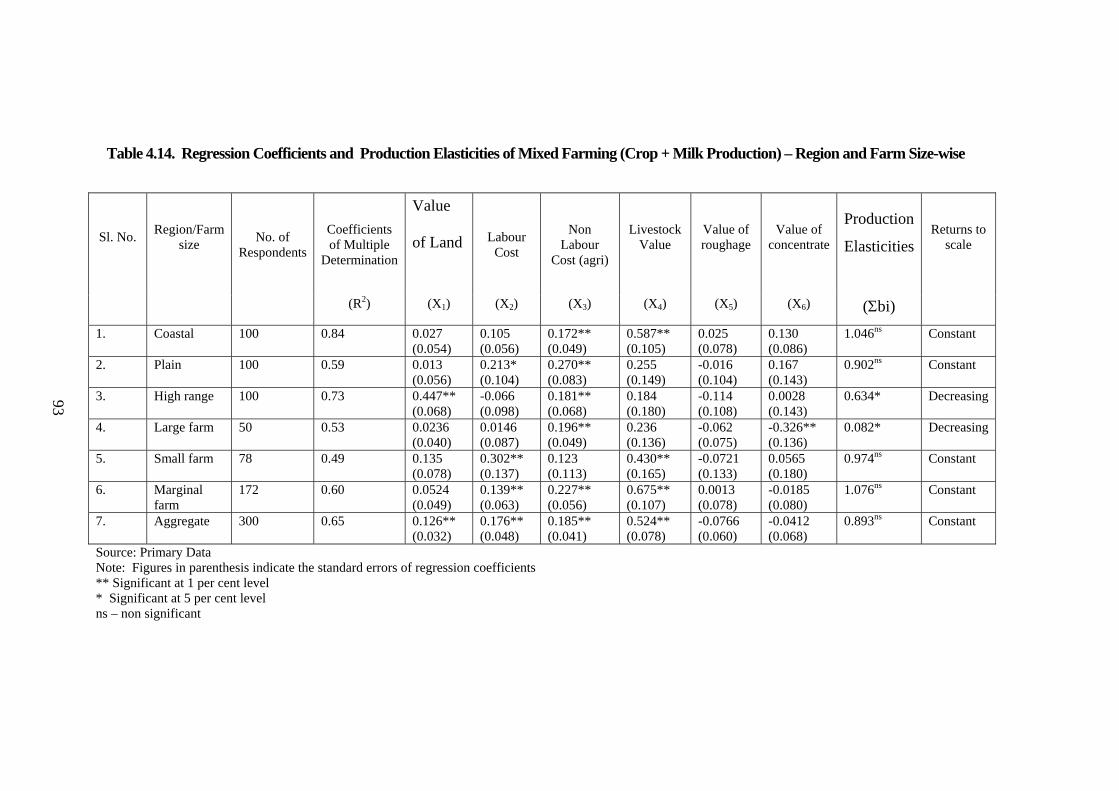
Table 4.14. Regression Coefficients and Production Elasticities of Mixed Farming (Crop + Milk Production) – Region and Farm Size-wise
Sl. No.
Region/Farm size
No. of Respondents
Coefficients of Multiple
Determination
Value
of Land
Labour Cost
Non Labour
Cost (agri)
Livestock Value
Value of roughage
Value of concentrate
Production
Elasticities
Returns to scale
(R2) (X1) (X2) (X3) (X4) (X5) (X6) (Σbi)
1. Coastal 100 0.84 0.027 (0.054)
0.105 (0.056)
0.172** (0.049)
0.587** (0.105)
0.025 (0.078)
0.130 (0.086)
1.046ns Constant
2. Plain 100 0.59 0.013 (0.056)
0.213* (0.104)
0.270** (0.083)
0.255 (0.149)
-0.016 (0.104)
0.167 (0.143)
0.902ns
Constant
3. High range 100 0.73 0.447** (0.068)
-0.066 (0.098)
0.181** (0.068)
0.184 (0.180)
-0.114 (0.108)
0.0028 (0.143)
0.634* Decreasing
4. Large farm 50 0.53 0.0236 (0.040)
0.0146 (0.087)
0.196** (0.049)
0.236 (0.136)
-0.062 (0.075)
-0.326** (0.136)
0.082*
Decreasing
5. Small farm 78 0.49 0.135 (0.078)
0.302** (0.137)
0.123 (0.113)
0.430** (0.165)
-0.0721 (0.133)
0.0565 (0.180)
0.974ns Constant
6. Marginal farm
172 0.60 0.0524 (0.049)
0.139** (0.063)
0.227** (0.056)
0.675** (0.107)
0.0013 (0.078)
-0.0185 (0.080)
1.076ns
Constant
7. Aggregate 300 0.65 0.126** (0.032)
0.176** (0.048)
0.185** (0.041)
0.524** (0.078)
-0.0766 (0.060)
-0.0412 (0.068)
0.893ns Constant
93
Source: Primary Data Note: Figures in parenthesis indicate the standard errors of regression coefficients ** Significant at 1 per cent level * Significant at 5 per cent level ns – non significant

It is observed from the Table 4.14 that regression coefficients with respect
to all regions/all farms indicated that milch animal was the most important factor
responsive to gross income from mixed farming followed by nonlabour cost (agri),
labour cost and land which were highly responsive and statistically significant at
99% level of confidence. This finding is in agreement with that of Elamurugannan
(2001) whose findings revealed that, the four variables namely gross cropped area,
labour used, value of non labour inputs used and the value of animals were found
to have positive coefficient at one per cent level. The regression coefficient for
value of milch animals was 0.524 and significant at one per cent probability level
(99% level confidence), indicating that by increasing the number of milch animals
100 per cent, holding other inputs constant at the geometric mean level the gross
output will increase by 52.4 per cent. The negative coefficient of roughage and
concentrate indicated that there was an excess use of these inputs. This finding has
contradiction with those of Jacob et al. (1971), Rai and Gangwar (1976) and
Ganeshkumar et al. (2000) who reported that the expenditure in concentrate was
found to have positive and significant impact. The farmers of the study area have
to curtail the expenditure on these inputs in order to avoid the loss by inefficient
resource use.
The elasticity coefficient was found to be 0.893 which was not statistically
different from unity indicative of constant returns to scale commonly prevailing
among the selected farmers in Kerala. Sankhayan and Sirohi (1971) also reported
that in the case of seed potato the sum of elasticities was not significantly different
from unity indicating constant returns to sale. The magnitude of individual
elasticity coefficients indicated the relative shares of different factors of production
such as value of land, labour, livestock and nonlabour cost in the total crop and
milk production (output). The coefficient of multiple determination (R2) indicated
that 65 per cent of the variations in the inter-farm output have been explained by
the independent variables taken for analysis.
Taking first of all, coastal region, factors like nonlabour cost (agriculture)
and livestock value contributed positively and significantly towards crop-milk
production. The sum of regression coefficient was worked to be 1.046 which was
94
not statistically different from unity indicative of the constant returns to scale in the
mixed farming operations.
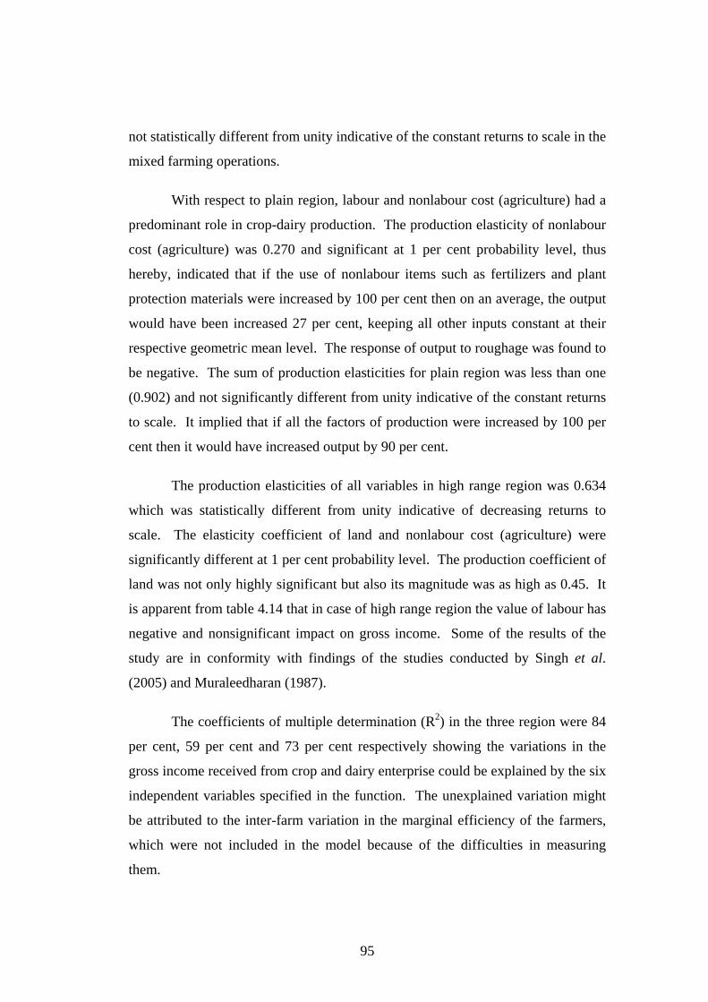
With respect to plain region, labour and nonlabour cost (agriculture) had a
predominant role in crop-dairy production. The production elasticity of nonlabour
cost (agriculture) was 0.270 and significant at 1 per cent probability level, thus
hereby, indicated that if the use of nonlabour items such as fertilizers and plant
protection materials were increased by 100 per cent then on an average, the output
would have been increased 27 per cent, keeping all other inputs constant at their
respective geometric mean level. The response of output to roughage was found to
be negative. The sum of production elasticities for plain region was less than one
(0.902) and not significantly different from unity indicative of the constant returns
to scale. It implied that if all the factors of production were increased by 100 per
cent then it would have increased output by 90 per cent.
The production elasticities of all variables in high range region was 0.634
which was statistically different from unity indicative of decreasing returns to
scale. The elasticity coefficient of land and nonlabour cost (agriculture) were
significantly different at 1 per cent probability level. The production coefficient of
land was not only highly significant but also its magnitude was as high as 0.45. It
is apparent from table 4.14 that in case of high range region the value of labour has
negative and nonsignificant impact on gross income. Some of the results of the
study are in conformity with findings of the studies conducted by Singh et al.
(2005) and Muraleedharan (1987).
The coefficients of multiple determination (R2) in the three region were 84
per cent, 59 per cent and 73 per cent respectively showing the variations in the
gross income received from crop and dairy enterprise could be explained by the six
independent variables specified in the function. The unexplained variation might
be attributed to the inter-farm variation in the marginal efficiency of the farmers,
which were not included in the model because of the difficulties in measuring
them.
95

The production function and the related results for the large, small and
marginal farms are also presented in table 4.14. The regression coefficient for the
large farm was significant and a major part of variations in the inter-farm output
had been explained by the independent variables. The sum of production
elasticities was 0.82 for the large farms, 0.97 for small farms and 1.076 for the
marginal farms. The production elasticity for large farm alone was significantly
different from unity at a probability level of 5 per cent indicative of decreasing
returns to scale. Whereas for small and marginal farms it was not significantly
different from unity and hence constant returns to scale. The elasticity coefficient
of nonlabour cost (agriculture) was significant for large farms and marginal farms
and of labour and livestock value for the small farms and marginal farms. As
contradiction to this finding, Panda (1996) reported that though manure and
fertilizer (nonlabour) turned out to be statistically significant impact influencing
output, all other input coefficients were found to be statistically non significant
indicating that there was a scope for higher use of these resources to increase gross
returns by the farms.
In small and marginal farms it could be observed from the regression
coefficients that milch animals were the most important factors to which output
was highly responsive followed by labour cost. The negative coefficient of
roughage in large farms and small farms indicated that there was an excess use of
this input. In large farms there was an excess use of concentrate feed also. It was
found that the magnitude of elasticity coefficient of livestock value was greater for
the marginal farms than that for the large farms. This implied that the milch
animals had been cared more intensively on the marginal farms as compared to the
small farms. It may be due to the fact that the marginal farmers compensated their
income by increasing the milch animals since they could not expect more income
from their limited land.
96

The major observations available from production function analysis are the
following.
i) The six variables taken together to explain gross income from mixed
farming could explain 65% of the result. Rest of the variations were
from inter-farm differences.
ii) Except concentrates and roughage, all other four variables were
statistically significant in determining the gross income (at one per cent
level).
iii) The negative regression coefficients of roughage and concentrate
showed inefficient use of these variables by farmers beyond the
recommended dosage. It indicates that reduction in their use can
minimize cost without affecting output, so that net returns can be
enhanced.
iv) In general, constant returns to scale prevailed among the respondent
farmers which showed scope of further increase in income.
v) For high range region and large farmers explanatory variables were
more significant in general.
vi) Milch animal was statistically significant for the incomes of coastal
region, small farm, marginal farm and mixed farming in general.
97

4.4.2. Marginal Value of Product (MVP) and Input Efficiency
Marginal value of product of a particular input is calculated by taking the
first order partial derivative of the output (Y) function with respect to
corresponding input (X). In case of Cobb-Douglas production function, since
regression coefficients of inputs give their respective production elasticities, MVP
of all the inputs can be calculated by the formula as given below.
^ Y
Xi
MVP Xi = bi
Where Y = Geometric mean of original value of output.
Xi = Geometric mean of original value of ith input. ^
bi = Regression coefficient or production elasticities of ith input
i = 1, 2, ……….. 6 inputs
A resource or input factor is considered to be used most efficiently if its
marginal value product is first sufficient to meet its cost. Equality of marginal
value product to factor cost is, therefore the basic condition that must be satisfied
to obtain efficient resource use. Input is said to be over utilized if (MVPxi – Pxi) <
Zero, under utilized if (MVPxi – Pxi) > Zero and optimally used if (MVPxi – Pxi) =
Zero. Using “t – test”, the significant difference between MVP and unit price of
input was verified.
Marginal value products of input factors obtained from the estimated
regression equations are shown in Table 4.15 including their statistically
significant difference if any, from marginal factor cost.
98

Table 4.15. Marginal Value Products of Inputs at the Geometric Mean Level – Region and Farm Size-wise
Sl. No.
Region/Farms
Land (X1)
Labour (X2)
Non Labour Cost (Agri) (X3)
Livestock Value (X4)
Value of roughage (X5)
Value of concentrate (X6)
1. Coastal 0.0012** 0.9185 2.0077 1.7527* 0.2744 0.5580
2. Plain 0.0010** 0.8167 1.2486 1.4680 -0.4588 1.2814
3. High range 0.0603** -0.4493* 1.9583 0.9333 -4.2329 0.0352
4. Large farm 0.0182** 0.0775 1.1244 1.648 -2.6015 -4.7837**
5. Small farm 0.0115** 1.2880 0.8164 2.2603 -2.6432 0.5836
6. Marginal farm 0.0028** 1.2382 2.8303** 2.0787** 0.0182 -0.0964**
7. Aggregate 0.0095** 1.0703 1.5464 2.3235** -1.7581* -0.3072**
99
Source: Primary Data Note: i) ** Significantly different from unity at 1 per cent probability level ii) * Significantly different from unity at 5 per cent probability level iii) Factor cost of inputs/resources has been taken as one rupee, since these inputs have been measured in value terms
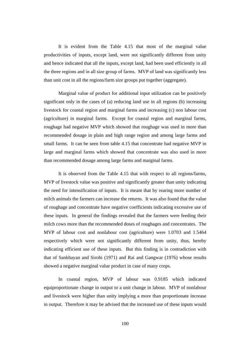
It is evident from the Table 4.15 that most of the marginal value
productivities of inputs, except land, were not significantly different from unity
and hence indicated that all the inputs, except land, had been used efficiently in all
the three regions and in all size group of farms. MVP of land was significantly less
than unit cost in all the regions/farm size groups put together (aggregate).
Marginal value of product for additional input utilization can be positively
significant only in the cases of (a) reducing land use in all regions (b) increasing
livestock for coastal region and marginal farms and increasing (c) non labour cost
(agriculture) in marginal farms. Except for coastal region and marginal farms,
roughage had negative MVP which showed that roughage was used in more than
recommended dosage in plain and high range region and among large farms and
small farms. It can be seen from table 4.15 that concentrate had negative MVP in
large and marginal farms which showed that concentrate was also used in more
than recommended dosage among large farms and marginal farms.
It is observed from the Table 4.15 that with respect to all regions/farms,
MVP of livestock value was positive and significantly greater than unity indicating
the need for intensification of inputs. It is meant that by rearing more number of
milch animals the farmers can increase the returns. It was also found that the value
of roughage and concentrate have negative coefficients indicating excessive use of
these inputs. In general the findings revealed that the farmers were feeding their
milch cows more than the recommended doses of roughages and concentrates. The
MVP of labour cost and nonlabour cost (agriculture) were 1.0703 and 1.5464
respectively which were not significantly different from unity, thus, hereby
indicating efficient use of these inputs. But this finding is in contradiction with
that of Sankhayan and Sirohi (1971) and Rai and Gangwar (1976) whose results
showed a negative marginal value product in case of many crops.
In coastal region, MVP of labour was 0.9185 which indicated
equiproportionate change in output to a unit change in labour. MVP of nonlabour
and livestock were higher than unity implying a more than proportionate increase
in output. Therefore it may be advised that the increased use of these inputs would
100
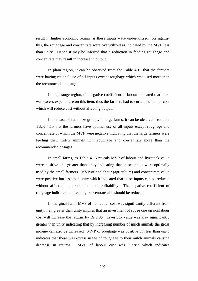
result in higher economic returns as these inputs were underutilized. As against
this, the roughage and concentrate were overutilized as indicated by the MVP less
than unity. Hence it may be inferred that a reduction in feeding roughage and
concentrate may result in increase in output.
In plain region, it can be observed from the Table 4.15 that the farmers
were having rational use of all inputs except roughage which was used more than
the recommended dosage.
In high range region, the negative coefficient of labour indicated that there
was excess expenditure on this item, thus the farmers had to curtail the labour cost
which will reduce cost without affecting output.
In the case of farm size groups, in large farms, it can be observed from the
Table 4.15 that the farmers have optimal use of all inputs except roughage and
concentrate of which the MVP were negative indicating that the large farmers were
feeding their milch animals with roughage and concentrate more than the
recommended dosages.
In small farms, as Table 4.15 reveals MVP of labour and livestock value
were positive and greater than unity indicating that these inputs were optimally
used by the small farmers. MVP of nonlabour (agriculture) and concentrate value
were positive but less than unity which indicated that these inputs can be reduced
without affecting on production and profitability. The negative coefficient of
roughage indicated that feeding concentrate also should be reduced.
In marginal farm, MVP of nonlabour cost was significantly different from
unity, i.e., greater than unity implies that an investment of rupee one on nonlabour
cost will increase the returns by Rs.2.83. Livestock value was also significantly
greater than unity indicating that by increasing number of milch animals the gross
income can also be increased. MVP of roughage was positive but less than unity
indicates that there was excess usage of roughage to their milch animals causing
decrease in returns. MVP of labour cost was 1.2382 which indicates
101

equiproportionate change in output to unit change in labour. It also showed that
the farmers were efficiently using labour input.
The results of resource use efficiency and returns to scale in our analysis
indicate that there exists a vast scope to increase crop and milk production and to
change negative returns into positive by overcoming the inefficient use of different
inputs used particularly feeding roughage and concentrate to the milch animals.
Major results of Table 4.15 can be summed up as following.
(a) There is no scope for increasing income from mixed farming by adding the
component of land to production process with given prices of input and
output in any region or size of farms.
(b) Marginal value of product was negative in the cases of roughages and
concentrates which indicated not only over dose but scope for decreasing
cost without affecting output.
(c) MVP of livestock was greater than one and just the double in aggregate
significantly suggest increasing potential for income from supplying more
milch animals to farmers.
(d) Farmers of high range can reduce the cost by using less labourers without
affecting net returns because marginal productivity of labour is negative.
(e) Marginal farmers have ample scope to increase net returns by incurring
more nonlabour inputs, provided they may get them by loan or grant. One
rupee expense on nonlabour cost can create Rs.2.83 increase in their
output.
(f) Farmers of coastal region and marginal farm size have highest potential to
increase net returns by procuring more milch animals.
102

4.4.3 Production Constraints
This section examines the problems faced by farmers from their own point
of view. Farmers were asked to highlight their problems in both production and
marketing in order of their significance and with the help of Garrett’s ranking
method they are placed in order for the whole group. Methods and results are as
follows.
Since most of the cultivable land in Kerala is dependant on monsoon, the
farmers are often not sure about the outcome from agriculture due to unpredictable
weather. Concentration on crop production alone results in high degree of
uncertainty on farm income and employment. Under the situation of weather and
market induced risk and capital constraints, combining dairy with crop production
by mixed farming helps in stabilizing farm income at a comfortable position.
To reduce the production and market risks, farm diversification and
intensification are considered to be a favourable solution. To increase the farm
income, it is essential to identify the major constraints in production and marketing
of crop and dairy activities and to suggest appropriate constraint management
measures.
Garrett’s ranking method was employed here to assess the relative
significance of problems associated with production and marketing of mixed
farming among the various size groups in the three regions; viz., plain, coastal and
high range region. Garrett’s table is very useful in combining complete order of
merit ratings. The respondents were asked to rank various production and
marketing problems in relation to crop and dairy. The individual’s ranks were
converted into percentage positions for each of the assigned rank by using the
formula
100 (Rij – 0.5) Per cent position = ---------------------- N
103
where,
Rij = Rank assigned for ith category by the jth individual
N = Number of factors ranked by the jth individual
The per cent position of each rank, thus obtained was converted into scores
by referring to the table given by Garrett. For each factor/problem, the scores of
individual respondents were added together and divided by the total number of
respondents for whom the scores were given and thus based on the mean scores,
the ranks were given. These mean scores for all the problems were arranged in
descending order and the most important problem was ranked first and the least
important problem was ranked as the last. The results of Garrett ranking of
production/marketing constraints as expressed by the respondents are furnished in
Table 4.16.
In general it can be observed from Table 4.16 that the most significant
production problems as felt by the farmers for crop husbandry were limited
availability of land, low productivity, crop diseases and labour problems. Some of
the results of the study are in conformity with findings of the study conducted by
Dileep et al. (2002), Agarwal (2003) and Kumar et al. (2004), Mohandas (1994)
identified the nonavailability of labour and increased costs, week infestation and
incidence of pests and diseases as serious constraints as perceived by paddy
farmers. But the finding of the study with regard to crop production is in
contradiction with those Dudhate and Wangikar (2003) who reported that
nonavailability of suitable land for brinjal crop and problems of distant market
were ranked as last problems faced by farmers. Sairam et al. (2003) reported that
incidence of diseases in arecanut was identified as the most important constraint
faced by most of the farmers. Similar findings were reported by Balaji et al. (2003)
in the case of groundnut production.
104

Table 4.16. Garrett’s Ranking of Production/Marketing Constraints of Mixed Farming System – Region and Farm Size-wise
Rank Rank Rank
Sl. No. Constraints Coastal (100)
Plain (100)
High range (100)
Large farmer (50)
Small farmer (78)
Marginal farmer (172)
Overall (300)
I. Crop Production
1.1. Limited land availability II I I -- II I I 1.2 Low productivity VII II III V I II II 1.3 Diseases I III IV IV V III III 1.4 High input cost V VI VII I III IV VI 1.5 Water problem IV V VI III IV V V 1.6 Labour problem III IV V II VII VIII IV 1.7 Transportation cost -- VII VIII VI VI VI VIII 1.8 Wild animals VI -- II VII VIII VII VII
II Crop Marketing
2.1 High brokerage IV II II V IV V III 2.2 Low price III III I I I I I 2.3 High transporting cost II I III II II II II
2.4 Labour problem V VI -- -- V -- VI
2.5 No marketing facilities I IV -- IV III IV IV
2.6 Lack of storage facilities V V -- III VI III V
105

Table 4.16 Contd….
Rank Rank Rank
Sl. No. Constraints Coastal (100)
Plain (100)
High range (100)
Large farmer (50)
Small farmer (78)
Marginal farmer (172)
Overall (300)
III. Milk Production
3.1 Water problem III IV IV IV IV II VI 3.2 High feed cost II I I VII II I I 3.3 Diseases VII II III II III III IV 3.4 Low productivity I -- -- III I IV II
3.5 Lack of knowledge/ information
VI III II I V V III
3.6 Lack of time IV V V VI VI -- V 3.7 Labour cost V -- VI V VII -- VII
IV. Milk Marketing
4.1 No credit availability -- VI -- -- -- -- VI
4.2 Low price II I I III I I I 4.3 Lack of information V III II I III III IV
4.4 Transport distance II V III IV II II II
4.5 No marketing facilities I II IV II IV V III 4.6 Irregular payment from
society IV IV -- V V IV V
106
Source: Primary Data

But in milk production, the most important problems were high feed cost
and low milk yield followed by lack of technical know how and diseases. With
regard to milk production Venkatasubramanian and Fulzele (1996) reported that
high cost of concentrate was one of the constraints perceived by the farmers.
Durggarani and Subhadra (2006) also reported that the most serious problems
related to dairy farming were high cost of concentrate, diseases and low price of
milk as perceived by the farmers.
Important marketing problems for crop were low price, high transportation
cost and high brokerage. Low price and distant location of milk society for selling
milk were also significant marketing constraints for dairy enterprises also. The
constraints in marketing of crops were in agreement with that of Ravisankar and
Katteppa (2000). Kumar et al. (2004) also reported that the problems related to
marketing were low supporting price of produce, and lack of guidance for proper
marketing encounted.
It was found during field survey that majority of the farmers could sell their
produce in their locality itself. Hence, it is noteworthy to mention that the
problems of storage facilities were not important problems faced by the farmers.
The brokerage given to the intermediaries was high and the farmers were getting
low price for their produce. High cost of transportation expressed by many of the
farmers especially in the coastal region might be due to distant location of the
markets and increased hiring charges.
With regard to dairy (milk) marketing, as revealed from table 4.16, low
price for the milk received by the milk producers were the most binding constraint.
Other important problems expressed by the farmers were irregular payment from
milk society and lack of credit availability showing that the farmers could not rely
on milk cooperative societies for selling the milk and getting the credit to get
optimum production from their dairy animals.
107

From the result (Table 4.16) it can be observed that even if the farmers
could buy the inputs with high price for increasing crop production, due to non
availability of land, they were unable to cultivate fodder for their dairy animals.
During the survey, it was found that the farmers were willing to sell their land and
it was slowly picking up as a real estate business. Unfortunately, thus fertile soil is
getting converted from agricultural land into non agricultural land.
Due to limited land availability, dairy farming was constrained to allocate a
proportion of area to grow fodder crop than they were willing to raise any other
cash crop to gain high value products that would enhance their income. The less
important problems perceived by the farmers in milk production were lack of time
and high labour cost. During survey, it could be noticed that the family members
were fully involved in management of dairy animals, hence they were not bothered
about labour cost.
The problems enlisted by the farmers in region wise in the order of
importance are also ranked in Table 4.16. Regarding crop production, the most
binding constraint in the coastal region was diseases, and limited land availability
for both plain region and high range region. Less important problems were low
productivity in coastal region and high transportation cost in both plain and high
range regions. But considering the farm size, large farmers reported that high input
cost as the major problem and destruction of crops by wild animals as the last one.
Low fertility was the most crucial constraint encountered by the small farmers.
This may be due to the fact that the fertile soils were getting converted from
agricultural purposes into nonagricultural purposes. Limited land availability was
found to be the most important problem faced by marginal farmers and hence they
were unable to allocate a proportion of area to grow fodder crop although they
found the most binding constraint in milk production was high feed cost.
Under crop marketing, the most important constraints reported by the
farmers in coastal, plain and high range regions were lack of marketing facilities,
high transportation cost and low price respectively. Labour problem was not
significant among the farmers in coastal and plain regions. It is evident from the
108
Table 4.16 that the most serious problem reported by most of the farmers in
different size group was low price to their produce and least in importance were
lack of storage and marketing facilities.
With regard to milk production, it was the high feed cost which hampered
the dairy farming in the three regions as well as various farm size groups. The
least important problem reported by most of the farmers was labour cost since the
family labour was utilized for dairy farming.
As could be noted from the Table 4.16, that low price of milk was the most
binding constraint in milk marketing at both region wise as well as farm size wise.
Though irregular payment from milk society was also one of the constraints the
farmers were sure that they would get the money after sometime and hence they
were not much bothered about this problem.
Thus, the major constraints in production and marketing of crop cultivation
and dairying as reported by the farmers are as follows (Table 4.16).
(i) Fifteen problems were reported by farmers in the production of crop and
milk together, of which four were common to both activities. Low
productivity was an important problem having second rank in both. But
other generally reported problems such as input cost, timely water
availability and diseases had different rankings. While most crucial problem
to crop production was non availability of land, it was feed cost to milk
production.
(ii) Twelve problems were reported in total by farmers for marketing of
crop and milk, of which three problems were general to both activities. These
general problems had more or less same rank in both crop and milk marketing.
Low price for the product was the most crucial in both cases. Equally important
were transportation problem (cost or distance) and lack of marketing facilities.
109

4.5 Optimum Activity Mix
By looking at input efficiency and production/marketing problems one can
explore methods for optimum conditions in crop/dairy activities of mixed farming
system. In general, many inputs were not in efficient use except livestock at
regional or farm size level. It showed inputs used were not in optimum and
demanded better allocation of resources and use of improved technology. An
optimum activity mix enables the farmer to get more returns from given resources
without any change in technology. It is an ideal condition to maximize income or
minimize cost, so that net returns will be maximum for the farmer with given
resource base. Therefore, this section deals with the possibility of such desirable
change in combination of farming activities which serve the purpose of examining
the fourth objective of study in detail, that is, optimum activity mix of dairy and
crop production to enhance farm income with given technology and resource use
efficiency.
Livestock production as a complementary enterprise to crop production is
an age-old practice which turned to be a more relevant option in an era when no
more land is available for crop cultivation. It is thus necessary to investigate the
size of dairy unit where dairy becomes profitable enterprise in association with
crop cultivation. Linear programming is used as an analytical tool for working out
optimum activity mix at three levels viz., large farmer, small farmer and marginal
farmer, in the three regions viz., coastal, plain and high range in two sections.
4.5.1 Optimum at Regional Level
To find out the optimum activity mix of milch animals with agricultural
crops three types of activity mix were tried viz., agricultural crops with one milch
animal, agricultural crops with two milch animals and agricultural crops with three
milch animals. Sufficient samples were selected to meet this objective. The same
was done separately for different size groups viz. large farm, small farm and
marginal farm and different regions, viz., coastal, plain and highrange.
110

Keeping the area under cultivation fixed, the change was made in the
number of milch animals to find the optimum by using linear programming
technique. For a feasible solution, three optimum conditions were worked out for
each region and farm size. Each condition was different from others with different
input combinations. However an optimum for each condition was worked out by
change of milch animal and keeping the land constant. That is, land area in
existing and optimum condition will be same in same optimization programme but
different for the second and third trials. Number of milch animal alone was
increased one by one in each trial along with a given milch animal or for new
activity mix or optimum I, number of milch animal was two, for optimum II it was
three and for optimum III it was four. Each activity mix was optimized and
represented by optimum one, two and three with no change in land area but milch
animal alone.
The average income of farmers from paddy, homestead and dairy were
maximized subject to the constraints based on available land, labour cost and
nonlabour cost. Average income availability was worked out from optimum
situations for each of the three regions and three farm sizes.
The linear programming model for maximization of the objective function
is given below.
Maximize Z = ΣCjXj
Subject to
ΣjajXj = TA where aj = 1 for j = 2
ΣjbjXj > TL
ΣjdjXj > TNL
Xj > TMin For j = 3 Xj ≤ TMax
Xj ≥ 0
111
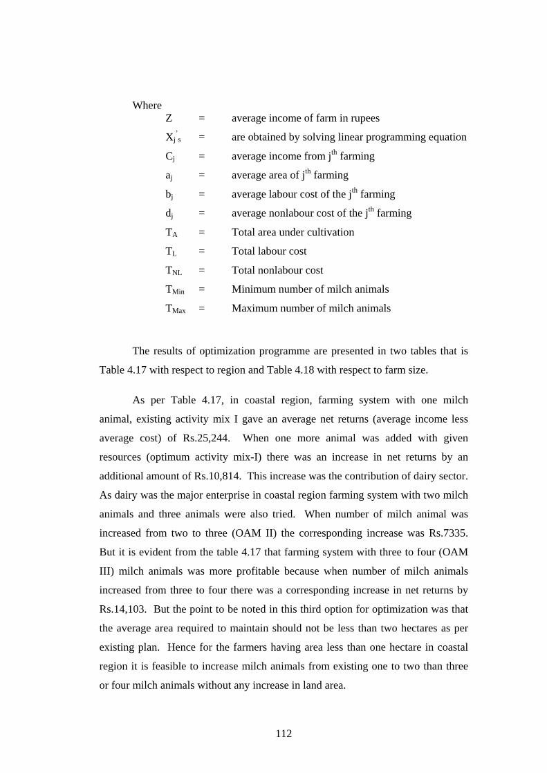
Where Z = average income of farm in rupees
Xj’s = are obtained by solving linear programming equation
Cj = average income from jth farming
aj = average area of jth farming
bj = average labour cost of the jth farming
dj = average nonlabour cost of the jth farming
TA = Total area under cultivation
TL = Total labour cost
TNL = Total nonlabour cost
TMin = Minimum number of milch animals
TMax = Maximum number of milch animals
The results of optimization programme are presented in two tables that is
Table 4.17 with respect to region and Table 4.18 with respect to farm size.
As per Table 4.17, in coastal region, farming system with one milch
animal, existing activity mix I gave an average net returns (average income less
average cost) of Rs.25,244. When one more animal was added with given
resources (optimum activity mix-I) there was an increase in net returns by an
additional amount of Rs.10,814. This increase was the contribution of dairy sector.
As dairy was the major enterprise in coastal region farming system with two milch
animals and three animals were also tried. When number of milch animal was
increased from two to three (OAM II) the corresponding increase was Rs.7335.
But it is evident from the table 4.17 that farming system with three to four (OAM
III) milch animals was more profitable because when number of milch animals
increased from three to four there was a corresponding increase in net returns by
Rs.14,103. But the point to be noted in this third option for optimization was that
the average area required to maintain should not be less than two hectares as per
existing plan. Hence for the farmers having area less than one hectare in coastal
region it is feasible to increase milch animals from existing one to two than three
or four milch animals without any increase in land area.
112

Table 4.17 Optimum Activity Mix of Milch Animals with Agricultural Crops in Mixed Farming – Region wise
Activity Mix (Coastal region) Sl. No.
Activity Unit Existing Optimum
I Existing Optimum
II Existing Optimum
III 1. Total income Rs. 69286 100356 125101 147052 145159 175076 2. Labour Cost Rs. 18470 24367 43905 49055 36640 43547 3. Nonlabour Cost Rs. 25571 39930 37416 46882 43990 52897 4. Net Returns Rs. 25245 36059 43780 51115 64529 78632 5. Incremental
Returns Rs. - 10814 - 7335 - 14103
6. Paddy area Ha 0.42 0.42 0.4 0.4 0.4 0.4 7. Homestead area Ha 0.404 0.404 1.1 1.1 2.16 2.16 8. Milch animals No. 1 2 2 3 3 4
Activity Mix (Plain region) Sl.
No. Activity Unit
Existing Optimum I
Existing Optimum II
Existing Optimum III
1. Total income Rs. 84691 122737 158483 188475 200194 218735 2. Labour Cost Rs. 27676 37174 44728 53625 29222 30542 3. Nonlabour Cost Rs. 21651 35139 26670 3065 68957 78925 4. Net Returns Rs. 35363 50423 91084 104197 102014 109267 5. Incremental
Returns Rs. - 15061 - 13113 - 7253
6. Paddy area Ha 0.5 0.5 0.534 0.534 1.3 1.3 7. Homestead area Ha 0.52 0.52 0.25 0.25 2.15 2.15 8. Milch animals No. 1 2 2 3 3 4
Activity Mix (Highrange region) Sl.
No. Activity Unit
Existing Optimum I
Existing Optimum II
Existing Optimum III
1. Total income Rs. 141233 166334 121001 147342 111306 134936 2. Labour Cost Rs. 31395 35307 23504 25835 12450 13769 3. Nonlabour Cost Rs. 28959 38775 22482 27816 41739 48798 4. Net Returns Rs. 80879 92251 75014 93690 57116 72367 5. Incremental
Returns Rs. - 11372 - 18676 - 15251
6. Paddy area Ha 1.1 1.1 0.58 0.58 0.24 0.24 7. Homestead area Ha 1.26 1.26 1.28 1.28 0.168 0.168 8. Milch animals No. 1 2 2 3 3 4
Source: Computerised result from relevant Primary Data.
113

For plain region the situation was different. Here the farmers did not
depend completely on dairy farming. It is evident from the Table 4.17 that dairy
was not a major enterprise in plain region. As per existing plan farming system
with one milch animal, existing activity mix-I gave an average net return of
Rs.35,363. When one more milch animal was added (optimum activity mix I),
corresponding increase in net return was Rs.15,061. In the case of farming system
with two milch animals if number of milch animal was increased to three it
accounted an increase of net returns by Rs.13,113 and in the third case with four
milch animals the increase in net returns was Rs.7,253. However, as per existing
plan-III even farmers having an average area of not less than two hectares with
three milch animals it is difficult to maintain more than three milch animals per
farm due to high labour cost and nonavailability of land in this region. Hence it
can be concluded that farming systems with one or two more milch animals (OAM
II and OAM III) are more optimum compared to any other plans in plain region.
The average area required was found to be not less than one hectare.
In the case of high range region, an increase in the amount of Rs.11,372
was observed when number of milch animal was increased from one to two. When
optimum solutions were worked out for increasing milch animal from two to three
and three to four it can be seen from the Table 4.17 that corresponding increase in
the amount was Rs.18,676 and Rs.15,251 respectively. Hence it can be suggested
that it is feasible to maintain two to three milch animals than one and four.
Theodore et al. (2001 and 2002) in a more or less similar study reported
that dairy made the difference between diversification (rice + dairy + banana) and
non diversification (rice + banana) in the study area, which influenced significantly
the economy and ecology of the wetland farmers. Papachristodonlou and Papas
(1975) by applying optimization method found that the combination of livestock
and crop enterprise increased costs and revenues with a net increase in gross and
net profit. They also reported that the combination of livestock and crop
enterprises at the rate of about 12 livestock units and 0.133 hectare of operated
land resulted in efficient utilization of available resources.
114

The major findings from Table 4.17 are the following with respect to
optimization of net farm income as objective function with change in milch
animals and no change in land at coastal, plain and high range regions.
i) Highest incremental income (Rs.18,676) for optimum activity mix was
reported in high range for two additional milch animals with less than
two hectare land and lowest (Rs.7,335) in coastal area for less than two
hectare land and two additional milch animals.
ii) Maximum incremental income for coastal (Rs.14,103) region was
possible with an activity mix of three additional milch animals. But for
plain region maximum incremental income (Rs.15,061) was possible
with one more milch animal.
iii) By supplying one milch animal to plain region, two to high range and
three to coastal region, total incremental income could be maximized
among farmers without change of given land area.
4.5.2. Optimum Activity Mix at Farm Size Level
The optimum activity mixes developed for the three farm size groups viz.,
large farm, small farm and marginal farm are given in the table 4.18. The
methodology and objective function remains the same as in the case of regions. It
was assumed that resource use efficiency, resource base and technology were
given with change permissible in number of milch animal alone for finding out
optimum activity mix (OAM) from existing activity mix (EAM) by applying linear
programming method.
115

Table 4.18 Optimum Activity Mix of Milch Animals with Agricultural Crops in Mixed Farming – Farm Size-wise
Activity Mix – Large Farm Sl.
No. Activity Unit
Existing Optimum I
Existing Optimum II
Existing Optimum III
1. Total income Rs. 144500 169501 261057 286279 208093 230560 2. Labour Cost Rs. 36900 42820 46440 51016 39317 43487 3. Nonlabour Cost Rs. 52067 64104 80403 89738 63887 74856 4. Net Returns Rs. 55533 62577 134213 145525 104887 112216 5. Incremental
Returns Rs. - 7044 - 11312 - 7329
6. Paddy area Ha 2.4 2.4 0.5 0.5 0.8 0.8 7. Homestead area Ha 1.6 1.6 2.6 2.6 2.43 2.43 8. Milch animals No. 1 2 2 3 3 4
Activity Mix – Small Farm Sl.
No. Activity Unit
Existing Optimum I
Existing Optimum II
Existing Optimum III
1. Total income Rs. 84910 106914 190224 213074 142855 156371 2. Labour Cost Rs. 28699 34515 42190 46725 40230 42540 3. Nonlabour Cost Rs. 22575 33085 25100 32994 29500 36430 4. Net Returns Rs. 33636 39313 122934 133355 73125 77401 5. Incremental
Returns Rs. - 5677 - 10421 - 4275
6. Paddy area Ha 0.72 0.72 0.5 0.5 0.8 0.8 7. Homestead area Ha 0.57 0.57 1.1 1.1 0.8 0.8 8. Milch animals No. 1 2 2 3 3 4
Activity Mix – Marginal Farm Sl.
No. Activity Unit
Existing Optimum I
Existing Optimum II
Existing Optimum III
1. Total income Rs. 56956 79300 67654 92406 111306 134936 2. Labour Cost Rs. 11715 16905 14130 16998 14640 15960 3. Nonlabour Cost Rs. 17219 29229 17672 25019 41739 48798 4. Net Returns Rs. 28021 33166 35852 50388 54926 70177 5. Incremental
Returns Rs. - 5145 - 14536 - 15252
6. Paddy area Ha 0.4 0.4 0.32 0.32 0.24 0.24 7. Homestead area Ha 0.274 0.274 0.448 0.448 0.168 0.168 8. Milch animals No. 1 2 2 3 3 4
Source: Computerised result from relevant Primary Data.
116

As per Table 4.18 in the existing plan (EAM-I), for farming system with
one milch animal the net return to a large farmer was Rs.55533. When one milch
animal was added to existing stocking of one (OAM-I), keeping the other farming
inputs constant, there was an increase in incremental net returns to Rs.7,044.
Similarly, optimum solutions were worked out by increasing milch animals from
two to three and three to four. From the table 4.18 it could be observed that
corresponding increase in incremental incomes were Rs.11,312 (OAM-II) and
Rs.7,329 (OAM-III) respectively. Hence change from two to three milch animals
(OAM II) was more profitable compared to OAM I and OAM III.
Similar types of changes could be observed in small farms also. The
existing plan (EAM I) gave an average net returns of Rs.33,636. If the number of
milch animals was increased from one to two (OAM-I), their average net returns
rose to Rs.39,313 which accounted an incremental income increase to Rs.5,677. In
the case of farming system with two milch animals (EAM II) when it was
increased to three milch animals (OAM II) it accounted an incremental income
increase of Rs.10,421. When number of milch animals was increased from three to
four (OAM III), there was an incremental income of Rs.4,275 only. Thus it can be
concluded that for the small farmer having land area of one to two hectares,
activity mix with three milch animals (OAM II) was more attractive compared to
the other two plans (OAM-I and OAM-III).
The existing plan in the marginal farm (EAM-I) gave the average income
of Rs.56,956. When the number of milch animal was increased from one to two
(OAM-I) the average net return was Rs.5,145. When optimal solutions were
worked out by increasing milch animals from two to three and three to four there
was increase in the amount to Rs.14,536 (OAM-II) and Rs.15,252 (OAM-III)
respectively. Since there was only small difference in the increase of net returns in
these two plans, these two plans were equally good than the first plan (OAM-I).
The average size of land holding for the marginal farmer was less than one hectare.
It was better to maintain three to four milch animals (OAM-II and OAM-III) than
two milch animals to yield maximum net returns.
117
Similar results of optimum activity was available in the study of Pandey
and Bhogal (1980) who derived the optimal crop and milk production plans for
various farm groups and increase in net returns ranged from 15 to 92 per cent for
different farm sizes by increasing milch animals from two to six.
Thus as per Table 4.18 optimisation of different activity mix with respect to
various farm sizes has shown the following.
(i) The highest amount of incremental income was available from optimum
activity mix III of marginal farmers (Rs.15,252).
(ii) For both large and small farmers, optimum activity mix-II was more
ideal.
(iii) Farm size wise optimization analysis shows that income of different
farm size groups can be enhanced by giving two or more animals to
large, small and marginal farmers with given area of land..
4.5.3 Optimisation Prospects
Our attempt to identify optimum activity mix with the help of linear
programming has highlighted that net income of farmers can be increased by
adopting mixed farming system. It was also shown that under the conditions of
land scarcity in Kerala, optimum activity mix for farmers of different regions and
farm sizes is possible by adding milch animals to their farming system without
changing land input in the existing activity mix. Since farmers were working
under suboptimum conditions, bringing more milch animals to farming activity
will ensure optimum production and enhanced net returns. Milch animals are not
only complementary for an optimization programme but also an insulation against
market and weather risks in agriculture.
For operational efficacy, a cross section analysis of region and farm size are
useful. It can be generally concluded that two to three milch animals are the more
feasible number of addition for an optimum with existing farming practices in all
regions and farm size groups. In the coastal region either two or four milch
118
animals are more attractive with existing farming practices. This is because most
of the farmers are completely depending on dairying. They are producing value
added products and making dairy as a complementary to agriculture. This
observation was very evident as per optimal plan. With regard to plain region, an
addition of one or two milch animals was more feasible because of high labour
cost in this region. Additional two or three milch animals were more feasible in
high range region. This indicated that there should be separate mixed farming
practices for different regions. Marginal farmers of all regions especially of
coastal region may be supplied more milch animals. However in all regions and
sizes an addition to the stock of milch animals varying from one to three heads
resulted in sizeable increase in net returns.
It was observed that wherever dairy constitutes a component of farming
system, even in the optimized farming system, it has appeared as a positive source
of income and employment. Optimization of milch animals with agricultural crops
will not only increase the profit in all the sizes of farm but also will lead to
significant changes in the cropping pattern and increase in the employment of farm
family labour during the most months in a year.
119

4.6 Gender Analysis in Farming Activities
With the transition in technology as well as in composition of labour force,
changes have occurred in the volume and ratio of hired and family labour in
farming activities. Male-female participation ratio in farming has also been
affected by this social and technological transformations. The present section
examines this dimension of gender in farming activities being the fifth objective in
terms of type and volume of work undertaken, role in decision making and pattern
of time use by male and female in farm and family.
In recent years several studies have been conducted about women in
agriculture. Most of these studies were confined to the analysis of activities
performed by women in crop production. Most often, the development planners,
researchers and extensionists make an assumption that women in farming have the
same needs as men. They have often failed to understand that men and women in
farming play different roles, perform different activities, face different constraints
and have different needs.
Gender analysis helps to understand these differences in role and nature of
work. There is also a need for sensitizing people concerned about these facts.
Apart from the role of a homemaker, the women substantially share the agriculture,
dairy and money making activities with the spouse. While most of the dairy related
activities are performed by women, how far they participate in decision making
process related to crop, dairy and economic activities is an important area to be
probed into. Right decision, at the right time, by the right person will not only
avoid unnecessary critical crises but increase effectiveness of decision making.
In order to highlight the gender dimensions of mixed farming present
section has been divided into three parts as follows.
1. Decision making by the respondents alongwith their counterparts in
production and marketing of crop/dairy activities.
120

2. Work participation of the respondents and their counterparts in mixed
farming.
3. Time use pattern of respondent farmers and their counterparts.
4.6.1 Gender Dimensions of Decision Making
The pattern of decision-making varies from region to region and culture to
culture and also based on management practices. Therefore, an attempt has been
made to analyse the decision making pattern of male and female in crop/dairy
production and marketing activities in region and farm size wise.
The data were collected with the help of structured schedule containing
nine crop activities, nine dairy activities and five marketing activities. The
respondents as well as their counterparts were interviewed. It was found that
certain decisions were taken independently while certain decisions were jointly
taken by the family members. Hence decisions were classified according to its
nature as male alone, female alone and jointly by male and female.
Chi-square test was applied to find out whether statistically significant
difference exists between gender in various activities taken for the study and
summary results are presented for production and marketing activities of mixed
farming in Table 4.19 for the sample size as a whole. Detailed results with respect
to three regions and three farm sizes with Chi-square values are available in
Annexure-V.
121
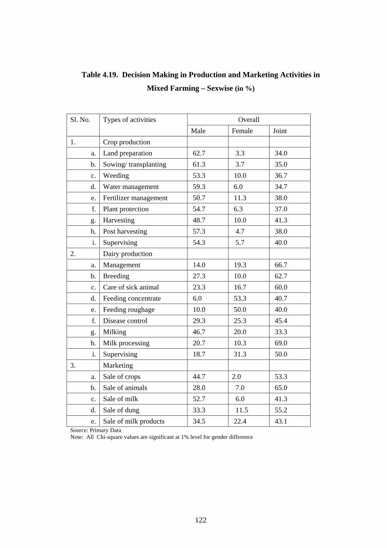
Table 4.19. Decision Making in Production and Marketing Activities in
Mixed Farming – Sexwise (in %)
Overall Sl. No. Types of activities
Male Female Joint 1. Crop production
a. Land preparation 62.7 3.3 34.0 b. Sowing/ transplanting 61.3 3.7 35.0 c. Weeding 53.3 10.0 36.7 d. Water management 59.3 6.0 34.7 e. Fertilizer management 50.7 11.3 38.0 f. Plant protection 54.7 6.3 37.0 g. Harvesting 48.7 10.0 41.3 h. Post harvesting 57.3 4.7 38.0 i. Supervising 54.3 5.7 40.0
2. Dairy production a. Management 14.0 19.3 66.7 b. Breeding 27.3 10.0 62.7 c. Care of sick animal 23.3 16.7 60.0 d. Feeding concentrate 6.0 53.3 40.7 e. Feeding roughage 10.0 50.0 40.0 f. Disease control 29.3 25.3 45.4 g. Milking 46.7 20.0 33.3 h. Milk processing 20.7 10.3 69.0 i. Supervising 18.7 31.3 50.0
3. Marketing a. Sale of crops 44.7 2.0 53.3 b. Sale of animals 28.0 7.0 65.0 c. Sale of milk 52.7 6.0 41.3 d. Sale of dung 33.3 11.5 55.2 e. Sale of milk products 34.5 22.4 43.1
Source: Primary Data Note: All Chi-square values are significant at 1% level for gender difference
122

It could be seen from Table 4.19 that the Chi-square value was higher than
table value in all activities except for sale of milk products in marketing activities.
It is further obvious from the Table 4.19 that for all the crop activities the decisions
were taken predominantly by men. This finding is in agreement with the finding of
Kishore et al. (1999) who reported that regarding pattern of decision making in
preparation of land, sowing, water and fertilizer management and harvesting,
husbands alone took decisions. This finding is in contrast with those of Reddy and
Rashid (1997) who found that most of the decisions relating to agriculture and
horticulture were taken by the farm women. Bhuvaneswari and Kannan (1999),
Kachroo et al. (2003) and Praveena et al. (2005), reported that most of the
decisions in agricultural activities were taken jointly by husband and other family
members. Independent decisions of female were negligible in crop activities. But
in the case of dairy activities, in feeding concentrates and roughages, decisions
were taken mainly by females. This observation is in agreement with those of
Jamal and Arya (2004) who also reported that farm women were involved in the
decision making process in indoor activities like feeding concentrate and fodder.
But this finding is in contradiction to those of Gautam and Tripathi (2001) who
reported that the decision regarding feeding of animals was mostly taken
independently by men. All other decisions were taken jointly by both male and
female. The most important decision of milking was taken by the males. The
decision taken by the males on milking is supported by a similar finding of
Chinnadurai et al. (2002). Majority of other marketing activities were
predominantly a joint decision. This finding is in agreement with the findings of
Kunwar and Kherde (1998), Kishore et al. (1999), Tripathi (1999) and Jamal and
Arya (2004). Male was the major decision maker in 49 per cent cases and female
in seven per cent. However joint decisions were also significant in 44 per cent.
A look at Annexure-V discloses details at regional level. In coastal region
the Chi-square test revealed that the calculated value is higher than table value in
all cases of activities showing that there was significant difference between male
and female in decision making with regard to crop, dairy and marketing activities.
It is interesting to note that in crop activities the decisions were taken either by
123

men or jointly. In the case of dairy activities and marketing except sale of milk
products all the decisions were taken jointly.
In plain region as per Annexure-V, Chi-square test was higher than table
value except for disease control in dairy activities. The perusal of data in Table
4.19 indicates that in crop activities the important decisions were taken by male;
but in dairy activities except for milking most of the decisions were taken jointly.
Females had taken decisions independently in the activities like feeding
concentrate and roughage. In marketing activities the decision were taken by the
males independently.
There was significant difference between male and female in decision
making in high range region also (as per Annexure-V) with regard to all activities
except for land preparation, sowing/transplanting and post harvesting in crop
activities and milking in dairy activities. Women had taken decision on feeding
activities of dairy in this region also. In marketing regarding sale of milk the male
only was taking decisions. In the remaining activities most of the decisions were
taken jointly.
As per Annexure-VI, in the case of large farm the Chi-square test revealed
that the calculated value was higher than table value in the case of all activities
except for harvesting in crop activities and disease control in dairy activities. It is
therefore concluded that there was significant difference between involvement of
male and female in decision making with regard to all activities taken for study.
The perusal of data in table 4.19 indicates that in crop activities most of the
decisions were taken by male, but in dairy activities except for milking most of the
decisions were taken jointly. Females were taking decisions individually in the
feeding activities while the males independently take decisions in milking, sale of
milk and sale of crops and milk.
In small farms (Annexure-VI), it is revealed that the calculated value was
higher than table value in all the cases of activities showing that there was
significant difference between male and female in decision making with regard to
124
crop, dairy and marketing activities. It is also found that in crop activities the
decision was taken either by male or jointly. The females were least involved in
the decision making in crop production. But in dairy activities it could be observed
that except for milking and in all the other activities the decisions were taken
jointly. The males were taking decisions in milking and marketing. In marketing
activities for sale of crop and milk the decisions were taken by men while the
decisions were taken jointly in all the other activities.
There was significant difference between male and female in decision
making in marginal farm with regard to all activities (Annexure-VI). It is obvious
from the Annexure-VI) that for all the crop activities the decisions were taken
predominantly by men. In the case of dairy activities, in feeding practices and
supervision, decisions were taken mainly by females. All other decisions were
taken predominantly by both male and female together in dairy and marketing
activities. Thus it can be concluded that the most of the decisions were taken
jointly in most of the activities in marginal farm.
The major observations of Table 4.19 can be summarised as following.
a) Region and farm size wise analysis of gender dimensions of farm activities in
mixed farming system highlights that male dominated in decision making
process in all occasions of crop production and a few in other activities. While
joint decision was prevailing in 67 per cent cases in dairy production and
marketing activities. The only area where women took independent decision
was in dairy production (33% cases).
b) In general, of the 23 occasions of decision making identified in production and
marketing of crop and dairy activities, males had independent role in 48 per
cent, females had 7 per cent and joint decision of male and female together
were in 45 per cent cases.
c) Though role of women was relatively low in independent decision making
process (07%) joint decision making should be considered as a recognition
given to women in the family set up of farmers.
125

4.6.2 Gender Base of Work Participation
Right and responsibility of decision making and execution are different. It
is due to this difference, role of women in management and work participation in
various farming activities are varying according to the nature of job and custom in
the area. Hence works were basically classified into male or female dominated in
the field. In this section gender base of works are explored and analysed.
Table 4.20 Work Participation in Production and Marketing Activities in
Mixed Farming – Sexwise (in %)
Overall Sl. No. Types of activities
Male Female Joint 1. Crop production
a. Land preparation 80.0 1.7 18.3
b. Sowing/ transplanting 70.7 6.7 22.6
c. Weeding 32.0 39.0 29.0
d. Water management 54.0 14.7 31.3
e. Fertilizer management 22.0 44.7 33.3
f. Plant protection 59.3 11.3 29.4
g. Harvesting 46.7 24.3 29.0
h. Post harvesting 70.0 3.3 26.7
i. Supervising 69.3 5.0 25.7
2. Dairy production
a. Management 19.3 48.0 32.7
b. Breeding 65.3 12.0 22.7
c. Care of sick animal 50.0 26.0 24.0
d. Feeding concentrate 10.7 68.3 21.0
e. Feeding roughage 13.3 64.3 22.4
f. Disease control 36.7 36.7 26.6
g. Milking 56.0 16.7 27.3
h. Milk processing 43.6 44.4 12.0
i. Supervising 20.0 43.3 36.7
3. Marketing
a. Sale of crops 66.7 6.0 27.3
b. Sale of animals 41.3 16.7 42.0
c. Sale of milk 72.0 5.7 22.3
d. Sale of dung 16.7 13.3 70.0
e. Sale of milk products 16.7 61.1 22.2 Source: Primary Data Note: All Chi-square values are significant at 1% level
126

Chi-square test was employed to find out the difference between gender
and participation of members in various farming activities (See Annexure VII &
VIII for details of Chi-square values for region and farmsize wise respectively).
About 23 activities are listed in crop/dairy production and marketing and results
are presented in Table 4.20.
As per Table 4.20, there was significant difference between male and
female in performing all the activities except weeding in crops activities both at
region wise and farm size wise. It is further obvious from the Table 4.20 that land
preparation, sowing/transplanting, water management, plant protection, harvesting,
post harvesting, supervising and marketing were male dominated, while weeding
and fertilizer management were female dominated activities in crop production.
This observation is supported by a similar finding of Usharani et al. (1993) and
Joshi (2000). But in dairy production most of the activities except caring of
animals for both breeding and treatment and milking were performed by women.
Christy and Thirunavukkarasu (2002) and Kanwar and Rekha (2006) also reported
that most of the tasks related to livestock keeping were performed by farm women.
But according to Sureshkumar et al. (1998) majority of farmers jointly participated
in most of the animal husbandry activities. In marketing activities the sale of crops,
sale of milk and certain other activities were alone by male while three other
activities were undertaken jointly. It is clear from the findings that most of the
indoor activities were performed by women.
It can be seen from Annexure-VII that in coastal region harvesting was
performed jointly while all the other eight activities in crop were performed by
men. In the case of dairy production, except milk processing other activities were
done by men and women together. In marketing activities, sale of crop and milk
were performed by men. All the other activities were performed by men and
women together.
In plain region (see Annexure-VII), the Chi-square test revealed that the
calculated value was higher than table value in all cases except for sale of animals
in marketing activities. So the finding reveals that there was no significant
127

difference between male and female in performing the marketing activities like
sale of animals in the plain region. The finding also reveals that in crop production
except weeding and fertilizer management the involvement of men was more in
other activities. Weeding and fertilizer management were performed by women.
But it can be seen that in the case of dairy production, the activities like breeding,
care of sick animals, milking and marketing were performed by male farmers while
in the activities like management, feeding, disease control and supervising, the
female participation was found to be more. In marketing activities, the sale of
crops and milk were performed by men.
The Chi-square test reveals that there was significant difference between
men and women in performing all the crop, dairy and marketing activities in high
range region (Annexure-VII). The findings in Annexure-VI reveals that the
activities like land preparation, sowing/transplanting, water management, plant
protection, post harvesting and supervising were performed by men while the
participation of women was more in weeding, fertilizer management and
harvesting activities in crop production. But it was seen that in the case of dairy
production the activities like breeding, care of sick animals, disease control,
milking and marketing were performed by men, while in the activities like
management, feeding, milk processing and supervising the female participation
was found to be more. In marketing activities the sale of crops and milk were
performed by men.
Annexure-VIII also reveals the work participation/sharing between men
and women in farm group wise. Fifty large farmers, 78 small farmers and 172
marginal farmers in the three regions constituted the sample size.
As per Annexure-VIII the Chi-square test reveals that there was significant
difference between male and female in performing the crop activities except
weeding and harvesting, in dairy activities except feeding practices and supervision
and in marketing activities sale of animals in large farms. It is also evident that
supervision of crop activities, care and breeding of milch animals, milking, sale of
crop, dairy and byproducts were performed by men.
128

In small farms (Annexure-VIII) the Chi-square test reveals that there was
significant difference between male and female in performing all the activities.
Except harvesting activity all the eight activities were performed by male and
harvesting activity was done jointly. But in dairy production activities like
management, feeding, disease control and milk processing were performed by
women showing that most of the indoor activities was done by women. It is an
interesting fact that in marketing activities except sale of animals other activities
were predominantly done by men.
In marginal farms also (Annexure-VIII) the chi-square test reveals that
there was significant difference between male and female in performing all the
crop, dairy and marketing activities. In crop production only weeding and
fertilizer management were performed by women while other activities were
performed predominantly by men. In dairy production taking care of animals for
breeding and treatment, milking and marketing were performed by men while all
the other activities were done predominantly by women. The results of the study
conducted by Varma and Sinha (1992) clearly revealed that animal husbandry was
predominantly a male affair in case of farmers of high socio-economic status
whereas it was predominantly a female affair in case of the farmers of medium and
low socio-economic status. The sale of crops was performed mostly by men.
Though farm activities were generally assumed to be female oriented, as
per Table 4.20 the lion’s share of farm activities under study (59.3%) were
undertaken by male. This was due to their larger share in crop husbandry (78%).
Dairy production was dominated by (56%) female and marketing activities by male
(56%). Farming as a family oriented activity was contributed by male and female
members. Though the work participation was mainly male oriented (59%),
management decision was not that much male oriented (48%). Also joint activity
was more important in management decision (45%) than in work sharing (11%).
Independent involvement for women was higher in farm work participation
(29.6%) than in management decision (7%).
129
4.6.4 Gender and Time Use Pattern
Gender’s role in agricultural production and household activities with
respect to time use pattern of 24 hours are the contents of this section.
The study focused on describing how men and women utilize their given
time and reflect their roles in agricultural and household activities. Data were
collected through field observations, discussion and interviewing the respondents
along with their counterparts by using structured interview schedule. Findings are
presented in Table 4.21 which shows the detailed time use pattern of the husbands
and wives for their daily activities in 24 hours in the three regions as well as three
farm size groups together.
Table 4.21 shows a comparison of the time use of men and women in the
family for doing various daily activities inside and outside the family households.
It could be observed from the Table 4.21 that among the production activities, men
spent more time in crop activities while women spent more time in dairy activities.
Women spent their lion’s share of time in household activities while men were
more involved in recreation, nonagricultural activities. This finding is in
agreement with that of Kunwar et al. (1997) who reported that rural women of
district Rampur participated in home activities more than farm activities. But this
finding is in contradiction to those of Singh and Garia (1999) who found that the
total working hours spent by adult females accounted for 85 per cent of agricultural
work, 81 per cent of work related to animal husbandry and 84 per cent of domestic
work. According to Sheela and Katteppa (1999) marginal farm women spent
maximum time in farm activities, small farm women on household activities and
large farm women on resting and other leisure time activities. It could also be
observed that men spent more time for recreation, non agricultural activities and
sleeping than women. Women had spent more time than men only in dairy
production and household works.
130
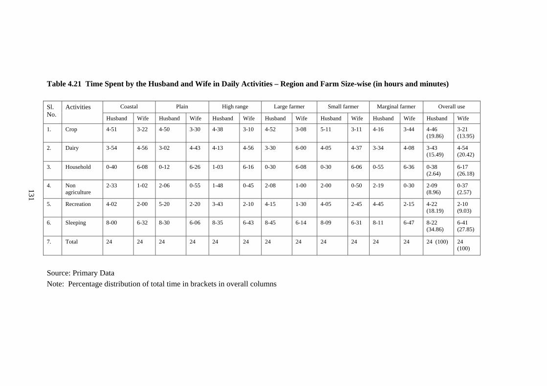
Table 4.21 Time Spent by the Husband and Wife in Daily Activities – Region and Farm Size-wise (in hours and minutes)
Coastal Plain High range Large farmer Small farmer Marginal farmer Overall use Sl. No.
Activities
Husband Wife Husband Wife Husband Wife Husband Wife Husband Wife Husband Wife Husband Wife
1. Crop 4-51 3-22 4-50 3-30 4-38 3-10 4-52 3-08 5-11 3-11 4-16 3-44 4-46 (19.86)
3-21 (13.95)
2. Dairy 3-54 4-56 3-02 4-43 4-13 4-56 3-30 6-00 4-05 4-37 3-34 4-08 3-43 (15.49)
4-54 (20.42)
3. Household 0-40 6-08 0-12 6-26 1-03 6-16 0-30 6-08 0-30 6-06 0-55 6-36 0-38 (2.64)
6-17 (26.18)
4. Non agriculture
2-33 1-02 2-06 0-55 1-48 0-45 2-08 1-00 2-00 0-50 2-19 0-30 2-09 (8.96)
0-37 (2.57)
5. Recreation 4-02 2-00 5-20 2-20 3-43 2-10 4-15 1-30 4-05 2-45 4-45 2-15 4-22 (18.19)
2-10 (9.03)
6. Sleeping 8-00 6-32 8-30 6-06 8-35 6-43 8-45 6-14 8-09 6-31 8-11 6-47 8-22 (34.86)
6-41 (27.85)
7. Total 24 24 24 24 24 24 24 24 24 24 24 24 24 (100) 24 (100)
131
Source: Primary Data Note: Percentage distribution of total time in brackets in overall columns

Thus it can be concluded that most of the crop activities were attended to
by men while dairy activities were done by women. On an average both men and
women spent eight hours for directly productive activities. According to Joshi
(2000) the time use profile showed that women worked 12 or 13 hours a day while
men worked only eight or nine hours a day depending on the season. But women’s
work continued in households. While men took 53% of their time for recreation
and sleep, women took only 37% of their time for the same purpose.
General observations by analysing the data with respect to gender in time
use pattern are as follows:
i) Male dominance was prevailing in general in mixed farming system
which combines crop husbandry and livestock production.
ii) Predominance of male in work participation in crop production is
pronounced.
iii) Decision making was an area where male and female members were
mutually participating.
iv) Female work was more confined to domestication of milch animals and
indoor work for the family.
v) Females were entrusted with major share of unpaid work whether it was
rearing of milch animals or cooking of food at home.
Analysis of gender dimensions of farm activities and time use pattern
reiterated the existing social structure where male dominance prevailed. But things
are changing as seen in the analysis that decision making at home turn to be more
and more participative.
132

4.7 Conclusions
The study on Economics of mixed farming system was intended to examine
five objectives in detail such as (a) existing mixed farming practices, (b) benefit
cost analysis, (c) input efficiency, (d) optimum activity mix and (e) gender
dimensions. Mixed farming as a natural outcome of economic compulsions of
maximizing farm income from given resources of farmers by a harmonious
combination of crop and livestock production varied widely in resource base and
resource use efficiency in different regions and sizes of farms. Benefit per unit of
cost was always greater than unity. Input efficiency, though varied with respect to
inputs, regions and farm sizes, in general highlighted excess use of cattle feeds.
With a realistic assumption of no change in area of land and given resource use
efficiency, it was found that addition of milch animals could increase net returns of
farmers considerably. The results with regard to the final objective of gender
dimensions went in conformity with the general male dominance in paid work but
indicated increased role of joint decision in family by both male and female.
The results of the study have significant policy implications. They suggest
not only region wise and class wise measures to improve farm income but exhibits
sound complementarity between crop and livestock production. As such the
commencing final chapter examines the implications of inferences drawn from the
analysis and a few suggestions to improve the farm income based on these
inferences and implications.
133