chapter 4: measuring execution time - college of...

Chapter 4: Measuring Execution Time 1

Chapter 4: Measuring Execution Time

You would think that measuring the execution time of a program would be easy. Simply

use a stopwatch, start the program, and notice how much time it takes until the program

ends. But this sort of measurement, called a wall-clock time,

is for several reasons not the best characterization of a

computer algorithm. A benchmark describes only the

performance of a program on a specific machine on a given

day. Different processors can have dramatically different

performances. Even working on the same machine, there

may be a selection of many alternative compilers for the

same programming language. For this and other reasons,

computer scientists prefer to measure execution time in a

more abstract fashion.

Algorithmic Analysis

Why do dictionaries list words in alphabetical order? The answer may seem obvious, but

it nevertheless can lead to a better understanding of how to abstractly measure execution

time. Perform the following mind experiment.

Suppose somebody were to ask you to look up the

telephone number for “Chris Smith” in the directory

for a large city. How long would it take? Now,

suppose they asked you to find the name of the

person with number 564-8734. Would you do it? How long do you think it would take?

Is there a way to quantify this intuitive feeling that searching an ordered list is faster than

searching an unordered one? Suppose n represents the number of words in a collection. In

an unordered list you must compare the target word to each list word in turn. This is

called a linear search. If the search is futile; that is, the word is not on the list, you will

end up performing n comparisons. Assume that the amount of time it takes to do a

comparison is a constant. You don’t need to know what the constant is; in fact it really

doesn’t matter what the constant is. What is important is that the total amount of work

you will perform is proportional to n. That is to say, if you were to search a list of 2000

words it would take twice as long as it would to search a list of 1000 words. Now

suppose the search is successful; that is, the word is found on the list. We have no idea

where it might be found, so on average we would expect to search half the list. So the

expectation is still that you will have to perform about n/2 comparisons. Again, this value

is proportional to the length of the list – if you double the length of the list, you would

expect to do twice as much work.

What about searching an ordered list? Searching a dictionary or a phonebook can be

informally described as follows: you divide the list in half after each comparison. That is,

after you compare to the middle word you toss away either the first half or the last half of

the list, and continue searching the remaining, and so on each step. In an earlier chapter

Abby Smith 954-9845 Chris Smith 234-7832 Fred Smith 435-3545 Jaimie Smith 845-2395 Robin Smith 436-9834


you learned that this is termed a binary search. If you have been doing the worksheets

you have seen binary search already in worksheet 5. Binary search is similar to the way

you guess a number if somebody says “I’m thinking of a value between 0 and 100. Can

you find my number?” To determine the speed of this algorithm, we have to ask how

many times can you divide a collection of n elements in half.

To find out, you need to remember some basic facts about two functions, the exponential

and the logarithm. The exponential is the function you get by repeated multiplication. In

computer science we almost always use powers of two, and so the exponential sequence

is 1, 2, 4, 8, 16, 32, 64, 128, 256, 512, 1024, and so on. The logarithm is the inverse of

the exponential. It is the number that a base (generally 2) must be raised to in order to

find a value. If we want the log (base 2) of 1000, for example, we know that it must be

between 9 and 10. This is because 29 is 512, and 2

10 is 1024. Since 1000 is between these

two values, the log of 1000 must be between 9 and 10. The log is a very slow growing

function. The log of one million is less than 20, and the log of one billion is less than 30.

It is the log that provides the

answer to our question. Suppose

you start with 1000 words. After

one comparison you have 500,

after the second you have 250,

after the third 125, then 63, then

32, then 16, 8, 4, 2 and finally 1.

Compare this to the earlier

exponential sequence. The values

are listed in reverse order, but can

never be larger than the

corresponding value in the

exponential series. The log

function is an approximation to

the number of times that a group

can be divided. We say

approximation because the log

function returns a fractional value, and we want an integer. But the integer we seek is

never larger than 1 plus the ceiling (that is, next larger integer) of the log.

Performing a binary search of an ordered list containing n words you will examine

approximately log n words. You don’t need to know the exact amount of time it takes to

perform a single comparison, as it doesn’t really matter. Represent this by some unknown

quantity c, so that the time it takes to search a list of n words is represented by c * log n.

This analysis tells us is the amount of time you expect to spend searching if, for example,

you double the size of the list. If you next search an ordered collection of 2n words, you

would expect the search to require c * log (2n) steps. But this is c * (log 2 + log n). The

log 2 is just 1, and so this is nothing more than c + c * log n or c * (1 + log n).

Intuitively, what this is saying is that if you double the size of the list, you will expect to

perform just one more comparison. This is considerably better than in the unordered list,

Logarithms

To the mathematician, a logarithm is envisioned

as the inverse of the exponential function, or as a

solution to an integral equation. However, to a

computer scientist, the log is something very

different. The log, base 2, of a value n is

approximately equal to the number of times that

n can be split in half. The word approximately is

used because the log function yields a fractional

value, and the exact figure can be as much as

one larger than the integer ceiling of the log. But

integer differences are normally ignored when

discussing asymptotic bounds. Logs occur in a

great many situations as the result of dividing a

value repeatedly in half.


where if you doubled the size of the list you doubled the number of comparisons that you

would expect to perform.

Big Oh notation

There is a standard notation that is used to simplify the comparison between two or more

algorithms. We say that a linear search is a O(n) algorithm (read “big-Oh of n”), while a

binary search is a O(log n) algorithm (“big-Oh of log n”).

The idea captured by big-Oh notation is like the concept of the derivative in calculus. It

represents the rate of growth of the execution time as the number of elements increases,

or -time versus -size. Saying that an algorithm is O(n) means that the execution time is

bounded by some constant times n. Write this as c*n. If the size of the collection doubles,

then the execution time is c*(2n). But this is 2*(c*n), and so you expect that the

execution time will double as well. On the other hand, if a search algorithm is O(log n)

and you double the size of the collection, you go from c*(log n) to c*(log 2n), which is

simply c + c*log n. This means that O(log n) algorithms are much faster than O(n)

algorithms, and this difference only increases as the value of n increases.

A task that requires the same amount of time regardless of the input size is described as

O(1), or “constant time”. A task that is O(n) is termed a linear time task. One that is

O(log n) is called logarithmic. Other terms that are used include quadratic for O(n2)

tasks, and cubic for O(n3) algorithms.

What a big-oh characterization of an algorithm does is to abstract away unimportant

distinctions caused by factors such as different machines or different compilers. Instead,

it goes to the heart of the key differences between algorithms. The discovery of a big-oh

characterization of an algorithm is an important aspect of algorithmic analysis. Due to the

connection to calculus and the fact that the big-oh characterization becomes more

relevant as n grows larger this is also often termed asymptotic analysis. We will use the

two terms interchangeably throughout this text.

In worksheet 8 you will investigate the big-Oh characterization of several simple

algorithms.

Summing Execution Times

If you have ever sat in a car on a rainy day you might have noticed

that small drops of rain can remain in place on the windscreen, but

as a drop gets larger it will eventually fall. To see why, think of the

forces acting on the drop. The force holding the drop in place is

surface tension. The force making it fall is gravity. If we imagine

the drop as a perfect sphere, the surface tension is proportional to the square of the radius,

while the force of gravity is proportional to the volume, which grows as the cube of the

radius. What you observe is that no matter what constants are placed in front of these two


values, a cubic function (c * r3 , i.e. gravity) will eventually grow larger than a quadratic

function (d * r2 , i.e. surface tension).

The same idea is used in algorithmic analysis. We say that one function dominates

another if as the input gets larger the second will

always be larger than the first, regardless of any

constants involved. To see how this relates to

algorithms consider the function to initialize an

identity matrix. If you apply the techniques from

the worksheets it is clear the first part is

performing O(n2) work, while the second is O(n).

So you might think that the algorithm is O(n2+n).

But instead, the rule is that when summing big-

Oh values you throw away everything except the

dominating function. Since n2 dominates n, the algorithm is said to be O(n

2).

What functions dominate each

other? The table below lists

functions in order from most

costly to least. The middle

column is the common name for

the function. The third column

can be used to illustrate why the

dominating rule makes sense.

Assume that an input is size 105,

and you can perform 106

operations per second. The third

column shows the approximate

time it would take to perform a

task if the algorithm is of the

given complexity. So imagine that we had an algorithm had one part that was O(n2) and

another that was O(n). The O(n2) part would be taking about 2.8 hours, while the O(n)

part would contribute about 0.1 seconds.

The smaller value gets overwhelmed by

the larger.

In worksheet 9 you will explore several

variations on the idea of dominating

functions.

Each of the functions commonly found as

execution times has a characteristic shape

when plotted as a graph. Some of these

are shown at right. With experience you

should be able to look at a plot and

recognize the type of curve it represents.

Function Common name Running time N! Factorial 2

n Exponential > century N

d, d > 3 Polynomial

N3 Cubic 31.7 years

N2 Quadratic 2.8 hours

N sqrt n 31.6 seconds N log n 1.2 seconds N Linear 0.1 second sqrt (n) Root-n 3.2 * 10

-4 seconds

Log n Logarithmic 1.2 * 10-5

seconds 1 Constant

void makeIdentity (int m[N][N]) {

for (int i = 0; i < N; i++)

for (int j = 0; j < N; j++)

m[i][j] = 0;

for (int i = 0; i < N; i++)

m[i][i] = 1;

}

10

8

6

4

2

0

0

2

4

6

8

10

linear quadratic

cubic root-n log n

constant


The Limits of big-Oh

The formal definition of big-Oh states that if f(n) is a function that represents the actual

execution time of an algorithm, the algorithm is O(g(n)) if, for all values n larger than a

fixed constant n0, there exists a constant c, such that f(n) is always bounded by (that is,

smaller than or equal to) the quantity c * g(n). Although this formal definition may be of

critical importance to theoreticians, an intuitive felling for algorithm execution is of more

practical importance.

The big-oh characterization of algorithms is designed to measure the behavior as inputs

become ever larger. They may not be useful when n is small. In fact, for small values of n

it may be that an O(n2) algorithm, for example, is faster than an O(n log n) algorithm,

because the constants involve mask the asymptotic behavior. A real life example of this is

matrix multiplication. There are algorithms for matrix multiplication that are known to be

faster than the naïve O(n3) algorithm shown in worksheet 8. However, these algorithms

are much more complicated, and since the value n (representing the number of rows or

columns in a matrix) seldom gets very large, the classic algorithm is in practice faster.

Another limitation of a big-oh characterization is that it does not consider memory usage.

There are algorithms that are theoretically fast, but use an excessively large amount of

memory. In situations such as this a slower algorithm that uses less memory may be

preferable in practice.

Using Big-Oh to Estimate Wall Clock Time

A big-Oh description of an algorithm is a characterization of the change in execution

time as the input size changes. If you have actual execution timings (“wall clock time”)

for an algorithm with one input size, you can use the big-Oh to estimate the execution

time for a different input size. The fundamental equation says that the ratio of the big-

Oh’s is equal to the ratio of the execution times. If an algorithm is O(f(n)), and you know

that on input n1 it takes time t1, and you want to find the time t2 it will take to process an

input of size n2, you create the equation

f(n1) / f(n2) = t1 / t2

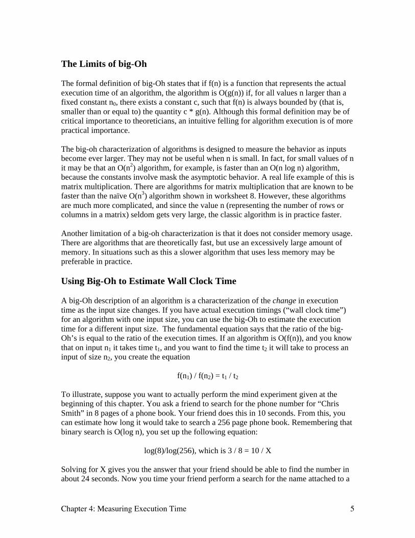
To illustrate, suppose you want to actually perform the mind experiment given at the

beginning of this chapter. You ask a friend to search for the phone number for “Chris

Smith” in 8 pages of a phone book. Your friend does this in 10 seconds. From this, you

can estimate how long it would take to search a 256 page phone book. Remembering that

binary search is O(log n), you set up the following equation:

log(8)/log(256), which is 3 / 8 = 10 / X

Solving for X gives you the answer that your friend should be able to find the number in

about 24 seconds. Now you time your friend perform a search for the name attached to a


given number in the same 8 pages. This time your friend takes 2 minutes. Recalling that a

linear search is O(n), this tells you that to search a 256 page phone could would require:

8/256 = 2 / X

Solving for X tells you that your friend would need about 64 minutes, or about an hour.

So a binary search is really faster than a linear search.

In Worksheet 10 you will use this equation to estimate various different execution times.

Recursive Functions and Recurrence Relations The analysis of recursive functions is slightly more complicated than the analysis of

algorithms with loops. A useful technique is to describe the execution time using a

recurrence relation. To illustrate, consider a function to print a positive integer value in

binary format. Here n will represent the number of binary digits in the printed form.

Because the argument is divided by 2 prior to the recursive call, it will have one fewer

digit. Everything else, outside of the recursive call,

can be performed in constant time. The base case can

also be performed in constant time. If we let T(n)

represent the time necessary to print an n-digit

number, we have the following equation:

T(n) = T(n-1) + c

T(1) = c

Read this as asserting that the time for n is equal to

the time for n-1 plus some unknown constant value. Whenever you see this relation you

can say that the running time of the recursive function is O(n). To see why, remember

that O(n) means that the actual running time is some constant times n plus other constant

values. Let us write this as c1n + c2. To verify that this is the solution to the equation,

substitute for both sides, and show that the results are equal if the constants are in the

correct relation. T(n) is c1n + c2. We want this to be equal to c1(n-1) + c2 + c. But the

latter is c1n + c2 + c – c1. Hence the two sides are equal if c is equal to c1. In general we

can just merge all constants into one constant value.

The four most common recurrence

relations and their solutions are shown at

left. Here we simply assert these solutions

without proof. However, it is not difficult

to check that the solutions are reasonable.

For example, to verify the second you can observe the following

c1 * log n + c = c1 * (log (n/2)) + c = c1 * (log n – 1) + c = c1 * log n + c

T(n) = T(n-1) + c O(n) T(n) = T(n/2) + c O(log n) T(n) = 2 * T(n/2) + ca n + cb O(n log n) T(n) = 2 * T(n-1) + c O(2

n)

void printBinary (int v) { if ((v == 0) || (v == 1)) print(n); else { printBinary(v/2); print(v%2); } }


In worksheet 11 you will use these forms to estimate the running time of various

recursive algorithms. An analysis exercise at the end of this chapter asks you to verify

the solution of each of these equations.

Best and Worst Case Execution Time

The bubble sort and selection sort algorithms require the same amount of time to execute,

regardless of the input. However, for many algorithms the execution time will depend

upon the input values, often dramatically so. In these situations it is useful to understand

the best situation, termed the best case time, and the worst possibility, termed the worst

case time. We can illustrate this type of analysis with yet another sorting algorithm. This

algorithm is termed insertion sort. If you have been doing the worksheets you will

remember this from worksheet 7.

The insertion sort algorithm is most easily described by considering a point in the middle

of execution:

2 3 4 7 9 5 1 8 6 0

P already sorted Yet to be considered

Let p represent an index position in the middle of an array. At this point the elements to

the left of p (those with index values smaller than p) have already been sorted. Those to

the right of p are completely unknown. The immediate task is simply to place the one

element that is found at location p so that it, too, will be part of the sorted portion. To do

this, the value at location p is compared to its neighbor. If it is smaller, it is swapped with

its neighbor. It is then compared with the next element, possibly swapped, and so on.

2 3 4 7 5 9 1 8 6 0

This process continues until one of two conditions occur. Either a value is found that is

smaller, and so the ordering is established, or the value is swapped clear to the start of the

array.

2 3 4 5 7 9 1 8 6 0

1 2 3 4 5 7 9 8 6 0


Since we are using a while loop the analysis of execution time is not as easy as it was for

selection sort.

Question: What type of value will make your loop execute the fewest number of

iterations? What type of value will make your loop execute the largest number of times?

If there are n elements to the left of p, how many times will the loop iterate in the worst

case? Based on your observations, can you say what type of input will make the insertion

sort algorithm run most quickly? Can you characterize the running time as big-Oh?

What type of input will make the insertion sort algorithm run most slowly? Can you

characterize the running time as big-Oh?

We describe this difference in execution times by saying that one value represents the

best case execution time, while the other represents the worst case time. In practice we

are also interested in a third possibility, the average case time. But averages can be tricky

– not only can the mathematics be complex, but the meaning is also unclear. Does

average mean a random collection of input values? Or does it mean analyzing the sorting

time for all permutations of an array and computing their mean?

Most often one is interested in a bound on execution time, so when no further information

is provided you should expect that a big-Oh represents the worst case execution time.

Shell Sort

In 1959 a computer scientist named Donald Shell argued that any algorithm that sorted by

exchanging values with a neighbor must be O(n2). The argument is as follows. Imagine

the input is sorted exactly backwards. The first value must travel all the way to the very

end, which will requires n steps.

The next value must travel almost as far, taking n-1 steps. And so on through all the

values. The resulting summation is 1 + 2 + … + n which, we have seen earlier, results in

O(n2) behavior.

To avoid this inevitable limit, elements must “jump” more than one location in the search

for their final destination. Shell proposed a simple modification too insertion sort to

accomplish this. The outermost loop in the insertion sort procedure would be surrounded

by yet another loop, called the gap loop. Rather than moving elements one by one, the

outer loop would, in effect, perform an insertion sort every gap values. Thus, elements

could jump gap steps rather than just a single step. For example, assume that we are

sorting the following array of ten elements:


8 7 9 5 2 4 6 1 0 3

Imagine that we are sorting using a gap of 3. We first sort the elements with index

positions 0, 3, 6,and 9 placing them into order:

3 7 9 5 2 4 6 1 0 8

Next, we order the elements with index positions 1, 4 and 7:

3 1 9 5 2 4 6 7 0 8

Finally values with index positions 2, 5 and 8 are placed in order.

3 1 0 5 2 4 6 7 9 8

Next, we reduce the gap to 2. Now elements can jump two positions before finding their

final location. First, sort the elements with odd numbered index positions:

0 1 2 5 3 4 6 7 9 8

Next, do the same with elements in even numbered index positions:

0 1 2 4 3 5 6 7 9 8

The final step is to sort with a gap of 1. This is the same as our original insertion sort.

However, remember that insertion sort was very fast if elements were “roughly” in the

correct place. Note that only two elements are now out of place, and they each move

only one position.


0 1 2 3 4 5 6 7 8 9

The gap size can be any decreasing sequence of values, as long as they end with 1. Shell

suggested the sequence n/2, n/4, n/8, … 1. Other authors have reported better results with

different sequences. However, dividing the gap in half has the advantage of being

extremely easy to program.

With the information provided above you should now be able to write the shell sort

algorithm (see questions at the end of the chapter). Remember, this is simply an insertion

sort with the adjacent element being the value gap elements away:

The analysis of shell sort is subtle, as it depends on the mechanism used in selecting the

gaps. However, in practice it is considerably faster than simple insertion sort–despite the

fact that shell sort contains three nested loops rather than two. The following shows the

result of one experiment sorting random data values of various sizes.

Merge Sort

In this chapter we have introduced several classic sorting algorithms: selection sort,

insertion sort and shell sort. While easy to explain, both insertion sort and selection sort

are O(n2) worst case. Many sorting algorithms can do better. In this lesson we will

explore one of these.


As with many algorithms, the intuition for

merge sort is best understood if you start in

the middle, and only after having seen the

general situation do you examine the start

and finish as special cases. For merge sort the

key insight is that two already sorted arrays

can be very rapidly merged together to form

a new collection. All that is necessary is to

walk down each of the original lists in order,

selecting the smallest element in turn:

When you reach the end of one of the arrays (you cannot, in general, predict which list

will end first), you must copy the remainder of the elements from the other.

Based on this description you should now be able to complete the implementation of the

merge method. This you will do in worksheet 12. Let n represent the length of the result.

At each step of the loop one new value is being added to the result. Hence the merge

algorithm is O(n).

Divide and Conquer

The general idea of dividing a problem

into two roughly equal problems of the

same form is known as the “divide and

conquer” heuristic. We have earlier

shown that the number of time a

collection of size n can be repeatedly

split in half is log n. Since log n is a very

small value, this leads to many efficient

algorithms. We will see a few of these in

later lessons.


A Recursive Sorting Algorithm

So how do you take the observation that it is possible to quickly merge two ordered

arrays, and from this produce a fast sorting algorithm? The key is to think recursively.

Imagine sorting as a three-step process. In the first step an unordered array of length n is

broken into two unordered arrays each containing approximately half the elements of the

original. (Approximately,

because if the size of the

original is odd, one of the two

will have one more element than

the other). Next, each of these

smaller lists is sorted by means

of a recursive call. Finally, the

two sorted lists are merged back

to form the original.

Notice a key feature here that is

characteristic of all recursive

algorithms. We have solved a problem by assuming the ability to solve a “smaller”

problem of the same form. The meaning of “smaller” will vary from task to task. Here,

“smaller” means a smaller length array. The algorithm demonstrates how to sort an array

of length n, assuming you know how to sort an array (actually, two arrays) of length n/2.

A function that calls itself must eventually reach a point where things are handled in a

different fashion, without a recursive call. Otherwise, you have an infinite cycle. The case

that is handled separately from the general recursive situation is called the base case. For

the task of sorting the base case occurs when you have a list of either no elements at all,

or just one element. Such a list is by definition already sorted, and so no action needs to

be performed to place the elements in sequence.

With this background you are ready to write the mergeSort algorithm. The only actions

are to separate the array into two parts, recursively sort them, and merge the results. If the

length of the input array is sufficiently small the algorithm returns immediately.

However, the merge operation cannot be performed in place. Therefore the merge sort

algorithm requires a second temporary array, the same size as the original. The merge

operation copies values into this array, then copies the array back into the original

location. We can isolate the creation of this array inside the mergeSort algorithm, which

simply invokes a second, internal algorithm for the actual sorting. The internal algorithm

takes as arguments the lowest and highest index positions.

void mergeSort (double data [ ], int n) { double * temp = (double *) malloc (n * sizeof(double)); assert (temp != 0); /* make sure allocation worked */ mergeSortInternal (data, 0, n-1, temp); free (temp);

Break

Sort Recursively

Combine

7


} void mergeSortInternal (double data [ ], int low, int high, double temp [ ]) { int i, mid; if (low >= high) return; /* base case */ mid = (low + high) / 2; mergeSortInternal(data, low, mid, temp); /* first recursive call */ mergeSortInternal(data, mid+1, high, temp); /* second recursive call */ merge(data, low, mid, high, temp); /* merge into temp */ for (i = low; i <= high; i++) /* copy merged values back */ data[i] = temp[i]; } All that remains is to write the function merge, which you will do in Worksheet 12.

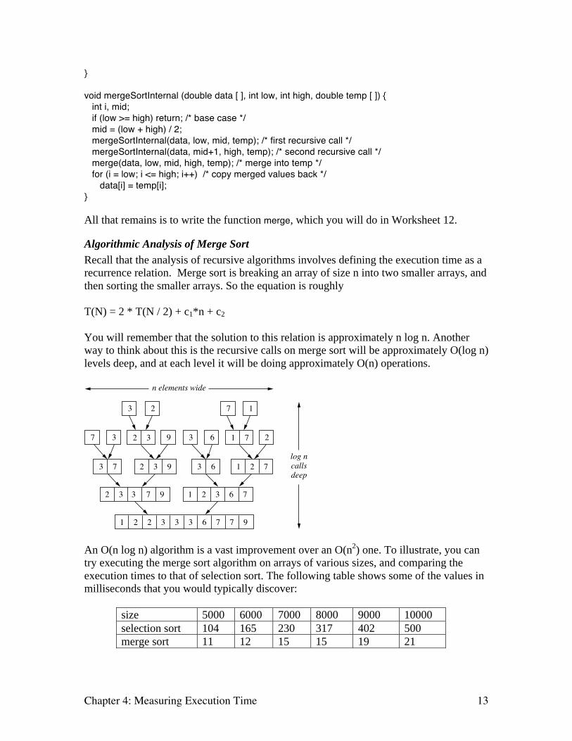
Algorithmic Analysis of Merge Sort

Recall that the analysis of recursive algorithms involves defining the execution time as a

recurrence relation. Merge sort is breaking an array of size n into two smaller arrays, and

then sorting the smaller arrays. So the equation is roughly

T(N) = 2 * T(N / 2) + c1*n + c2

You will remember that the solution to this relation is approximately n log n. Another

way to think about this is the recursive calls on merge sort will be approximately O(log n)

levels deep, and at each level it will be doing approximately O(n) operations.

1 2 2 3 3 3 6 7 7 9

1 2 3 6 7

1 2 72 3 9 3 63 7

2 37 3

3 2 7 1

2 3 3 7 9

9 1 73 6 2

log n calls deep

n elements wide

An O(n log n) algorithm is a vast improvement over an O(n2) one. To illustrate, you can

try executing the merge sort algorithm on arrays of various sizes, and comparing the

execution times to that of selection sort. The following table shows some of the values in

milliseconds that you would typically discover:

size 5000 6000 7000 8000 9000 10000

selection sort 104 165 230 317 402 500

merge sort 11 12 15 15 19 21


Is it possible to do better? The answer is yes and no. It is possible to show, although we

will not do so here, that any algorithm that depends upon a comparison of elements must

have at least an O(n log n) worst case. In that sense merge sort is about as good as we can

expect. On the other hand, merge sort does have one annoying feature, which is that it

uses extra memory. It is possible to discover algorithms that, while not asymptotically

faster than merge sort, do not have this disadvantage. We will examine one of these in the

next section.

Quick Sort

In this section we introduce quick sort. Quick sort, as the name suggests, is another fast

sorting algorithm. Quick sort is recursive, which will give us the opportunity to once

again use the recursive analysis techniques introduced earlier in this chapter. Quick sort

has differing best and worst case execution times, similar in this regard to insertion sort.

Finally, quick sort presents an unusual contrast to the merge sort algorithm.

The quick sort algorithm is in one sense similar to, and in another sense very different

from the merge sort algorithm. Both work by breaking an array into two parts, recursively

sorting the two pieces, and putting them back together to form the final result. Earlier we

labeled this idea divide and conquer.

Where they differ is in the

way that the array is broken

into pieces, and hence the

way that they are put back

together. Merge sort devotes

very little effort to the

breaking apart phase, simply

selecting the first half of the

array for the first list, and the

second half for the second.

This means that relatively

little can be said about the

two sub-arrays, and significant work must be performed to merge them back together.

Quick sort, on the other hand,

spends more time on the task

of breaking apart. Quick sort

selects one element, which is

called the pivot. It then divides

the array into two sections

with the following property:

every element in the first half

is smaller than or equal to the

pivot value, while every

Break

Sort Recursively

Combine

5 9 2 4 7 8 6 12

5 2 4 6 7 9 8 12

2 4 5 6 7 8 9 12

Partition

Sort


element in the second half is larger than or equal to the pivot. Notice that this property

does not guarantee sorting. Each of the smaller arrays must then be sorted (by recursively

calling quick sort). But once sorted, this property makes putting the two sections back

together much easier. No merge is necessary, since we know that elements in the first

part of the array must all occur before the elements in the second part of the array.

Because the two sections do not have to be moved after the recursive call, the sorting can

be performed in-place. That is, there is no need for any additional array as there is when

using the merge sort algorithm. As with the merge sort algorithm, it is convenient to have

the main function simply invoke an interior function that uses explicit limits for the upper

and lower index of the area to be sorted.

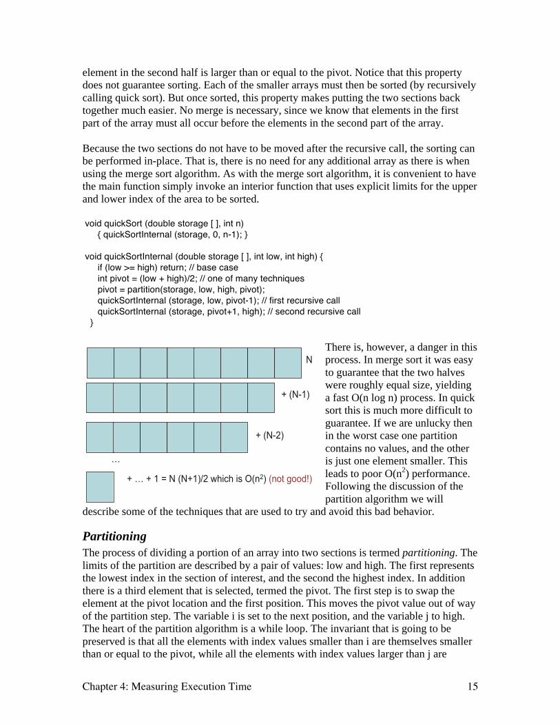
void quickSort (double storage [ ], int n) { quickSortInternal (storage, 0, n-1); } void quickSortInternal (double storage [ ], int low, int high) { if (low >= high) return; // base case int pivot = (low + high)/2; // one of many techniques pivot = partition(storage, low, high, pivot); quickSortInternal (storage, low, pivot-1); // first recursive call quickSortInternal (storage, pivot+1, high); // second recursive call }

There is, however, a danger in this

process. In merge sort it was easy

to guarantee that the two halves

were roughly equal size, yielding

a fast O(n log n) process. In quick

sort this is much more difficult to

guarantee. If we are unlucky then

in the worst case one partition

contains no values, and the other

is just one element smaller. This

leads to poor O(n2) performance.

Following the discussion of the

partition algorithm we will

describe some of the techniques that are used to try and avoid this bad behavior.

Partitioning

The process of dividing a portion of an array into two sections is termed partitioning. The

limits of the partition are described by a pair of values: low and high. The first represents

the lowest index in the section of interest, and the second the highest index. In addition

there is a third element that is selected, termed the pivot. The first step is to swap the

element at the pivot location and the first position. This moves the pivot value out of way

of the partition step. The variable i is set to the next position, and the variable j to high.

The heart of the partition algorithm is a while loop. The invariant that is going to be

preserved is that all the elements with index values smaller than i are themselves smaller

than or equal to the pivot, while all the elements with index values larger than j are

…

N

+ (N-1)

+ (N-2)

+ … + 1 = N (N+1)/2 which is O(n2) (not good!)


themselves larger than the pivot. At each step of the loop the value at the i position is

compared to the pivot. If it is smaller or equal, the invariant is preserved, and the i

position can be advanced:

Pivot <= Pivot Unknown >= Pivot

i j

Otherwise, the location of the j position is compared to the pivot. If it is larger then the

invariant is also preserved, and the j position is decremented. If neither of these two

conditions is true the values at the i and j positions can be swapped, since they are both

out of order. Swapping restores our invariant condition.

The loop proceeds until the values of i and j meet and pass each other. When this happens

we know that all the elements with index values less than i are less than or equal to the

pivot. This will be the first section. All those elements with index values larger than or

equal to i are larger than or equal to the pivot. This will be the second section. The pivot

is swapped back to the top of the first section, and the location of the pivot is returned

Pivot <= Pivot >= Pivot

i

The execution time of quicksort depends upon selecting a good pivot value. Many

heuristics have been proposed for this task. These include

• Selecting the middle element, as we have done

• Selecting the first element. This avoids the initial swap, but leads to O(n2)

performance in the common case where the input is already sorted

• Selecting a value at random

• Selecting the median of three randomly chosen values

From the preceding description you should be able to complete the partition algorithm,

and so complete the quick sort algorithm. You will do this in worksheet 13.

Study Questions

1. What is a linear search and how is it different from a binary search?

2. Can a linear search be performed on an unordered list? Can a binary search?


3. If you start out with n items and repeatedly divide the collection in half, how many

steps will you need before you have just a single element?

4. Suppose an algorithm is O(n), where n is the input size. If the size of the input is

doubled, how will the execution time change?

5. Suppose an algorithm is O(log n), where n is the input size. If the size of the input is


6. Suppose an algorithm is O(n2), where n is the input size. If the size of the input is


7. What does it mean to say that one function dominates another when discussing

algorithmic execution times?

8. Explain in your own words why any sorting algorithm that only exchanges values

with a neighbor must be in the worst case O(n2).

9. Explain in your own words how the shell sort algorithm gets around this limitation.

10. Give an informal description, in English, of how the merge sort algorithm works.

11. What is the biggest advantage of merge sort over selection sort or insertion sort?

What is the biggest disadvantage of merge sort?

12. In your own words given an informal explanation of the process of forming a

partition.

13. Using the process of forming a partition described in the previous question, give an

informal description of the quick sort algorithm.

14. Why is the pivot swapped to the start of the array? Why not just leave it where it is?

Give an example where this would lead to trouble.

15. In what ways is quick sort similar to merge sort? In what ways are they different?

16. What does the quick sort algorithm do if all elements in an array are equal? What is

the big-Oh execution time in this case?


17. Suppose you selected the first element in the section being sorted as the pivot. What

advantage would this have? What input would make this a very bad idea? What would be

the big-Oh complexity of the quick sort algorithm in this case?

18. Compare the partition median finding algorithm to binary search. In what ways are

they similar? In what ways are they different?

Exercises

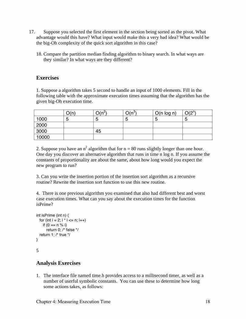
1. Suppose a algorithm takes 5 second to handle an input of 1000 elements. Fill in the

following table with the approximate execution times assuming that the algorithm has the

given big-Oh execution time.

O(n) O(n2) O(n3) O(n log n) O(2n) 1000 5 5 5 5 5 2000 3000 45 10000 2. Suppose you have an n

2 algorithm that for n = 80 runs slightly longer than one hour.

One day you discover an alternative algorithm that runs in time n log n. If you assume the

constants of proportionality are about the same, about how long would you expect the

new program to run?

3. Can you write the insertion portion of the insertion sort algorithm as a recursive

routine? Rewrite the insertion sort function to use this new routine.

4. There is one previous algorithm you examined that also had different best and worst

case execution times. What can you say about the execution times for the function

isPrime?

int isPrime (int n) { for (int i = 2; i * i <= n; i++) if (0 == n % i) return 0; /* false */ return 1; /* true */ } 5

Analysis Exercises

1. The interface file named time.h provides access to a millisecond timer, as well as a

number of userful symbolic constants. You can use these to determine how long

some actions takes, as follows:


# include <time.h> double getMilliseconds( ) { return 1000.0 * clock( ) / CLOCKS_PER_SEC; } int main ( ) { double elapsed; elapsed = getMilliseconds(); … // perform a task elapsed = getMilliseconds() – elapsed; printf(“Elapsed milliseconds = %g\n”, elapsed); } Using this idea write a program that will determine the execution time for selectionSort

for inputs of various sizes. Sort arrays of size n where n ranges from 1000 to 5000 in

increments of 500. Initialize the arrays with random values. Print a table of the input sizes

and execution times. Then plot the resulting values. Does the shape of the curve look like

what you would expect from an n2 algorithm?

2. Recall the function given in the previous chapter that you proved computed an. You

can show that this function takes logarithmic number of steps as a function of n. This

may not be obvious, since in some steps it only reduces the exponent by subtracting one.

First, show that the function takes a logarithmic

number of steps if n is a power of n. (Do you see

why?). Next argue that every even number works by

cutting the argument in half, and so should have this

logarithmic performance. Finally, argue that every

odd number will subtract one and become an even

number, and so the number of times the function is

called with an odd number can be no larger than the number of times it is called with an

even number.

3. A sorting algorithm is said to be stable if the relative positions of two equal elements

are the same in the final result as in the original vector. Is insertion sort stable? Either

give an argument showing that it is, or give an example showing that it is not.

4. Once you have written the merge algorithm for merge sort, provide invariants for your

code and from these produce a proof of correctness.

5. Is merge sort stable? Explain why or why not.

6. Assuming your have proved the partition algorithm correct, provide a proof of

correctness for the quick sort algorithm.

double exp (double a, int n) { if (n == 0) return 1.0; if (n == 1) return a; if (0 == n%2) return exp(a*a, n/2); else return a * exp(a, n-1); }


7. Is quick sort stable?

Programming Projects

1. Experimentally evaluate the running time of Shell Sort versus Insertion sort and

Selection Sort. Are your results similar to those reported here?

2. Experimentally evaluate the running time of Merge sort to that of shell sort and

insertion sort.

3. Rewrite the quick sort algorithm to select a random element in the section being

sorted as the pivot. Empirically compare the execution time of the middle element as

pivot version of quick sort to this new version. Are there any differences in execution

speed?

4. Experimentally compare the execution time of the partition median finding algorithm

to the naïve technique of sorting the input and selecting the middle element. Which

one is usually faster?

On the Web

Wikipedia has an excellent discussion of big-Oh notation and its variations.

The Dictionary of Algorithms and Data Structures provided by the National Institute of

Standards and Technology (http://www.nist.gov/dads/) has entries on binary and linear

search, as well as most other standard algorithms.

The standard C library includes a version of quick sort, termed qsort. However, the

interface is clumsy and difficult to use.

chapter 4: measuring execution time - college of...

Documents