chapter 4 labor market equilibrium copyright © 2010 by the mcgraw-hill companies, inc. all rights...
TRANSCRIPT

Chapter 4
Labor Market Equilibrium
Copyright © 2010 by The McGraw-Hill Companies, Inc. All rights reserved.
McGraw-Hill/Irwin

4-2
Introduction• Labor market equilibrium coordinates the
desires of firms and workers, determining the wage and employment observed in the labor market.
• Market types:– Monopsony: one buyer of labor– Monopoly: one seller of labor
• These market structures generate unique labor market equilibria.
4-3
Equilibrium in a Single Competitive Labor Market
• Competitive equilibrium occurs when supply equals demand, generating a competitive wage and employment level.
• It is unlikely that the labor market is ever in an equilibrium, since supply and demand are dynamic.
• The model suggests that the market is always moving toward equilibrium.

4-4
(Pareto) Efficiency• Pareto efficiency exists when all possible
gains from trade have been exhausted.
• When the state of the world is Pareto Efficient, to improve one person’s welfare necessarily requires decreasing another person’s welfare.
• In policy applications, ask whether a change can make any one better off without harming anyone else. If the answer is yes, then the proposed change is said to be “Pareto-improving”.

4-5
Equilibrium in a Competitive Labor Market
S
D0
w*
P
Q
E* EHEL
Dollars
Employment
The labor market is in equilibrium when supply equals demand; E* workers are employed at a wage of w*. In equilibrium, all persons who are looking for work at the going wage can find a job. The triangle P gives the producer surplus; the triangle Q gives the worker surplus. A competitive market maximizes the gains from trade, or the sum P + Q.

4-6
Efficiency Revisited• The “single wage” property of a competitive
equilibrium has important implications for economic efficiency.
• The allocation of workers to firms that equates the value of marginal product across markets is also the sorting that leads to an efficient allocation of labor resources.

4-7
Competitive Equilibrium in Two Labor Markets Linked by Migration
Suppose the wage in the northern region (wN) exceeds the wage in the southern region (wS). Southern workers want to move North, shifting the southern supply curve to the left and the northern supply curve to the right. In the end, wages are equated across regions at w*.
SS
Dollars
Employment
SS
w*
wS
DS
(b) The Southern Labor Market
Dollars
Employment
SN
wN
w*
DN
(a) The Northern Labor Market
s
A
B
C
4-8
Payroll Taxes and Subsidies• Payroll taxes assessed on employers lead
to a downward, parallel shift in the labor demand curve.– The new demand curve shows a wedge between the
amount the firm must pay to hire a worker and the amount that workers actually receive.
– Payroll taxes increase total costs of employment, so these taxes reduce employment in the economy.
– Firms and workers share the cost of payroll taxes, since the cost of hiring a worker rises and the wage received by workers declines.
– Payroll taxes result in deadweight losses.
4-9
Employment
B
Dollars
w1 + 1
w0
S
D0
D1
w1
w0 1
E1 E0
A
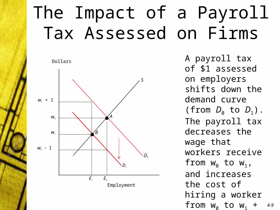
The Impact of a Payroll Tax Assessed on Firms
A payroll tax of $1 assessed on employers shifts down the demand curve (from D0 to D1). The payroll tax decreases the wage that workers receive from w0 to w1, and increases the cost of hiring a worker from w0 to w1 + 1.

4-10
The Impact of a Payroll Tax Assessed on Workers
Dollars
w1
w0
S0
D0
D1
D0
E1 E0 Employment
S1
w0 + 1
w1 1
A payroll tax assessed on workers shifts the supply curve to the left (from S0 to S1). The payroll tax has the same impact on the equilibrium wage and employment regardless of who it is assessed on.
4-11
Payroll Subsidies
• An employment subsidy lowers the cost of hiring for firms.
• This means payroll subsidies shift the demand curve for labor to the right (up).
• Total employment will increase as the cost of hiring has fallen.
4-12
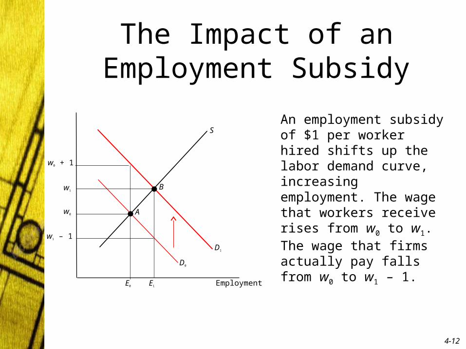
The Impact of an Employment Subsidy
An employment subsidy of $1 per worker hired shifts up the labor demand curve, increasing employment. The wage that workers receive rises from w0 to w1. The wage that firms actually pay falls from w0 to w1 – 1.
w1
S
D1
D0
w0
E0 E1
B
A
Employment
w0 + 1
w1 – 1

4-13
Immigration
• As immigrants enter the labor market, the labor supply curve shifts to the right.– Total employment increases.– Equilibrium wage decreases.

4-14
The Short-Run Impact of Immigration When Immigrants and
Natives Are Perfect SubstitutesDollars
Supply
w0
w1
Demand
N0EmploymentE1N1
As immigrants and natives are perfect substitutes, the two groups are competing in the same labor market. Immigration shifts out the labor supply curve. As a result, the wage falls from w0 to w1, and total employment increases from N0 to E1. At the lower wage, the number of natives who work declines from N0 to N1.

4-15
The Short-Run Impact of Immigration when Immigrants and
Natives are Complements
w1
w0
Dollars
Supply
Demand
N1N0Employment
If immigrants and natives are complements, they do not compete in the same labor market. The labor market here denotes the supply and demand for native workers. Immigration makes natives more productive, shifting out the labor demand curve. This leads to a higher native wage and to an increase in native employment.
4-16
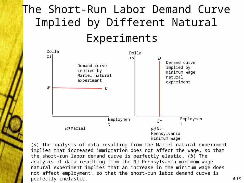
The Short-Run Labor Demand Curve
Implied by Different Natural Experiments Dollars Dollars
EmploymentE*Employment
(b) NJ-Pennsylvania minimum wage
(a) Mariel
w*
D
Demand curve implied by Mariel natural experiment
D
Demand curve implied by minimum wage natural experiment
(a) The analysis of data resulting from the Mariel natural experiment implies that increased immigration does not affect the wage, so that the short-run labor demand curve is perfectly elastic. (b) The analysis of data resulting from the NJ-Pennsylvania minimum wage natural experiment implies that an increase in the minimum wage does not affect employment, so that the short-run labor demand curve is perfectly inelastic.

4-17
The Cobweb Model
• Two assumptions of the cobweb model:– Time is needed to produce skilled workers.– Persons decide to become skilled workers by
looking at conditions in the labor market at the time they enter school.
• A “cobweb” pattern forms around the equilibrium.

4-18
Cobweb Model (continued)
• The model assumes naïve workers who do not form rational expectations.
• Rational expectations are formed if workers correctly perceive the future and understand the economic forces at work.

4-19
Noncompetitive Labor Markets: Monopsony
• Monopsony market exists when a firm is the only buyer of labor.
• Monopsonists must increase wages to attract more workers.
• Two types of monopsonist firms:– Perfectly discriminating– Nondiscriminating

4-20
Wage and employment determination under a monopsony labor market
4-21
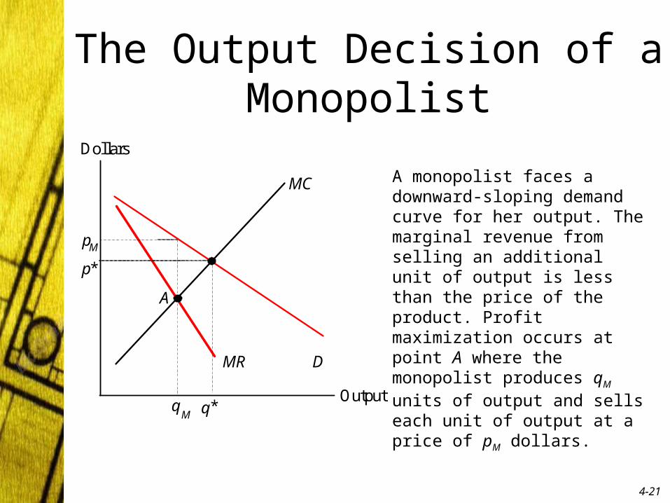
The Output Decision of a Monopolist
Dollars
Output
p
MC
D
*
MR
q *
p M
q M
A
A monopolist faces a downward-sloping demand curve for her output. The marginal revenue from selling an additional unit of output is less than the price of the product. Profit maximization occurs at point A where the monopolist produces qM units of output and sells each unit of output at a price of pM dollars.
4-22
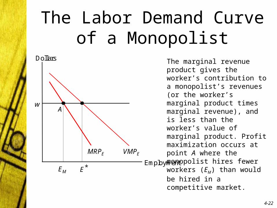
The Labor Demand Curve of a Monopolist
Dollars
Employment
w
MRPE VMPE
EM E*
A
The marginal revenue product gives the worker’s contribution to a monopolist’s revenues (or the worker’s marginal product times marginal revenue), and is less than the worker’s value of marginal product. Profit maximization occurs at point A where the monopolist hires fewer workers (EM) than would be hired in a competitive market.

4-23
End of chapter 4