90

Chapter 4 Field Study of CFC Concentrations at the

Water Table at the Mirror Lake Site, New

Hampshire

4.1 Introduction

4.1.1 CFCÕs as Environmental Tracers

Chlorofluorocarbons (CFC's; also called Freon, chlorofluoromethane) have

emerged as useful age-dating tracers for young ground water (Thompson et al., 1974;

Thompson and Hayes, 1979; Plummer et al., 1993). For atmospheric tracers, the age of

ground water is defined as the time since the water was in contact with the atmosphere.

Conceptually, recharge to the saturated zone is in chemical equilibrium with the

atmosphere at the water table, and below in the saturated zone that concentration is

maintained. Hence, if the atmospheric concentration changes in time, then different

concentrations in ground water presumably correspond to different recharge times, and

different ages. Knowledge of the atmospheric source term allows calibration of flow and

transport models, yielding estimates of hydraulic and transport properties (e.g. Reilly et

al., 1994; Szabo et al., 1996). These methods are most useful where the flow system

under investigation is too large or responds too slowly to test through traditional field

tracer experiments.

CFCÕs are useful ground-water tracers because the atmospheric source term is

relatively well known and is almost linear in time, and because the CFC concentration of

fresh water in equilibrium with the atmosphere is well described as a function of

temperature alone (Warner and Weiss, 1985; Bu and Warner, 1995). CFC-12, CFC-11,

and CFC-113 are man-made volatile organic compounds widely used as refrigerants and

91

occurring in many manufactured goods. The atmospheric concentration of CFCÕs has

been increasing since their creation in the 1940Õs (fig. 4-1). Atmospheric concentrations

have been measured for approximately 30 years and concentrations before 1960 are

estimated from manufacturing records. Recently, concentrations of CFCÕs have leveled

off and in the case of CFC-11 and CFC-113 have begun to decrease somewhat due to

reduced production, atmospheric loss (by reaction) and transfer of CFCÕs from the

atmosphere to the oceans (Khalil and Rasmussen, 1993).

0

100

200

300

400

500

600

AT

MO

SP

HE

RIC

CO

NC

EN

TR

AT

ION

(p

ptv)

CFC-12

CFC-11

CFC-113

1940 1950 1960 1970 1980 1990 2000

~ 1 pptv

12 11 113

Figure 4-1. Global atmospheric concentration of CFC-12, CFC-11, and CFC-113 (after

Plummer et al., 1993)

Assuming that recharging ground water is in CFC equilibrium with the

atmosphere, a measured CFC concentration in water can be converted to a corresponding

atmospheric concentration, which in turn can be used to compute a corresponding date of

recharge from Figure 4-1. The difference between the date of recharge and the date of

sampling is the age of the ground water.

92

The dating of ground water from CFCÕs depends, in part, on the assumption that

CFCÕs are inert; once isolated from the atmosphere, the CFC concentration in a moving

volume of water is constant in time. Processes which may change CFC concentrations

include mixing and dispersion, exchange with solids, gases, or immobile waters, and

degradation by biotic or abiotic reactions (Busenberg and Plummer, 1992). Degradation

of CFCÕs in water has been identified for anaerobic conditions (Khalil and Rasmussen,

1989; Lovely and Woodward, 1992; Semprini et al., 1990; Terauds et al., 1993; Bullister

and Lee, 1995; Oster et al., 1996; Plummer et al., in press). However, in oxygenated

waters CFCÕs appear to be essentially inert. Furthermore, the relatively linear increase in

the atmospheric concentrations over time means that CFC concentrations are less affected

by mixing and dispersion than tracers with highly variable source terms, such as tritium

(Plummer et al., 1993). Exchange processes may be important for CFCÕs, especially in

highly heterogeneous formations, such as fractured rock (Shapiro, 1996; Wood et al.,

1996). Sorption of CFCÕs to most natural aquifer materials is believed to be insignificant

(Russell and Thompson, 1983; Lovely and Woodward, 1992). Despite these beneficial

factors, CFC concentrations in ground water are not always easy to interpret. The U.S.

Geological Survey Mirror Lake, New Hampshire site is one location where CFCÕs have

not been as useful as hoped in characterizing large-scale transport properties (Busenberg

and Plummer, 1996; Shapiro et al., 1996).

4.1.2 Mirror Lake Field Site

The U.S. Geological Survey (USGS) is investigating multi-scale flow and

transport in a glaciated fractured rock setting at the Mirror Lake site, Grafton County,

New Hampshire (fig. 4-2) (Winter, 1984; Shapiro and Hsieh, 1991; Hsieh et al., 1993).

These investigations are multi-disciplinary and use tools ranging from detailed geologic

and fracture mapping, to surface seismic and borehole radar, to crosshole hydraulic and

tracer tests (Hsieh and Shapiro, 1996) and large-scale flow model calibration (Tiedeman

et al., 1997). Ground water from both the fractured bedrock and from the overlying

93

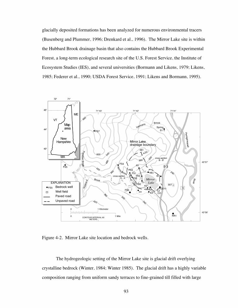
glacially deposited formations has been analyzed for numerous environmental tracers

(Busenberg and Plummer, 1996; Drenkard et al., 1996). The Mirror Lake site is within

the Hubbard Brook drainage basin that also contains the Hubbard Brook Experimental

Forest, a long-term ecological research site of the U.S. Forest Service, the Institute of

Ecosystem Studies (IES), and several universities (Bormann and Likens, 1979; Likens,

1985; Federer et al., 1990; USDA Forest Service, 1991; Likens and Bormann, 1995).

K2

MirrorLake

71°42'

Mirror Lakedrainage boundary

71°41'71°43'

600

481

43°56'

43°57'

0 1 Kilometer

0 1 MileCONTOUR INTERVAL 60

METERS

71°72°

43°

44°

45°

NewHampshire

Map-area

VT

ME

MA

Paved road

Unpaved road

Well field

Bedrock wellEXPLANATION

IS1

H1

R1

TR1TR2

T1

FS5FS4

FS3FS1

FS6 CO11K1

K3

FS5307

9 3

3

RR1

FS7 S1Spring

cross-section-A - A'

cross-section-B - B'

FS2

FSE

CO

Norris Brook

Paradise B

rook

Pem

ige wa sset

River

Hub

bard

Brook

360 300

Leemans Brook

240420

240

300

420

360

540

480

420

360

660

Figure 4-2. Mirror Lake site location and bedrock wells.

The hydrogeologic setting of the Mirror Lake site is glacial drift overlying

crystalline bedrock (Winter, 1984; Winter 1985). The glacial drift has a highly variable

composition ranging from uniform sandy terraces to fine-grained till filled with large

94

boulders (Winter, 1984; Harte, 1992; Harte and Winter, 1996). The permeability of the

glacial drift is generally low (Wilson, 1991; Harte, 1997). Regional-scale flow modeling

indicates that the transmissivities of the glacial drift and the underlying fractured bedrock

are low and of the same order of magnitude (Tiedeman et al., 1997). Baseflow to streams

in the Mirror Lake drainage basin is significantly higher than in other parts of the

Hubbard Brook drainage basin because of the increased thickness of glacial drift (Winter

et al., 1989; Mau and Winter, 1997). Sandy terrace deposits located throughout the

watershed may have strong local control on ground-water flow and ground-water/surface

water interaction (Shattuck, 1991; Harte and Winter, 1996). The climate is humid and

long-term average recharge to ground water is on the order of 30 cm/yr (Mau and Winter,

1997).

4.1.3 Ground-Water Ages from CFC Data at Mirror Lake

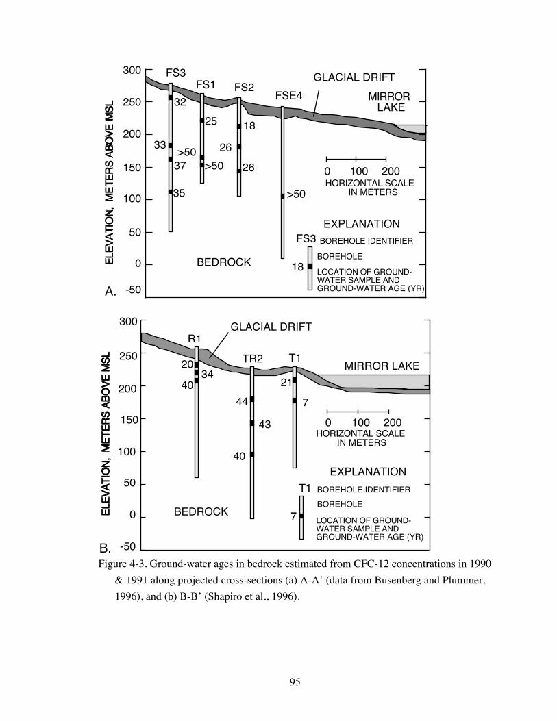
In contrast to results from some relatively homogeneous coastal plain sediments

(e.g. Reilly et al., 1994; Szabo et al., 1996), ground-water ages derived from CFC

concentrations in samples from site bedrock wells do not follow a readily apparent spatial

distribution. Figure 4-3 shows cross-sections of ground-water ages determined from

samples collected from packer-isolated portions of open bedrock boreholes at the Mirror

Lake site (Busenberg and Plummer, 1996; Shapiro et al., 1996). In homogeneous

formations, ground-water age is expected to increase gradually from recharge to

discharge locations, as shown in Chapter 2. However, in the highly heterogeneous

fractured rock at Mirror Lake, in which the small-scale hydraulic conductivity varies over

at least 7 orders of magnitude (Hsieh and Shapiro, 1996), complex patterns such as those

shown in Figure 4-3 may be expected. This is consistent with ground-water age

simulation results shown in, for example, Figure 2-8.

95

ELE

VA

TIO

N,

ME

TE

RS

AB

OV

E M

SL

ELE

VA

TIO

N,

ME

TER

S A

BO

VE

MS

L

300

250

200

150

100

50

0

-50

FS3FS1 FS2

FSE4 MIRROR- LAKE

GLACIAL DRIFT

BEDROCK

0 100 200

7

7

21

43

40

44

2034

40

HORIZONTAL SCALE-IN METERS

T1

R1

TR2 T1

BEDROCK

BOREHOLE IDENTIFIER

BOREHOLE

LOCATION OF GROUND--WATER SAMPLE AND-GROUND-WATER AGE (YR)

300

250

200

150

100

50

0

-50

ELE

VA

TIO

N,

ME

TE

RS

AB

OV

E M

SL

GLACIAL DRIFT

MIRROR LAKE

EXPLANATION

ELE

VA

TIO

N,

ME

TE

RS

AB

OV

E M

SL

0 100 200

18

HORIZONTAL SCALE-IN METERS

FS3 BOREHOLE IDENTIFIER

BOREHOLE

LOCATION OF GROUND--WATER SAMPLE AND-GROUND-WATER AGE (YR)

EXPLANATION

A.

B.

32

33

37

35

>50>50

25 18

26

26

>50

Figure 4-3. Ground-water ages in bedrock estimated from CFC-12 concentrations in 1990

& 1991 along projected cross-sections (a) A-AÕ (data from Busenberg and Plummer,

1996), and (b) B-BÕ (Shapiro et al., 1996).

96

Other possible causes of the complex age spatial pattern at Mirror Lake, and the

corresponding CFC concentration pattern, involve in situ processes that modify CFC

concentrations. Possible processes include, but may not be limited to, sorption,

exchange, and degradation. Furthermore, seasonal temperature cycles may cause

corresponding cycles in CFC concentrations in recharging waters (Chapter 3). These

cycles may lead to variability in CFC concentrations along a flow path that may be

misinterpreted as highly variable ages. Previous and concurrent work indicates that

CFCÕs, particularly CFC-11 and CFC-113, are degraded under anaerobic conditions in

ground water (Semprini et al., 1990; Terauds et al., 1993; Plummer et al., in press).

4.1.4 Scope and Objectives

The goals of this field study are to characterize the concentrations of CFCÕs in

water recharging the saturated zone at Mirror Lake, to identify the processes that control

those concentrations, and to describe the source function for CFCÕs in infiltrating waters

that recharge the saturated zone. The field program investigates the following properties

and processes: CFC concentrations at or near the water table, and in the unsaturated zone;

temperature cycles where CFC air/water equilibrium is occurring; biogeochemical factors

that may be related to CFC concentrations; and hydraulic properties of the unsaturated

zone. Section 4.2 describes methods used in this field study, and results are presented in

section 4.3. These results are discussed and processes controlling CFC in recharge water

at the Mirror Lake site are identified in section 4.4. Preliminary summaries of the

findings here have been presented at scientific meetings (see abstacts: Goode, 1997;

Goode et al., 1997).

97

4.2 Methods

Some of the data used in this study were obtained from previous and ongoing

research at Mirror Lake and at Hubbard Brook Experiment Forest conducted by U.S.

Forest Service, Institute of Ecosystems Studies (IES), U.S. Geological Survey, and

numerous universities. Geochemical data, including CFC results from bedrock wells and

isolated piezometers were provided by USGS. Water level measurements are also

provided by USGS and IES. Barometric pressure data were provided by IES.

Precipitation and air temperature data were provided by USFS, Radnor Pa. Hydrogen

concentrations in water reported here were provided by USGS (Don A. Vroblesky,

written communication, 1997).

4.2.1 Moisture Content and Pressure

Unsaturated zone hydraulic conditions were monitored during 1996 and 1997,

with most data collected during the summers. A Time-Domain-Reflectometry (TDR)

system from CSI and Tektronix was used to measure soil moisture near W2 (fig. 4-4).

The system consists of a CR10 datalogger with special TDR PROM chips, a Tektronix

1502B cable tester, a CSI multiplexer, coax cable, and CSI model 605 3-rod TDR probes.

TDR measures the reflection time of an electrical pulse, which is a function of the

moisture content around the 3-rod 30-cm probe. The measurement is the average

moisture content within an elliptical cylinder 30 cm long, about 10 cm maximum cross-

section and about 5 cm minimum cross-section. One of the first long-term field

applications of automated TDR was performed at Hubbard Brook Experimental Forest by

Herkelrath and others (1991).

Soil suction pressure head was measured at four depths near the TDR system,

near W2. Soil Moisture Inc. tensiometers were used with depths of approximately 30, 60,

and 90 cm. These tensiometers consist of a porous ceramic cup at the end of a clear

plastic rigid tube of the appropriate length. A calibrated pressure gage in installed near

98

the top of the tensiometer, and a water reservoir with Ôquick-fillÕ system is mounted on

the top. The gage reading was recorded periodically by field personnel.

A secondary automatic measure of soil suction pressure head was obtained during

the last part of this study using gypsum blocks. These gypsum blocks were also installed

near the TDR system, near W2. Gypsum blocks were installed at depths ranging from 10

to 90 cm. The CSI datalogger of the TDR system was additionally programmed to

measure the electrical resistance of the gypsum blocks which is a function of the moisture

content in the block. The blockÕs moisture content depends in turn on the prevailing soil

pressure head in the surrounding material. These gypsum blocks were not calibrated in

the laboratory and give only qualitative measures of pressure, but were used because the

measurements are continuous, and supplement the direct tensiometer measurements.

Well water levels were measured throughout this study using manual electrical

tape, and using continuous pressure transducer measurements. The water level indicator

used was a Slope Indicator Inc. model 51453 which is marked in 0.01 ft (about 0.3 cm)

intervals. Druck submersible pressure transducers were used with CSI dataloggers, and

these were continuously calibrated in the field from manual water level measurements.

4.2.2 Soil Temperature

Average hourly soil temperature was monitored from June 1996 through

September 1997 at several depths at two locations in the study area: near the FS3 and

FS3C well clusters, and near FS4 and FS4-WT. Campbell Scientific Inc. (CSI) model

107B soil temperature probes were installed in natural backfill in hand augered

boreholes. The average hourly temperature was recorded from measurements made

every 5 minutes. Data collection was automated with CSI CR10 dataloggers. At the

FS3C site, one temperature probe was installed in the bottom of piezometer FS3C-14,

which was dry throughout the monitoring period. At each location, a CSI model 107U air

temperature probe was installed on the ground in a small plastic box. At the FS3C site,

99

the depths of measurement of soil temperature were 0, 0.8 m, 1.9 m, and 3.5 m. At the

FS4 site, the measurements depths were 0, 42 cm and 75 cm.

4.2.3 Water Sample Collection and Analysis

Water samples were collected from 31 shallow piezometers during the summers

of 1995, 1996, and 1997. Figure 4-4 shows the locations of these wells within the Mirror

Lake watershed, Grafton County, New Hampshire. These wells were constructed by the

U.S. Geological Survey over approximately 20 years as part of ground-water/lake

interaction studies (Winter, 1984) and of fractured rock research (Shapiro and Hsieh,

1996). Wells are constructed of either steel or PVC (Table 4-1) and are almost all

screened over 0.6 to 0.9 m long intervals. This sampling effort focused primarily on

wells screened near the water table, but also included some wells screened in the glacial

drift beneath the water table. New wells constructed for the present study are W16A,

W33, W34, W35, W36, and FS4-WT. These wells were installed by the USGS New

Hampshire District drill rig crew under supervision by the author. These boreholes were

power augered without adding any water during drilling, and the wells were constructed

of threaded PVC to minimize CFC contamination. Except where the borehole caved

during auger withdrawal, coarse sand was placed in the annulus around the screen,

followed by natural backfill, followed by a layer of ground silica flour, and natural

backfill to the surface. The purpose of the fine-grained ground silica is to minimize

vertical flow within the borehole annulus.

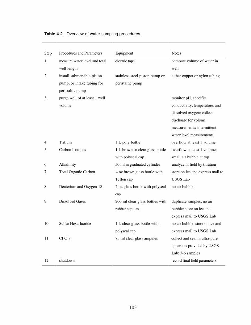
The general procedures for sampling (Table 4-2) consisted of pumping at least 1

borehole volume and then collecting water samples using standard procedures and

equipment developed by USGS. CFC samples were collected using procedures and

equipment developed at the USGS CFC Lab, Reston Virginia (Busenberg and Plummer,

1992).

100

260300 R1

TR2

FS2

FS1

FS3

W27

W25

W3,3A

W34

W33

W2

W15

W16,16A

W36

W35

W26

S3

0

0

100 meters

300 feet

71°42'

LANDSURFACE ELEVATION-IN METERS (VARIABLEINTERVAL)-

ROAD-

PIEZOMETER-

WELL CLUSTER-

SEEP

W25

FS2

S1

43°56'40"

43°56'50"

71°41'50"71°42'10"

HQ

260300

FS3C

S40

240

W Stream

Figure 4-4. Locations of individual piezometers, well clusters, and seep sampled for this

study.

101

Table 4-1. Selected piezometer construction data. [Primary references: W84, Winter, 1984; W94, T.C. Winter, personal commun., 1995; H91,

P.T. Harte, written commun., 1991; H97, Harte, 1997; S91, Shattuck, 1991]

Well ID Date installed Casingmaterial

Casing Diam.(cm)

Screen type Screen Length(cm)

Screen topdepth (m)

Top of casingelevation (m)

Land surfaceelevation (m)

Primary reference

W2 Nov-78 PVC 5.1 PVC wound 91 4.6 256.78 W84W3 Nov-78 PVC 3.2 PVC slotted 76 5.9 258.56 W84W3A Nov-78 PVC 5.1 PVC slotted 76 1.7 259.11 W84W6 Jul-82 Steel 5.1 Steel wound 91 9.4 239.27 W84W11 Jul-82 ABS 5.1 PVC wound 61 7.3 240.97 240.1 W84W15 Jul-82 Steel 3.2 Steel wound 91 0.9 263.26 W84W16 Jul-82 Steel 3.2 Steel wound 91 5.5 264.82 W84W16A Jul-96 PVC 5.1 PVC wound 61 2.1 263.8 this studyW25 Oct-88 PVC 5.1 PVC wound 61 6.7 262.34 261.0 W94W26 Oct-88 PVC 5.1 PVC wound 61 4.9 258.05 256.8 W94W27 Aug-90 PVC 5.1 PVC slotted 152 4.9 266.93 265.9 H91W33 Jul-96 PVC 5.1 PVC wound 61 5.2 256.0 this studyW34 Jul-96 PVC 5.1 PVC wound 61 4.5 258.0 this studyW35 Jul-96 PVC 5.1 PVC wound 61 2.4 271.0 this studyW36 Jul-96 PVC 5.1 PVC wound 61 5.2 272.0 this studyFS1-17 Jul-82 Steel 5.1 Steel wound 91 4.9 262.64 261.3 W84FS1-25 Aug-79 PVC 5.1 PVC wound 61 6.9 262.35 261.2 W94FS1-35 Aug-79 PVC 5.1 PVC wound 61 9.5 262.22 260.7 W94FS3-11 PVC 5.1 61 2.7 275.04 274.0FS3-22 PVC 5.1 61 6.1 275.05 274.0FS3-29 PVC 5.1 61 8.2 275.02 274.0FS3C-14 Aug-91 PVC 5.1 PVC slotted 15 3.9 273.81 273.6 H97FS3C-19 Aug-91 PVC 5.1 PVC slotted 15 5.5 274.27 273.7 H97FS3C-24 Aug-91 PVC 5.1 PVC slotted 15 7.2 274.32 273.7 H97FS3C-29 Aug-91 PVC 5.1 PVC slotted 15 8.8 274.13 273.7 H97FS4-WT Jul-96 PVC 5.1 PVC wound 61 1.1 349.7 this studyR1-36 Aug-90 PVC 5.1 PVC slotted 152 9.6 257.30 256.5 H91R1-55 PVC 5.1 61 15.5 257.32 256.2S40 Aug-88 PVC 5.1 PVC slotted 24 0.5 255.30 254.3 S91T1-8 Jul-82 Steel 5.1 Steel wound 91 1.5 229.62 228.9 W84TR1-63 Sep-83 PVC 5.1 PVC wound 183 17.4 249.30 248.4 W94

103

Table 4-2. Overview of water sampling procedures.

Step Procedures and Parameters Equipment Notes

1 measure water level and total

well length

electric tape compute volume of water in

well

2 install submersible piston

pump, or intake tubing for

peristaltic pump

stainless steel piston pump or

peristaltic pump

either copper or nylon tubing

3. purge well of at least 1 well

volume

monitor pH, specific

conductivity, temperature, and

dissolved oxygen; collect

discharge for volume

measurements; intermittent

water level measurements

4 Tritium 1 L poly bottle overflow at least 1 volume

5 Carbon Isotopes 1 L brown or clear glass bottle

with polyseal cap

overflow at least 1 volume;

small air bubble at top

6 Alkalinity 50 ml in graduated cylinder analyze in field by titration

7 Total Organic Carbon 4 oz brown glass bottle with

Teflon cap

store on ice and express mail to

USGS Lab

8 Deuterium and Oxygen-18 2 oz glass bottle with polyseal

cap

no air bubble

9 Dissolved Gases 200 ml clear glass bottles with

rubber septum

duplicate samples; no air

bubble; store on ice and

express mail to USGS Lab

10 Sulfur Hexafluoride 1 L clear glass bottle with

polyseal cap

no air bubble, store on ice and

express mail to USGS Lab

11 CFCÕs 75 ml clear glass ampules collect and seal in ultra-pure

apparatus provided by USGS

Lab; 3-6 samples

12 shutdown record final field parameters

104

Field water quality parameters included temperature, pH, specific

conductivity, dissolved oxygen, and alkalinity. Specific conductivity and pH were

measured with separate Orion probes , both of which also measured temperature.

In some cases the probes were lowered into the piezometer prior to sampling to

record in s itu values . Dissolved oxygen was measured in the field us ing the

Winkler titration method (Hach kit) or a YSI self-s tirring BOD probe (model

5905). Alkalinity was measured us ing 0.16 N sulfuric acid titration of 50 ml

samples . Collected samples were analyzed at the following USGS laboratories :

CFC Lab and Isotope Lab in Res ton; National Water Quality Lab in Denver; and

Tritium Lab in Menlo Park.

4.2.4 Soil Gas Sampling and Analys is

Soil gas samples were collected during the summers of 1996 and 1997, and

in January 1997 from s teel dry wells installed by hand or power auger, or manual

drive point in one case (fig. 4-5; Table 4-3). Figure 4-6 shows a schematic of the

a s teel gas well cons is ting of 0.6 cm diameter s tainless s teel tubing, stainless s teel

or brass swagelok compression fittings , a s tainless steel screen, and glass wool.

The borehole annulus around the sampling port is filled with coarse sand,

followed by natural backfill, followed by ground s ilica flour, and natural backfill

to the surface.

105

300 R1

TR2

FS2

FS1

FS3

W27

W25W3,3A

W34

W33

W2

W15

W16,16A

W36

W35

W26

S3

0

0

100 meters

300 feet

71°42'

LANDSURFACE ELEVATION-IN METERS (VARIABLEINTERVAL)-

ROAD-

PIEZOMETER-

WELL CLUSTER-

SEEP-

SOIL GAS TUBES

W3

FS2

S3

43°56'40"

43°56'50

71°41'50"71°42'10"

HQ

FS3C

S40

300

240

FS3 (red,blue)

FS3T

W2

260

W Stream

Figure 4-5. Locations of soil gas sampling tubes installed for this study.

106

stainless steel tubingvariable length0.6 cm diameter(1/4 inch)

coarse sand

swagelokcompressionfittings andstainlesssteel screen

natural backfill

natural backfill

slotted stainlesssteel tubing filledwith glass wool~ 10 cm length(4 inches)

silica flour

hand augered (10 cm)or power augered (20 cm)borehole

Figure 4-6. Schematic of typical soil gas well.

Soil gas samples were pumped from the dry well into glass ampules which were

sealed by welding. A Rasmussen stainless steel gas pump with Teflon diaphragm (40

psig model) was attached to the dry well and pumped for 2-3 minutes to purge the well.

All metal (aluminum and stainless steel) tubing was used. Samples were collected after

purging in 150 ml glass ampules which were sealed by welding the ampule neck closed

with a MAP gas torch. Three samples were normally collected from each dry well. All

CFC gas samples were analyzed at the USGS CFC Lab in Reston.

107

Air samples were also collected to ascertain the local CFC gas concentrations.

Samples were collected using the Rasmussen pump with aluminum tubing and a stainless

steel cylinder provided by the USGS CFC Lab in Reston. Additional samples were

collected using the same apparatus and sample ampules as the soil gas, but with the pump

intake in air, 1-2 m above ground. These samples provide further information on local

CFC air concentrations, and possible sample apparatus contamination.

108

4.3 Results

4.3.1 Moisture Content and Pressure

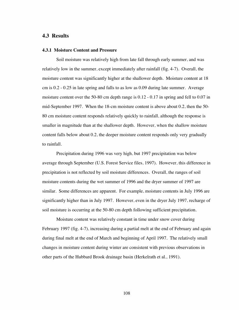
Soil moisture was relatively high from late fall through early summer, and was

relatively low in the summer, except immediately after rainfall (fig. 4-7). Overall, the

moisture content was significantly higher at the shallower depth. Moisture content at 18

cm is 0.2 - 0.25 in late spring and falls to as low as 0.09 during late summer. Average

moisture content over the 50-80 cm depth range is 0.12 - 0.17 in spring and fell to 0.07 in

mid-September 1997. When the 18-cm moisture content is above about 0.2, then the 50-

80 cm moisture content responds relatively quickly to rainfall, although the response is

smaller in magnitude than at the shallower depth. However, when the shallow moisture

content falls below about 0.2, the deeper moisture content responds only very gradually

to rainfall.

Precipitation during 1996 was very high, but 1997 precipitation was below

average through September (U.S. Forest Service files, 1997). However, this difference in

precipitation is not reflected by soil moisture differences. Overall, the ranges of soil

moisture contents during the wet summer of 1996 and the dryer summer of 1997 are

similar. Some differences are apparent. For example, moisture contents in July 1996 are

significantly higher than in July 1997. However, even in the dryer July 1997, recharge of

soil moisture is occurring at the 50-80 cm depth following sufficient precipitation.

Moisture content was relatively constant in time under snow cover during

February 1997 (fig. 4-7), increasing during a partial melt at the end of February and again

during final melt at the end of March and beginning of April 1997. The relatively small

changes in moisture content during winter are consistent with previous observations in

other parts of the Hubbard Brook drainage basin (Herkelrath et al., 1991).

108109

0.05

0.1

0.15

0.2

0.25

0.3

0.35

6/1 8/1 10/1 12/1 1/31 4/2 6/2 8/20.05

0.1

0.15

0.2

0.25

0.3

0.35

VO

LUM

ET

RIC

WA

TE

R C

ON

TE

NT

1996

18 cm

50-80 cm

1997

10/1

Figure 4-7. Moisture content during 1996 and 1997 near W2 at depth of 18 cm and

average over depth range 50-80 cm.

Tensiometer measurements of pressure head in the unsaturated zone are similar to

the soil moisture results, although tensiometer results are available only for the summers

of 1996 and 1997 (fig 4-8). Suction head (negative pressure head) is low in the early

summer at all depths but increases significantly at the 30 cm depth as the upper soil zone

dries out. Fluctuations in suction head at 30 cm generally mirror soil moisture

fluctuations, with high moisture content and low suction head after rainfall, and then

falling moisture content and increasing suction head as drying proceeds. The deeper 60-

and 90-cm suction pressure heads changed much less during the monitored period. The

90-cm results were essentially constant in the range 10-14 centibars, while the 60-cm

suction head increased somewhat only after extended drying, and then increased only to

about 30 centibars.

110

0

10

20

30

40

50

60

70

806/15 6/30 7/16 7/31 8/16 9/1

SU

CT

ION

PR

ES

SU

RE

HE

AD

(cm

H20

)

1996

90 cm

60 cm

30 cm

a .

0

10

20

30

40

50

60

70

806/1 6/16 7/1 7/16 7/31 8/15 8/30 9/15

SU

CT

ION

PR

ES

SU

RE

HE

AD

(cm

H 2

0)

1997

90 cm

60 cm

30 cm

b .

Figure 4-8. Suction pressure head at W2 TDR site during (a) the summer of 1996, and

(b) the summer of 1997.

111

Although uncalibrated, the gypsum block results provide a continuous record of

relative fluctuations of suction pressure head during the summer of 1997. The 3 blocks

installed with the tensiometers show similar, but not identical, responses (fig. 4-9a). The

deepest probe (90 cm) shows a very slow decrease in resistance, corresponding to

increasing wetness. The resistance change at 60 cm is similar in pattern to the observed

suction pressure head (fig. 4-8b). The significant decreases in suction pressure head at 30

cm depth during the early part of the summer of 1997 correspond to only minor changes

in electrical resistance at 30 cm. However, the subsequent drying in the latter part of the

summer is represented similarly by both suction pressure head and electrical resistance

changes. Notably, the electrical resistance changes following recharge are more gradual

than the tensiometer data, suggesting a time-lag in the gypsum block, probably due to

moisture diffusion.

The temporal fluctuations are more rapid for the 5 gypsum blocks installed in a

separate shallow hole (fig. 4-9b). The overall pattern of the electrical resistance in the

gypsum block at 20 cm depth is very similar to the pressure head fluctuations measured

at 30 cm (fig. 4-8b). However, the block at 10 cm apparently has much lower resistance,

relative to the other gypsum blocks, but has a similar temporal pattern. The rapid

decrease in resistance in the first week of August 1997 is observed only for the 10 cm

block, suggesting that wetness increased very near the surface, but infiltration did not

occur to 20 cm. The resistance changes also appear to be most rapid at the 10 cm depth.

The 30 and 40 cm block respond very similarly to each other, and their response slightly

lags that at 20 cm. The 58 cm block responds most slowly, but indicates significant

drying at that depth during August 1997.

112

0.1

1

10

1006/1 6/16 7/1 7/16 7/31 8/15 8/30 9/15

ELE

CT

RIC

AL

RE

SIS

TA

NC

E (

kohm

)

1997

90 cm

30 cm

60 cm

a .

0.1

1

10

1006/1 6/16 7/1 7/16 7/31 8/15 8/30 9/15

ELE

CT

RIC

AL

RE

SIS

TA

NC

E (

kohm

)

1997

10 cm

20 cm

30 cm

40 cm

58 cm

b .

Figure 4-9. Gypsum block electrical resistance during summer 1997: (a) at W2 TDR site,

and (b) in separate borehole at W2 TDR site.

113

Overall, these soil moisture, tensiometer, and gypsum block data indicate that a

dynamic unsaturated zone exists at Mirror Lake. Although moisture contents are

generally constant during the winter, significant infiltration can occur during temporary

warm periods. The summer is not characterized by very low moisture contents and high

soil moisture suction. Rather several drying/wetting cycles occur during the summer to

depths of at least 60 cm. The unsaturated zone is not in static equilibrium with zero

recharge during the summer. Soil moisture and suction pressure data show that

infiltration to depths of at least 60 cm routinely occurs following sufficient precipitation,

even during the peak evapotranspiration period. These data are consistent with

observations of static and occasionally increasing hydraulic head in saturated-zone wells

during the summer (fig. 4-10). Without this recharge during the 3-to-4-month growing

season, water levels in these wells would be expected to drop throughout the summer due

to discharge to streams.

114

256.0

256.5

257.0

257.5

258.0

258.5

251.5

252.0

252.5

253.0

253.5

254.0

6/1 6/16 7/1 7/16 7/31 8/15 8/30 9/15

W3,

W3A

, AN

D W

25 W

AT

ER

TA

BLE

ELE

VA

TIO

NS

(M

ET

ER

S M

SL) S

40, W26, A

ND

W2 W

AT

ER

TA

BLE

ELV

AT

ION

S (M

ET

ER

S M

SL)

1997

S40

W 3

W26

W3A

W25

W 2

Figure 4-10. Water table elevations during summer 1997 in six piezometers near W2

TDR, tensiometer, and gypsum block sites. Arrows point to the corresponding

elevation axis.

4.3.2 Soil Temperature

Soil temperature at FS3 was monitored continuously from early June 1996 until

mid-September 1997. All of the soil temperatures change gradually from hour to hour

(fig. 4-11). The most rapid changes are associated with infiltration events during heavy

storms or snowmelt. The surface temperature changes rapidly except when the surface is

covered by snow in the winter.

115

- 5

0

5

10

15

20

25

6/1 8/1 10/1 12/1 1/31 4/2 6/2 8/2- 5

0

5

10

15

20

25

TE

MP

ER

AT

UR

E (

°C)

1996

surface

0.8 m

1.9 m

3.5 m depth

3.5 m

1.9 m

0.8 m

surface

1997

HQ airdaily avg.

10/1

Figure 4-11. Air, surface and soil temperature near FS3. Hourly soil temperatures at 0.9

and 1.8 m depth and at 3.5 m depth at bottom of dry well FS3C-14 are solid lines.

Hourly surface temperatures are dots. Daily average air temperature at Forest Service

Headquarters (HQ) is squares.

The general temporal and spatial trends in temperature follow the classic diffusion

controlled profile, as reported by Federer (1973) for other parts of the Hubbard Brook

drainage basin. The lag and dampening of temperature fluctuations increases with depth.

Surface temperatures range from about -5 °C to over 25 °C with minimum temperatures

in November-April and maximum in June-August. At 3.5 m depth, the temperature range

is only 4 to 9.5 °C with the minimum in April and the maximum in November. The

mean temperature at the 3.5 m depth is about 7 °C. At intermediate soil depths the cycle

in temperature is not symmetric. Cooling in the fall and winter is more gradual than the

rapid heating that occurs for about 3.5 months after snow melt.

116

Soil temperatures at the FS4 site (fig. 4-12) are similar to those as FS3. FS4 is

higher in the watershed and this elevation change is reflected in the slightly lower

summer temperatures at FS4. The maximum temperature at 75 cm at FS4 is 13°C,

whereas the maximum temperature at 80 cm at FS3 is 14 °C. Conversely, the minimum

temperature at 75 cm at FS4, 3.5°C, is higher than that at 80 cm at FS3, 1°C.

- 5

0

5

10

15

20

25

6/1 7/31 9/30 11/30 1/30 4/1 6/1 8/1 10/1- 5

0

5

10

15

20

25

TE

MP

ER

AT

UR

E (

°C)

1996

surface

42 cm

75 cm

75 cm

42 cm

surface

1997

Figure 4-12. Air, surface and soil temperature near FS4: Hourly soil temperatures at 42

and 75 cm depth (solid lines); Hourly surface temperature (dots) with smoothed

curve (solid line).

Rapid air and surface temperature fluctuations are often associated with

precipitation or melting events which serve to advect relatively hot or cold water down

with infiltrating water. For example, very rapid soil temperature increases in 1996 are

associated with a moving cold front that caused rapid drops in air and surface temperature

(hail was observed at the site). Even though the precipitation was cold, the result of the

heavy precipitation (mostly rain) was to carry relatively warm water down into the soil

117

column. Inflections in soil temperature at 3.5 m in July 1996, April 1997, and July 1997

are caused by heat advection in moving water during significant infiltration events.

Snow cover in winter insulates the surface from air temperature fluctuations.

During November-December 1996 snow cover was minimal and surface temperatures

closely followed air temperature. January-March 1997 was a period with more snow

cover and stable surface temperature near zero. A melt in February 1997 lead to

subsequent decreased surface temperatures because of the loss of the insulating snow

cover. Gradual cooling occurs at the intermediate depths while snow cover is present.

Snow melt in April 1997 caused rapid decreases in soil temperature as large amounts of

nearly frozen water infiltrated. These dynamics cause the upper soil column to

experience minimum temperatures during the spring snow melt event. The minimum

temperatures in April 1997 were 1°C at 0.8 m and 1.5°C at 1.9 m depth.

4.3.3 General Chemistry

Field water-quality parameters exhibit significant variability in water-table

piezometers at the Mirror Lake site (Table 4-4). In general, specific conductance values

are relatively low compared to bedrock wells at the site (Shapiro et al., 1998). The pH

ranges from 5 to 11 with most values between 5 and 7. High pH has been associated with

cement grout installed at older piezometers (P.T. Harte, written commun., 1991).

Dissolved oxygen (DO) concentrations are significantly below saturation levels in

many samples from water-table piezometers at the Mirror Lake site (Table 4-3). In

several areas the water table is apparently anaerobic, or nearly so (fig. 4-13). This

corresponds with the wide-spread observation of low-DO in bedrock wells (Busenberg

and Plummer, 1996).

118

Table 4-4. Geochemical data from water samples.

Well ID Date PumpingRate

(L/min)

Temp.(°C)

pH Sp.Cond.

(mS/cm)

Field DO(mg/L)

Ca2+(mg/L)

Mg2+(mg/L)

Sr2+(mg/L)

SiO2(mg/L)

FS1-17 18-Jul-95 0.05 15 6.6 77 0.01 5.5 1.24 0.034 9.24FS1-17 19-Jul-96 0.1 6.8 74 0.1-0.7 5.3 1.20 0.034 10.7FS1-25 20-Jul-96 0.1 11 370 3 32.3 0.51 0.069 14.2FS1-35 20-Jul-96 0.7 5.3 24 4 1.6 0.24 0.011 6.50

FS3C-19 14-Jul-95 0.05 24 5.6 25 9.5 1.56 0.26 0.015 5.65FS3C-19 18-Jul-96 0.34 5.4 24 8 1.6 0.32 0.014 6.90FS3C-24 15-Jul-95 0.1 18 5.8 30 8.8 2.19 0.55 0.015 8.17FS3C-24 18-Jul-96 0.13 5.8 28 6.8 2.1 0.50 0.015 8.80FS3C-24 12-Jun-97 0.11 8-9 5.5 26 7 1.77 0.44 0.013 7.47FS3C-29 17-Jul-96 0.1-0.2 6.5 29 6.2 1.5 0.37 0.013 7.20FS3C-29 11-Jun-97 0.04 7-12 5 22 5.8 1.38 0.37 0.012 5.93FS4-WT 8-Jul-97 0.06 10.6 4-5 54-76 4.7 4.02 0.36 0.025 9.26

R1-36 10-Jul-95 0.3 8 6.4 23 10.6 1.88 0.31 0.016 4.09R1-55 11-Jul-95 0.05 18 10.2 190 0

RR1-PZ 21-Aug-95 0.74 13.5 6.6 575 0.8 30 5.16 0.42 13.0S1 spring 6-Aug-97 7.7 4.8 10.5 6 2.78 0.48 0.020 8.58S3 seep 7-Aug-97 0.07 14 5 23-40 0.8-1.6 0.68 0.16 0.007 4.32

S40 1-Jan-96S40 25-Jul-97 0.05 0.92 0.21 0.007 8.43T1-8 12-Jul-95 20 6.4 35 5.3 1.42 0.28 0.015 6.25T1-8 26-Jun-97 0.07 13-15 6 28 2 1.27 0.27 0.017 5.73

TR1-63 8-Jul-95 0.1 19 7.8 47 9 4.64 0.75 0.026 17.4TR1-63 25-Jun-97 0.15 9-16 6.1 46 9.2 4.08 0.79 0.023 18.0

W11 25-Jul-97 0.2 10-13 5.5 38 6.9 3.73 0.44 0.019 9.05W15 28-Jul-97 0.03 17-20 6.2 50-70 1.9 1.56 0.41 0.014 5.33W16 28-Aug-96 0.1 13 7 120-180 0.1 14.7 6.50 0.131 24.4W16 13-Jul-97 0.08 10-20 6.6-8 140-170 0.5 14.3 6.21 0.134 25.5

W16A 27-Aug-96 0.1 15 7 80 3 4.30 1.80 0.039 16.5W16A 8-Jul-97 0.07 12 6 62-86W16A 12-Jul-97 0.09 13 6.3 50-72 3.69 1.41 0.031 12.8

W2 20-Jun-95 0.06 17 6.4 74 0 5.16 1.18 0.031 18.7W2 26-Aug-96 0.2 21 6.3 68 0.2-2.0W2 7-Jun-97 0.07 9-12 7 75 0.5-1.0 5.22 1.34 0.027 19.7W25 21-Jun-95 0.13 11 6.8 85 0.5 7.17 1.84 0.036 16.7W25 13-Jul-97 0.09 14-17 6.7 93 0.1 7.53 2.02 0.034 18.5W26 21-Jun-95 0.1 15 6.9 83 0 5.80 1.44 0.032 19W26 16-Aug-95 6.10 1.48 0.032 19.1W26 26-Aug-96 0.2 6.4 80 0.05W26 8-Jun-97 0.08 10-12 6.7 85 0.5-0.7 5.99 1.62 0.030 20.3W26 26-Jul-97W27 16-Jul-95 0.05 20 6.3 54 5.1 5.55 1.19 0.033 12W27 19-Jun-97 0.11 10 5.8 50 4 5.16 1.16 0.027 12.6W3 23-Jun-95 0.1 16 6.3 47 3 3.85 0.89 0.025 16.5W3 14-Jul-97 0.26 11-20 6 52 2.5 4.30 1.10 0.027 18.6

W3A 23-Jun-95 0.2 19 5.4 23 6.8 1.33 0.25 0.014 7.57W3A 14-Jul-97 0.09 12-22 5 20-29 5.6 1.45 0.28 0.013 7.30W33 22-Aug-96 0.4 24 6.8 74 0.04 5 1.3 0.025 21W33 7-Jul-97 0.15 10 6.4 78 0W34 22-Aug-96 0.05 7 55 2.7 3.5 0.79 0.021 15.7W34 10-Jun-97 0.06 9-14 6.3 37 6-7 3.04 0.61 0.016 13.9W34 14-Jul-97W34 14-Jul-97W35 27-Aug-96 0.1 15 60 0.2 1.9 0.72 0.028 15.4W35 11-Jul-97 0.03 9.3 5-5.8 35 4.6W36 26-Aug-96 0.05-0.1 15 6 39 3 2.2 0.71 0.027 10.8W36 27-Aug-96 0.1 15 40 3W36 17-Jun-97 0.1 8 5.4 23 7.8 1.55 0.33 0.017 8.54W6 26-Jul-97 0.07 10-16 6-6.4 140 0.3-0.8 1.85 0.4 0.017 18.9

119

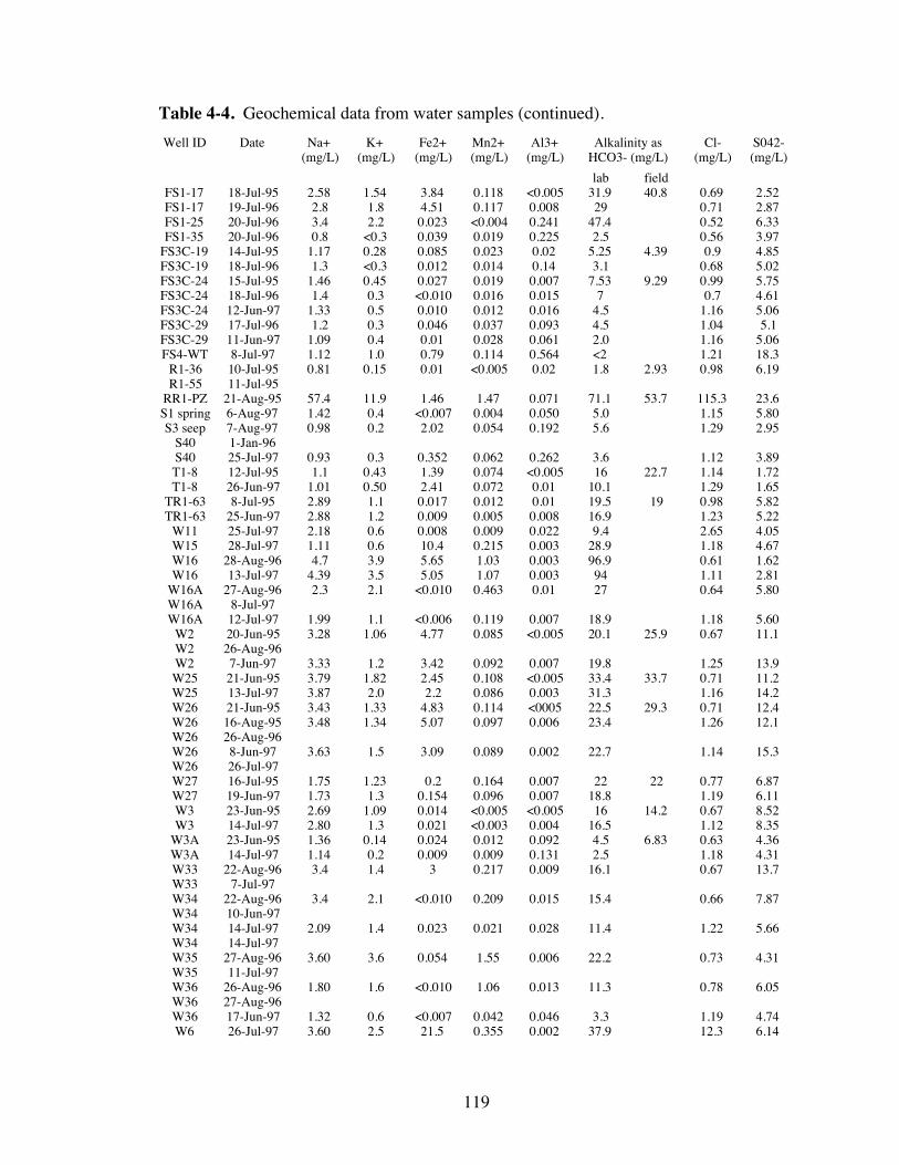
Table 4-4. Geochemical data from water samples (continued).

Well ID Date Na+(mg/L)

K+(mg/L)

Fe2+(mg/L)

Mn2+(mg/L)

Al3+(mg/L)

Alkalinity asHCO3- (mg/L)

Cl-(mg/L)

S042-(mg/L)

lab fieldFS1-17 18-Jul-95 2.58 1.54 3.84 0.118 <0.005 31.9 40.8 0.69 2.52FS1-17 19-Jul-96 2.8 1.8 4.51 0.117 0.008 29 0.71 2.87FS1-25 20-Jul-96 3.4 2.2 0.023 <0.004 0.241 47.4 0.52 6.33FS1-35 20-Jul-96 0.8 <0.3 0.039 0.019 0.225 2.5 0.56 3.97

FS3C-19 14-Jul-95 1.17 0.28 0.085 0.023 0.02 5.25 4.39 0.9 4.85FS3C-19 18-Jul-96 1.3 <0.3 0.012 0.014 0.14 3.1 0.68 5.02FS3C-24 15-Jul-95 1.46 0.45 0.027 0.019 0.007 7.53 9.29 0.99 5.75FS3C-24 18-Jul-96 1.4 0.3 <0.010 0.016 0.015 7 0.7 4.61FS3C-24 12-Jun-97 1.33 0.5 0.010 0.012 0.016 4.5 1.16 5.06FS3C-29 17-Jul-96 1.2 0.3 0.046 0.037 0.093 4.5 1.04 5.1FS3C-29 11-Jun-97 1.09 0.4 0.01 0.028 0.061 2.0 1.16 5.06FS4-WT 8-Jul-97 1.12 1.0 0.79 0.114 0.564 <2 1.21 18.3

R1-36 10-Jul-95 0.81 0.15 0.01 <0.005 0.02 1.8 2.93 0.98 6.19R1-55 11-Jul-95

RR1-PZ 21-Aug-95 57.4 11.9 1.46 1.47 0.071 71.1 53.7 115.3 23.6S1 spring 6-Aug-97 1.42 0.4 <0.007 0.004 0.050 5.0 1.15 5.80S3 seep 7-Aug-97 0.98 0.2 2.02 0.054 0.192 5.6 1.29 2.95

S40 1-Jan-96S40 25-Jul-97 0.93 0.3 0.352 0.062 0.262 3.6 1.12 3.89T1-8 12-Jul-95 1.1 0.43 1.39 0.074 <0.005 16 22.7 1.14 1.72T1-8 26-Jun-97 1.01 0.50 2.41 0.072 0.01 10.1 1.29 1.65

TR1-63 8-Jul-95 2.89 1.1 0.017 0.012 0.01 19.5 19 0.98 5.82TR1-63 25-Jun-97 2.88 1.2 0.009 0.005 0.008 16.9 1.23 5.22

W11 25-Jul-97 2.18 0.6 0.008 0.009 0.022 9.4 2.65 4.05W15 28-Jul-97 1.11 0.6 10.4 0.215 0.003 28.9 1.18 4.67W16 28-Aug-96 4.7 3.9 5.65 1.03 0.003 96.9 0.61 1.62W16 13-Jul-97 4.39 3.5 5.05 1.07 0.003 94 1.11 2.81

W16A 27-Aug-96 2.3 2.1 <0.010 0.463 0.01 27 0.64 5.80W16A 8-Jul-97W16A 12-Jul-97 1.99 1.1 <0.006 0.119 0.007 18.9 1.18 5.60

W2 20-Jun-95 3.28 1.06 4.77 0.085 <0.005 20.1 25.9 0.67 11.1W2 26-Aug-96W2 7-Jun-97 3.33 1.2 3.42 0.092 0.007 19.8 1.25 13.9W25 21-Jun-95 3.79 1.82 2.45 0.108 <0.005 33.4 33.7 0.71 11.2W25 13-Jul-97 3.87 2.0 2.2 0.086 0.003 31.3 1.16 14.2W26 21-Jun-95 3.43 1.33 4.83 0.114 <0005 22.5 29.3 0.71 12.4W26 16-Aug-95 3.48 1.34 5.07 0.097 0.006 23.4 1.26 12.1W26 26-Aug-96W26 8-Jun-97 3.63 1.5 3.09 0.089 0.002 22.7 1.14 15.3W26 26-Jul-97W27 16-Jul-95 1.75 1.23 0.2 0.164 0.007 22 22 0.77 6.87W27 19-Jun-97 1.73 1.3 0.154 0.096 0.007 18.8 1.19 6.11W3 23-Jun-95 2.69 1.09 0.014 <0.005 <0.005 16 14.2 0.67 8.52W3 14-Jul-97 2.80 1.3 0.021 <0.003 0.004 16.5 1.12 8.35

W3A 23-Jun-95 1.36 0.14 0.024 0.012 0.092 4.5 6.83 0.63 4.36W3A 14-Jul-97 1.14 0.2 0.009 0.009 0.131 2.5 1.18 4.31W33 22-Aug-96 3.4 1.4 3 0.217 0.009 16.1 0.67 13.7W33 7-Jul-97W34 22-Aug-96 3.4 2.1 <0.010 0.209 0.015 15.4 0.66 7.87W34 10-Jun-97W34 14-Jul-97 2.09 1.4 0.023 0.021 0.028 11.4 1.22 5.66W34 14-Jul-97W35 27-Aug-96 3.60 3.6 0.054 1.55 0.006 22.2 0.73 4.31W35 11-Jul-97W36 26-Aug-96 1.80 1.6 <0.010 1.06 0.013 11.3 0.78 6.05W36 27-Aug-96W36 17-Jun-97 1.32 0.6 <0.007 0.042 0.046 3.3 1.19 4.74W6 26-Jul-97 3.60 2.5 21.5 0.355 0.002 37.9 12.3 6.14

120

Table 4-4. Geochemical data from water samples (continued).

Well ID Date NO3-(mg/L)

F-(mg/L)

Br-(mg/L)

TotalCations

meq

TotalAnions

(meq) labalk.

TotalAnions(meq)

field alk.

ChargeBal %lab alk.

ChargeBal %

field alk.

Si(mg/L)

FS1-17 18-Jul-95 0.14 0 0.671 0.597 0.743 11.63 -10.21FS1-17 19-Jul-96 0.06 0.04 <0.01 0.71 0.56 23.7 5.01FS1-25 20-Jul-96 0.13 0.06 0.02 1.89 0.93 68.11 6.64FS1-35 20-Jul-96 0.01 0.06 <0.01 0.16 0.14 14.08 3.02

FS3C-19 14-Jul-95 0.15 0 0.164 0.215 0.201 -26.99 -20.3FS3C-19 18-Jul-96 0.02 0.06 <0.01 0.19 0.18 7.14 3.24FS3C-24 15-Jul-95 0.08 0 0.232 0.272 0.301 -15.85 -25.81FS3C-24 18-Jul-96 0.03 0.04 <0.01 0.23 0.23 -0.41 4.12FS3C-24 12-Jun-97 0.13 <0.05 <0.02 0.2 0.214 -6.68 3.49FS3C-29 17-Jul-96 0.1 0.08 <0.01 0.21 0.22 -2.61 3.38FS3C-29 11-Jun-97 0.16 0.01 <0.02 0.166 0.174 -4.27 2.77FS4-WT 8-Jul-97 <0.10 0.06 <0.02 0.401 0.418 -4.11 4.33

R1-36 10-Jul-95 0.13 0 0.161 0.188 0.207 -15.33 -24.62R1-55 11-Jul-95

RR1-PZ 21-Aug-95 10.5 0 4.846 5.078 4.793 -4.68 1.1S1 spring 6-Aug-97 0.62 0.05 <0.02 0.258 0.248 4.09 4.01S3 seep 7-Aug-97 <0.10 0.05 <0.02 0.192 0.192 0.00 2.02

S40 1-Jan-96S40 25-Jul-97 <0.10 0.06 <0.02 0.156 0.174 -10.8 3.94T1-8 12-Jul-95 0.18 0 0.206 0.333 0.443 -47.3 -73.2T1-8 26-Jun-97 <0.10 <0.05 <0.02 0.239 0.236 1.1 2.68

TR1-63 8-Jul-95 0.37 0 0.45 0.474 0.466 -5.31 -3.57TR1-63 25-Jun-97 0.30 0.06 <0.02 0.433 0.428 1.16 8.43

W11 25-Jul-97 0.89 0.04 <0.02 0.338 0.33 2.45 4.23W15 28-Jul-97 <0.10 <0.05 <0.02 0.607 0.604 0.43 2.49W16 28-Aug-96 <0.01 0.49 <0.01 1.82 1.66 8.99 11.4W16 13-Jul-97 0.73 0.49 <0.02 1.734 1.668 3.87 11.9

W16A 27-Aug-96 0.09 0.1 <0.01 0.54 0.59 -9.04 7.7W16A 8-Jul-97W16A 12-Jul-97 0.25 0.12 <0.02 0.421 0.470 -11.1 6.0

W2 20-Jun-95 0.08 0 0.699 0.581 0.676 18.5 3.38W2 26-Aug-96W2 7-Jun-97 <0.10 0.11 <0.02 0.675 0.655 3.03 9.2W25 21-Jun-95 0.08 0 0.813 0.802 0.807 1.39 0.77W25 13-Jul-97 <0.10 0.22 <0.02 0.845 0.853 -1.01 8.66W26 21-Jun-95 0.08 0 0.769 0.648 0.76 17.04 1.22W26 16-Aug-95 0.02 0 0.798 0.671 17.29W26 26-Aug-96W26 8-Jun-97 <0.10 0.15 <0.02 0.745 0.730 2.00 9.5W26 26-Jul-97W27 16-Jul-95 0.17 0 0.497 0.528 0.528 -6.04 -6.04W27 19-Jun-97 <0.10 0.05 <0.02 0.471 0.472 -0.10 5.9W3 23-Jun-95 0.09 0 0.411 0.46 0.43 -11.17 -4.55W3 14-Jul-97 <0.10 0.09 <0.02 0.466 0.481 -2.99 8.7

W3A 23-Jun-95 0.05 0 0.162 0.183 0.221 -12.53 -31.23W3A 14-Jul-97 <0.10 0.08 <0.02 0.166 0.168 -1.19 3.41W33 22-Aug-96 <0.01 0.13 <0.01 0.66 0.57 13.61 9.8W33 7-Jul-97W34 22-Aug-96 0.02 0.08 0.01 0.45 0.44 2.94 7.34W34 10-Jun-97 0.25 0.05 <0.02 0.335 0.346 -3.06 6.52W34 14-Jul-97W34 14-Jul-97W35 27-Aug-96 <0.01 0.07 <0.01 0.46 0.48 -3.07 7.2W35 11-Jul-97W36 26-Aug-96 0.02 0.05 <0.01 0.33 0.34 -2.23 5.03W36 27-Aug-96W36 17-Jun-97 <0.10 0.05 <0.02 0.183 0.192 -4.37 3.99W6 26-Jul-97 1.79 0.05 0.02 1.141 1.128 1.2 8.85

121

Table 4-4. Geochemical data from water samples (continued).

Well ID Date B3+(mg/L)

Ba2+(mg/L)

Li+(mg/L)

Cu(mg/L)

Zn(mg/L)

traceNO2

tracePO4

traceoxalate

Deuterium(per mil

VSMOW)FS1-17 18-Jul-95 -66.14FS1-17 19-Jul-96 <0.005 0.005 0.014 0.016 0.275 y y -68.4FS1-25 20-Jul-96 <0.005 0.009 0.016 0.011 0.005 y y -66.3FS1-35 20-Jul-96 <0.005 0.011 0.002 0.121 0.018 -61.1

FS3C-19 14-Jul-95 -66.6FS3C-19 18-Jul-96 <0.005 0.006 0.002 0.277 0.095 -62.4FS3C-24 15-Jul-95 -67.02FS3C-24 18-Jul-96 <0.005 0.003 0.002 0.303 0.178 -63.9FS3C-24 12-Jun-97 <0.005 0.002 0.002 0.039 0.067 -69.83FS3C-29 17-Jul-96 <0.005 0.004 0.004 0.841 0.14 y -66.5FS3C-29 11-Jun-97 <0.005 0.003 0.003 0.017 0.044 -70.58FS4-WT 8-Jul-97 <0.005 0.016 0.004 0.018 0.040 -71.03

R1-36 10-Jul-95 -67.21R1-55 11-Jul-95 -67.37

RR1-PZ 21-Aug-95 -59.88S1 spring 6-Aug-97 <0.005 0.004 0.002 0.004 0.023 -64.67S3 seep 7-Aug-97 <0.005 0.007 0.001 0.004 0.058 -68.16

S40 1-Jan-96S40 25-Jul-97 <0.005 0.006 0.002 0.010 0.021 -61.48T1-8 12-Jul-95 -81.32T1-8 26-Jun-97 <0.005 0.002 <0.001 0.007 0.176 -61.82

TR1-63 8-Jul-95 -67.26TR1-63 25-Jun-97 <0.005 0.002 0.008 0.173 0.021 -65.41

W11 25-Jul-97 <0.005 0.004 <0.001 0.024 0.057 -65.67W15 28-Jul-97 <0.005 0.006 0.002 0.003 1.70 -64.25W16 28-Aug-96 <0.005 0.006 0.029 0.002 0.159 -64W16 13-Jul-97 <0.005 0.007 0.027 0.002 0.189 -65.64

W16A 27-Aug-96 <0.005 0.003 0.013 0.006 0.028 -65.6W16A 8-Jul-97W16A 12-Jul-97 <0.005 0.002 0.009 0.003 0.010 -63.55

W2 20-Jun-95 -49.51W2 26-Aug-96W2 7-Jun-97 <0.005 0.004 0.008 0.004 0.046 -63.68W25 21-Jun-95 -69.07W25 13-Jul-97 <0.005 0.004 0.024 0.019 0.010 -66.89W26 21-Jun-95 -65.01W26 16-Aug-95W26 26-Aug-96W26 8-Jun-97 <0.005 0.004 0.012 0.004 0.041 -64.56W26 26-Jul-97W27 16-Jul-95 -68.97W27 19-Jun-97 <0.005 0.004 0.004 0.002 0.008 -66.75W3 23-Jun-95 -63.31W3 14-Jul-97 <0.005 0.001 0.008 0.124 0.009 -66.13

W3A 23-Jun-95 -65.83W3A 14-Jul-97 <0.005 0.003 0.001 0.007 0.028 -69.15W33 22-Aug-96 <0.005 0.003 0.01 0.007 0.023 -63.2W33 7-Jul-97W34 22-Aug-96 <0.005 0.002 0.009 0.016 0.032 y -66.4W34 10-Jun-97 <0.005 0.001 0.006 0.004 0.046 -66.41W34 14-Jul-97W34 14-Jul-97W35 27-Aug-96 <0.005 0.004 0.003 0.005 0.027 -64.4W35 11-Jul-97W36 26-Aug-96 <0.005 0.004 0.002 0.005 0.016W36 27-Aug-96W36 17-Jun-97 <0.005 0.003 0.002 0.004 0.011 -66.00W6 26-Jul-97 <0.005 0.004 0.024 0.003 0.366 -69.20

122

Table 4-4. Geochemical data from water samples (continued).

Well ID Date Oxygen-18 (per milVSMOW)

TritiumTU

Tritium 1

sig TU

C-13 (permil

VPDB)

CFC-11a CFC-11b CFC-11c CFC-12a CFC-12b

FS1-17 18-Jul-95 -10.14 13.1 0.4 -22.81 9025.8 5455.4 4206.8 392.8 366.9FS1-17 19-Jul-96 -10.37 12 0.4 -21.9 6214 8481.4 6223.2 85.8 389.2FS1-25 20-Jul-96 -10.11 13.2 0.4 -15.7 9403.3 88830.6 9083.3 427.1 393.6FS1-35 20-Jul-96 -9.42 10.3 0.4 -24.5 ERR ERR ERR 1089.6 1355.5

FS3C-19 14-Jul-95 -10.08 12.5 0.4 -16.4 1110.7 1096.3 1060.5 408.7 417.3FS3C-19 18-Jul-96 -9.71 9.9 0.3 -24.7 812.9 786.6 860.4 389.3 382.7FS3C-24 15-Jul-95 -10.12 12.3 0.4 -24.05 1116.5 1135.2 1092.7 439.2 461.1FS3C-24 18-Jul-96 -9.97 11.8 0.4 -20.1 939.8 953.1 976.1 396.5 402.7FS3C-24 12-Jun-97 -10.58 8.80 0.4 -21.50FS3C-29 17-Jul-96 -9.84 10.3 0.4 -20.5 952.3 680 931.7 382.2 281.7FS3C-29 11-Jun-97 -10.87 9.70 0.4 -17.57FS4-WT 8-Jul-97 -10.66 11.80 0.5 -17.16

R1-36 10-Jul-95 -10.14 12.8 0.4 -22.57 922.1 922.9 892.5 422.1 421R1-55 11-Jul-95 -9.95 11.1 0.4 -13.52 ERR 342.1 ERR 609.5 441.6

RR1-PZ 21-Aug-95 -9.01 13.7 0.4 -20.76 4133.8 4255.1 4421.6 411.5 376.4S1 spring 6-Aug-97 -9.99 8.50 0.4 -19.19S3 seep 7-Aug-97 -10.37 10.10 0.4 -28.14

S40 1-Jan-96 12.1 0.4S40 25-Jul-97 -9.36 12.60 0.5 -27.10T1-8 12-Jul-95 -12.02 9.4 0.3 -16.35 781.8 727.8 736.1 407.2 374.3T1-8 26-Jun-97 -9.31 8.70 0.4

TR1-63 8-Jul-95 -10.06 12.2 0.4 -23.42 5770.7 5561 5181.4 347.9 361.4TR1-63 25-Jun-97 -9.92 11.20 0.5

W11 25-Jul-97 -9.73 10.30 0.5 -22.31W15 28-Jul-97 -9.76 11.00 0.5 -21.51W16 28-Aug-96 -9.91 3.4 0.18 -10.6 59.8 89.4 94.3 31.7 42.8W16 13-Jul-97 -9.88 3.40 0.3 -10.21

W16A 27-Aug-96 -9.91 11.8 0.4 -18.1 569.3 600 664 303.8 430.4W16A 8-Jul-97W16A 12-Jul-97 -9.85 9.90 0.5 -16.94

W2 20-Jun-95 -5.62 16.6 0.5 -21.48 8.9 11.2 240 250W2 26-Aug-96W2 7-Jun-97 -9.71 14.80 0.6 -20.96W25 21-Jun-95 -10.4 -20.54 137.2 165.7 161.3 166.8 178W25 13-Jul-97 -10.25 24.40 0.8 -20.25W26 21-Jun-95 -9.97 22.4 0.7 6.4 3.9 4.6 172.7 193.3W26 16-Aug-95W26 26-Aug-96W26 8-Jun-97 -9.87 17.80 0.6 -20.66W26 26-Jul-97W27 16-Jul-95 -10.66 12.1 0.4 -23.65 784.5 783.8 390.6W27 19-Jun-97 -9.96 9.20 0.4W3 23-Jun-95 -9.79 14.4 0.4 503.6 507.5 507.9 333.6 342.4W3 14-Jul-97 -9.85 12.00 0.5 -22.54

W3A 23-Jun-95 -10.07 12.5 0.4 -12.67 932.4 947.8 921 423.4 430.7W3A 14-Jul-97 -10.60 9.60 0.4 -19.24W33 22-Aug-96 -9.74 12.8 0.4 -20.6 389 58.9 514.1 254.8 247.9W33 7-Jul-97 -9.76 14.20 0.6 -20.83W34 22-Aug-96 -9.98 12 0.4W34 10-Jun-97 -10.22 10.90 0.5 -24.78W34 14-Jul-97W34 14-Jul-97W35 27-Aug-96 -9.79 10.6 0.4 -20.7W35 11-Jul-97 -10.15 10.10 0.5W36 26-Aug-96 10.1 0.3 -23.3 753.8 737.8 734.4 385.6 387.9W36 27-Aug-96W36 17-Jun-97 -9.98 9.50 0.4 -18.92W6 26-Jul-97 -10.45 10.70 0.5 -21.20

123

Table 4-4. Geochemical data from water samples (continued).

Well ID Date CFC-12c CFC-113a

CFC-113b

CFC-113c

CFC-11avg

CFC-12avg

CFC-113avg

oldageCFC-11

oldageCFC-12

FS1-17 18-Jul-95 359.3 ERR 63.6 75.7 contam. 6FS1-17 19-Jul-96 386 48.8 149.4 106.2 contam. 28FS1-25 20-Jul-96 372.3 224.1 162 119.9 contam. 7.5FS1-35 20-Jul-96 1128.7 ERR ERR ERR ERR contam.

FS3C-19 14-Jul-95 419.9 118 131.3 129.5 1089.17 415.3 126.267 contam. 0FS3C-19 18-Jul-96 377.8 163.6 148.4 153.2 11 7FS3C-24 15-Jul-95 432.9 242.9 214.5 205 1114.8 444.4 contam. 0FS3C-24 18-Jul-96 386.2 154.2 161.1 145.8 7 6.5FS3C-24 12-Jun-97FS3C-29 17-Jul-96 381.8 182.8 130.1 169.1 14 13.5FS3C-29 11-Jun-97FS4-WT 8-Jul-97

R1-36 10-Jul-95 421.1 175.5 173.4 181.7 912.5 421.4 6 0R1-55 11-Jul-95 234.6 ERR ERR ERR 22 15

RR1-PZ 21-Aug-95 415.6 163.4 191 159 contam. 4S1 spring 6-Aug-97S3 seep 7-Aug-97

S40 1-Jan-96S40 25-Jul-97T1-8 12-Jul-95 377.5 102.3 105.6 110.3 10.5 4.5T1-8 26-Jun-97

TR1-63 8-Jul-95 351.6 80.9 87.5 82.3 contam. 7TR1-63 25-Jun-97

W11 25-Jul-97W15 28-Jul-97W16 28-Aug-96 40.9 57.5 26.7 29.6 34 35.5W16 13-Jul-97

W16A 27-Aug-96 313.1 102.9 107.3 98 18 12W16A 8-Jul-97W16A 12-Jul-97

W2 20-Jun-95 0 0 10.05 245 0 41.5 14.5W2 26-Aug-96W2 7-Jun-97W25 21-Jun-95 171 11.3 15.3 15.1 154.733 172 13.9 28 20.5W25 13-Jul-97W26 21-Jun-95 180.1 0 0 0 4.96667 182 0 44 20.5W26 16-Aug-95W26 26-Aug-96W26 8-Jun-97W26 26-Jul-97W27 16-Jul-95 398.8 102.5 97.7 784.15 395 100.1 9 2.5W27 19-Jun-97W3 23-Jun-95 340.2 59 62.3 62.7 506.333 338.667 61.3333 18 8W3 14-Jul-97

W3A 23-Jun-95 424.1 104.4 105.4 92.6 933.733 426 100.533 1.5 0W3A 14-Jul-97W33 22-Aug-96 234.9 15.7 5.4 13.9 34 17W33 7-Jul-97W34 22-Aug-96W34 10-Jun-97W34 14-Jul-97W34 14-Jul-97W35 27-Aug-96W35 11-Jul-97W36 26-Aug-96 430.6 115.3 190.7 230.1 12 6.5W36 27-Aug-96W36 17-Jun-97W6 26-Jul-97

124

Table 4-4. Geochemical data from water samples (continued).

Well ID Date oldageCFC-113

CH4(mg/L)

CH4 b CO2(mg/L)

CO2 b N2(mg/L)

N2 b O2(mg/L)

O2 b

FS1-17 18-Jul-95 10.5FS1-17 19-Jul-96 14FS1-25 20-Jul-96 6FS1-35 20-Jul-96 ERR

FS3C-19 14-Jul-95 3.5FS3C-19 18-Jul-96 contam.FS3C-24 15-Jul-95 contam.FS3C-24 18-Jul-96 contam.FS3C-24 12-Jun-97 0.0000 18.735 17.270 8.655FS3C-29 17-Jul-96 4.5FS3C-29 11-Jun-97FS4-WT 8-Jul-97 0.0003 0.0003 60.638 75.126 17.776 20.749 5.447 5.352

R1-36 10-Jul-95 contam. 0 6.8 28.04 11.7R1-55 11-Jul-95 ERR 0.486 0.1 21.86 0.2

RR1-PZ 21-Aug-95 contam.S1 spring 6-Aug-97S3 seep 7-Aug-97

S40 1-Jan-96S40 25-Jul-97 0.0174 0.0350 37.805 37.957 16.420 18.105 0.662 0.740T1-8 12-Jul-95 6 0.013 14.6 19.71 4.7T1-8 26-Jun-97 0.0574 0.0488 16.640 17.325 18.701 18.709 4.100 4.229

TR1-63 8-Jul-95 8.5 0 11.6 20.55 8.6TR1-63 25-Jun-97 0.0000 10.322 21.804 10.576

W11 25-Jul-97 0.0000 0.0000 36.689 36.163 21.534 19.509 8.186 7.426W15 28-Jul-97 0.0139 0.0130 25.765 25.443 18.507 18.434 0.678 0.700W16 28-Aug-96 18.5 0.5624 0.5663 3.648 2.775 21.55 20.963 0.248 0.115W16 13-Jul-97 0.1891 0.2847 12.883 12.274 21.248 21.214 0.020 0.080

W16A 27-Aug-96 8.5W16A 8-Jul-97 0.0005 0.0005 16.731 16.974 19.708 19.416 5.511 5.432W16A 12-Jul-97 0.0000 0.0009 15.093 15.050 18.768 18.670 6.833 6.839

W2 20-Jun-95 >30.5W2 26-Aug-96 0.0011 19.911 19.507 0.405W2 7-Jun-97 0.0000 9.298 16.818 0.048W25 21-Jun-95 25.5W25 13-Jul-97 0.0000 0.0000 7.425 7.450 21.482 21.485 0.061 0.033W26 21-Jun-95 >30.5W26 16-Aug-95W26 26-Aug-96 0 7.083 20.759 0.018W26 8-Jun-97 0.0000 13.576 18.865 0.402W26 26-Jul-97W27 16-Jul-95 6.5W27 19-Jun-97 0.0024 19.698 18.503 3.831W3 23-Jun-95 11W3 14-Jul-97 0.0006 0.0007 17.304 17.317 21.014 20.751 2.682 2.762

W3A 23-Jun-95 6W3A 14-Jul-97 0.0000 0.0000 36.813 37.075 20.366 21.253 3.660 3.961W33 22-Aug-96 30.5 0 6.81 20.32 0.376W33 7-Jul-97 0.0004 0.0005 7.968 7.735 20.100 20.291 0.027 0.065W34 22-Aug-96 0.0014 7.14 20.15 3.618W34 10-Jun-97 0.0000 6.285 17.481 8.253W34 14-Jul-97 0.0000 0.0001 8.498 8.795 19.384 19.368 7.757 7.239W34 14-Jul-97 0.0000 8.773 19.526 7.499W35 27-Aug-96 0.0051 14.571 34.163 5.947W35 11-Jul-97 0.0052 0.0060 21.778 21.049 21.397 21.502 5.693 6.086W36 26-Aug-96 6.5 0.0025 19.308 19.106 4.005W36 27-Aug-96 0.0029 18.707 20.775 4.298W36 17-Jun-97 0.0000 19.284 17.639 9.285W6 26-Jul-97 0.7135 0.9744 12.952 10.973 19.729 19.838 0.000 0.015

125

Table 4-4. Geochemical data from water samples (continued).

Well ID Date Ar(mg/L)

Ar b Lab notes

FS1-17 18-Jul-95FS1-17 19-Jul-96 FE dropping out in FUFS1-25 20-Jul-96FS1-35 20-Jul-96

FS3C-19 14-Jul-95FS3C-19 18-Jul-96FS3C-24 15-Jul-95FS3C-24 18-Jul-96FS3C-24 12-Jun-97 0.7073FS3C-29 17-Jul-96FS3C-29 11-Jun-97FS4-WT 8-Jul-97 0.6725 0.7257 downhole °C

R1-36 10-Jul-95 0.8659R1-55 11-Jul-95 0.7812

RR1-PZ 21-Aug-95S1 spring 6-Aug-97 spring °CS3 seep 7-Aug-97 downhole °C

S40 1-Jan-96S40 25-Jul-97 0.6096 0.6330T1-8 12-Jul-95 0.7279T1-8 26-Jun-97 0.7030 0.7036

TR1-63 8-Jul-95 0.7328TR1-63 25-Jun-97 0.7849

W11 25-Jul-97 0.7629 0.7427W15 28-Jul-97 0.6767 0.6618W16 28-Aug-96 0.7721 0.7543 Fe dropping out in FUW16 13-Jul-97 0.7715 0.7708

W16A 27-Aug-96W16A 8-Jul-97 0.7393 0.7356W16A 12-Jul-97 0.7077 0.7089

W2 20-Jun-95W2 26-Aug-96 0.7361W2 7-Jun-97 0.6620W25 21-Jun-95W25 13-Jul-97 0.7800 0.7760W26 21-Jun-95W26 16-Aug-95W26 26-Aug-96 0.7496W26 8-Jun-97 0.7125W26 26-Jul-97W27 16-Jul-95W27 19-Jun-97 0.7054W3 23-Jun-95W3 14-Jul-97 0.7661 0.7632

W3A 23-Jun-95W3A 14-Jul-97 0.7507 0.7738W33 22-Aug-96 0.7262 Fe dropping out in FUW33 7-Jul-97 0.7570 0.7618W34 22-Aug-96 0.7368W34 10-Jun-97 0.6774W34 14-Jul-97 0.7219 0.7236W34 14-Jul-97 0.7175W35 27-Aug-96 0.9135 diss.gas leaked?W35 11-Jul-97 0.7708 0.7636 downhole °CW36 26-Aug-96 0.7124 4 CFC analysesW36 27-Aug-96 0.7475W36 17-Jun-97 0.7012W6 26-Jul-97 0.6980 0.7064

126

300 260R1

TR2

FS2

FS1

FS3

W27

W25W3,3A

W34

W33

W2

W15

W16,16A

W36

W35

W26

S3

0

0

100 meters

300 feet

71°42'

LANDSURFACE ELEVATION-IN METERS (VARIABLEINTERVAL)-

ROAD-

PIEZOMETER-

WELL CLUSTER-

SEEP

W2

FS2

S3

43°56'40"

43°56'50

71°41'50"71°42'10"

HQ

FS3C

S40

300 260

240

deepshallow

DO range changed-between samples

DO 2 - 5 mg/L

DO £ 1 mg/L

DO ³ 6 mg/L

Not-Sampled

W Stream

Figure 4-13 Spatial distribution of dissolved oxygen concentrations in water samples

from piezometers at the Mirror Lake site, Grafton County, New Hampshire.

127

Major ion concentrations characterize the overall water quality of the shallow

ground-water in the Mirror Lake watershed (Table 4-4). The general water type is

calcium-bicarbonate-sulfate in piezometers (fig. 4-14). Outliers include: RR1-PZ located

below the Mirror Lake watershed between Route 3 and the Pemigewasset River in an

agricultural area; W6 located adjacent to Mirror Lake Road, also contains nitrate; W11

behind an experimental sand plot that has been fertilized, also contains nitrate; FS1-25

100

80 60 40 20 0 100

80

60

40

20

SOD

IUM

+ POTA

SSIUM

MAG

NESI

UM

100806040200

SULFA

TEBIC

ARBO

NATE

100

80

60

40

20

0

CHLO

RID

E +

SULF

ATE

100

80

60

40

20

0

100

80

60

40

20

0

CALC

IUM

+ MA

GNE

SIUM

0

CALCIUM

100

80 60 40 20 0 100

80

60

40

20

SOD

IUM

+ POTASSIU

M

100

80

60

40

20

0

MAG

NES

IUM

100806040200

100

80

60

40

20

0

CHLORIDE

SULFATEBI

CAR

BON

ATE

100

80

60

40

20

0

CH

LOR

IDE

+ SU

LFAT

E

100

80

60

40

20

0

100

80

60

40

20

0

CALC

IUM

+ MAG

NESIU

M0

RR1-PZW6

W11

FS4-WT

R1-36

W16

W35W6

RR1-PZ

W35

W6

RR1-PZFS1-25

W16

FS1-25

W16

FS4-WT

Figure 4-14 Piper plot of major ions in samples from piezometers.

128

apparently contaminated from well construction materials; W16, a steel well screened

several meters below the water table; and R1-36, a high-yielding well with low alkalinity

and high sulfate. New piezometers for this study include FS4-WT, installed high in the

watershed near the basin divide, that has low alkalinity and high sulfate, and that also

contains high CO2; and W35 that contains high potassium.

Nitrogen and argon dissolved gas concentrations (Table 4-4) indicate that little

excess air is present near the water table, and that the recharge temperature is between 5

and 10°C (fig. 4-15). Concentrations of dissolved nitrogen gas and argon in ground water

are used to infer the recharge temperature and excess air amounts (Heaton and Vogel,

1981). These quantities are used in turn to determine equilibrium air concentrations from

measured water concentrations to date ground water by the CFC method (Busenberg and

Plummer, 1992). In contrast to samples from bedrock wells at Mirror Lake (Busenberg

and Plummer, 1996), nitrogen and argon concentrations fall approximately along the line

corresponding to equilibration with the atmosphere. This suggests that the elevated argon

and nitrogen in bedrock waters is not due to entrapped or excess air, but is caused by

some other in situ production.

Methane is observed in several samples from water-table piezometers.

Measurable methane and lack of DO are consistent with methanogenic biodegradation

conditions near the water table.

129

0.4

0.6

0.8

1

1.2

1.4

10 15 20 25 30 35 40 45 50

AR

GO

N (

mg/

L)

NITROGEN (mg/L)

0

Excess Air (cc/L)

10

20

RechargeTemperature

30 °C

20 °C

10 °C

0 °C

BEDROCK

DRIFT

Figure 4-15 Concentrations of dissolved argon and nitrogen in water samples from

piezometers (solid symbols) and packer-isolated zones of bedrock wells (open

symbols) at the Mirror Lake site, Grafton County, New Hampshire. The superposed

grid indicates the concentrations of argon and nitrogen in water that is in equilibrium

with the atmosphere as a function of temperature, and that contains varying volumes

of entrapped dissolved air.

130

4.3.4 Chlorofluorocarbon Concentrations

CFC concentrations in water samples from shallow piezometers range from zero

to levels greater than those in equilibrium with the modern (1995-1997) atmosphere

(Table 4-4). Many samples do contain CFC concentrations near modern atmospheric-

equilibrium levels, which are about 950, 450, and 150 pg/kg for CFC-11, -12, and -113,

respectively (at 7 °C). This observation supports use of CFC concentrations to date

saturated-zone ground water.

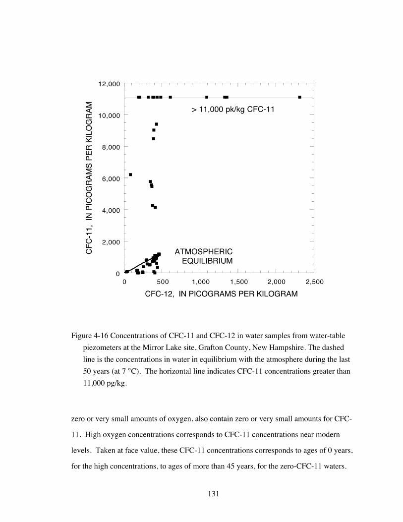
Many samples contain CFC concentrations higher than those in equilibrium with

the atmosphere (fig. 4-16). Following Busenberg and Plummer (1992), these samples are

designated Òcontaminated.Ó In some cases, contamination of samples was so high that

the analytical procedures used to concentrate the normal low levels resulted in analytical

responses beyond the instrumentation limits (ÒERRÓ results in Table 4-4).

However, many samples contain CFC concentrations significantly less than those

in equilibrium with the modern atmosphere. A preliminary review of the data indicated

that CFC concentrations were highly correlated with dissolved oxygen (DO)

concentrations. For this reason, the CFC data are plotted here against DO (fig. 4-17).

CFC-12 concentrations range from about 170 pg/kg to about 2,300 pg/kg (Table

4-4). For uncontaminated samples, CFC-12 concentrations are correlated with DO (fig.

4-17). Samples containing zero or very small amounts of oxygen, have CFC-12

concentrations about 1/3 of the concentration of water in equilibrium with modern air.

High oxygen concentrations correspond to CFC-12 concentrations near modern levels.

Concentrations of CFC-11 range from zero to 88,000 pg/kg (Table 4-4). Some

samples were so highly contaminated with CFC-11 that quantification of the

concentrations was not analytically possible (Table 4-4). For uncontaminated samples,

CFC-11 concentrations are strongly correlated with DO (fig. 4-18). Samples containing

131

0

2,000

4,000

6,000

8,000

10,000

12,000

0 500 1,000 1,500 2,000 2,500

CF

C-1

1, I

N P

ICO

GR

AM

S P

ER

KIL

OG

RA

M

CFC-12, IN PICOGRAMS PER KILOGRAM

ATMOSPHERICEQUILIBRIUM

> 11,000 pk/kg CFC-11

Figure 4-16 Concentrations of CFC-11 and CFC-12 in water samples from water-table

piezometers at the Mirror Lake site, Grafton County, New Hampshire. The dashed

line is the concentrations in water in equilibrium with the atmosphere during the last

50 years (at 7 °C). The horizontal line indicates CFC-11 concentrations greater than

11,000 pg/kg.

zero or very small amounts of oxygen, also contain zero or very small amounts for CFC-

11. High oxygen concentrations corresponds to CFC-11 concentrations near modern

levels. Taken at face value, these CFC-11 concentrations corresponds to ages of 0 years,

for the high concentrations, to ages of more than 45 years, for the zero-CFC-11 waters.

132

150

200

250

300

350

400

450

-2 0 2 4 6 8 10 12

CF

C-1

2 C

ON

CE

NT

RA

TIO

N,

IN P

IKO

GR

AM

S P

ER

KIL

OG

RA

M

DISSOLVED OXYGEN, IN MILLIGRAMS PER LITER

APPARENT AGE0 YEARS

20 YEARS

Figure 4-17 Concentrations of CFC-12 and dissolved oxygen in water samples from

piezometers at the Mirror Lake site, Grafton County, New Hampshire. The

horizontal lines correspond to CFC-12 concentrations in water equilibrated with the

atmosphere at the time of sampling (0 years) and 20 years before sampling.

133

0

200

400

600

800

1000

1200

-2 0 2 4 6 8 10 12

CF

C-1

1 C

ON

CE

NT

RA

TIO

N,

IN P

IKO

GR

AM

S P

ER

KIL

OG

RA

M

DISSOLVED OXYGEN, IN MILLIGRAMS PER LITER

APPARENT AGE0 YEARS

20 YEARS

Figure 4-18 Concentrations of CFC-11 and dissolved oxygen in water samples from

piezometers at the Mirror Lake site, Grafton County, New Hampshire. The

horizontal lines correspond to CFC-11 concentrations in water equilibrated with the

atmosphere at the time of sampling (0 years) and 20 years before sampling.

Concentrations of CFC-113 range from zero to 240 pg/kg (Table 4-4). Some

samples were so highly contaminated with CFC-113 that quantification of the

concentrations was not analytically possible (Table 4-4). For uncontaminated samples,

CFC-113 concentrations are strongly correlated with DO (fig. 4-19). Samples containing

134

0

50

100

150

200

-2 0 2 4 6 8 10 12

CF

C-1

13 C

ON

CE

NT

RA

TIO

N,

IN P

IKO

GR

AM

S P

ER

KIL

OG

RA

M

DISSOLVED OXYGEN, IN MILLIGRAMS PER LITER

APPARENT AGE0 YEARS

20 YEARS

Figure 4-19 Concentrations of CFC-113 and dissolved oxygen in water samples from

piezometers at the Mirror Lake site, Grafton County, New Hampshire. The horizontal

lines correspond to CFC-113 concentrations in water equilibrated with the

atmosphere at the time of sampling (0 years) and 20 years before sampling.

zero or very small amounts of oxygen, also contain zero or very small amounts for CFC-

113. High oxygen concentrations corresponds to CFC-113 concentrations near modern

levels. The scatter in CFC-113 concentrations in high-DO samples is larger than the

scatter for either CFC-12 or CFC-11.

135

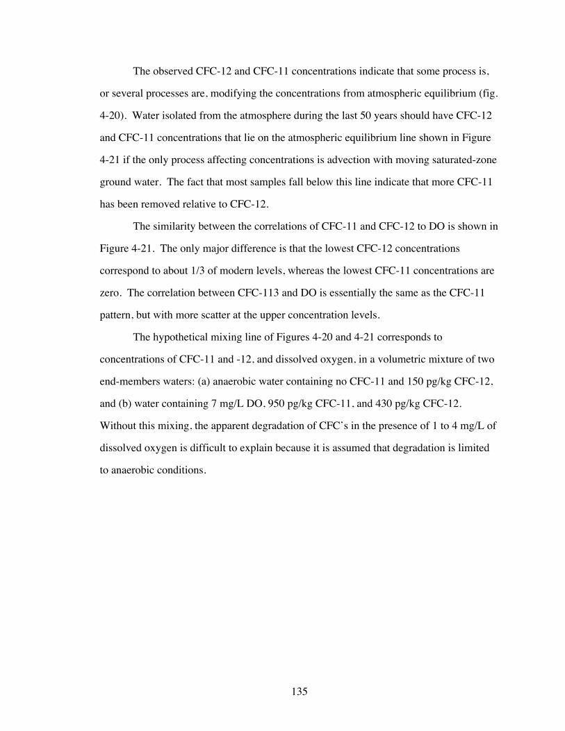
The observed CFC-12 and CFC-11 concentrations indicate that some process is,

or several processes are, modifying the concentrations from atmospheric equilibrium (fig.

4-20). Water isolated from the atmosphere during the last 50 years should have CFC-12

and CFC-11 concentrations that lie on the atmospheric equilibrium line shown in Figure

4-21 if the only process affecting concentrations is advection with moving saturated-zone

ground water. The fact that most samples fall below this line indicate that more CFC-11

has been removed relative to CFC-12.

The similarity between the correlations of CFC-11 and CFC-12 to DO is shown in

Figure 4-21. The only major difference is that the lowest CFC-12 concentrations

correspond to about 1/3 of modern levels, whereas the lowest CFC-11 concentrations are

zero. The correlation between CFC-113 and DO is essentially the same as the CFC-11

pattern, but with more scatter at the upper concentration levels.

The hypothetical mixing line of Figures 4-20 and 4-21 corresponds to

concentrations of CFC-11 and -12, and dissolved oxygen, in a volumetric mixture of two

end-members waters: (a) anaerobic water containing no CFC-11 and 150 pg/kg CFC-12,

and (b) water containing 7 mg/L DO, 950 pg/kg CFC-11, and 430 pg/kg CFC-12.

Without this mixing, the apparent degradation of CFCÕs in the presence of 1 to 4 mg/L of

dissolved oxygen is difficult to explain because it is assumed that degradation is limited

to anaerobic conditions.

136

0

200

400

600

800

1000

1200

0 100 200 300 400 500

CF

C-1

1, I

N P

IKO

GR

AM

S P

ER

KIL

OG

RA

M

CFC-12, IN PIKOGRAMS PER KILOGRAM

ATMOSPHERICEQUILIBRIUM

Figure 4-20 Concentrations of CFC-11 and CFC-12 in water samples from water-table

piezometers at the Mirror Lake site, Grafton County, New Hampshire. The dashed

line is the concentrations in water in equilibrium with the atmosphere during the last

50 years (at 7 °C). The solid line is a suggested mixing line.

137

0

200

400

600

800

1000

1200

150

200

250

300

350

400

450

500

-2 0 2 4 6 8 10 12

CFC-11

CFC-12

CF

C-1

1 C

ON

CE

NT

RA

TIO

N,

IN P

IKO

GR

AM

S P

ER

KIL

OG

RA

M

CF

C-1

2 C

ON

CE

NT

RA

TIO

N,

IN P

IKO

GR

AM

S P

ER

KIL

OG

RA

M

DISSOLVED OXYGEN, IN MILLIGRAMS PER LITER

APPARENT AGE0 YEARS

LINEAR MIXTURE

Figure 4-21 Concentrations of CFC-11, CFC-12, and dissolved oxygen in water samples

from water-table piezometers at the Mirror Lake site, Grafton County, New

Hampshire. The horizontal line corresponds to CFC-11 and CFC-12 concentrations

in water equilibrated with the atmosphere at the time of sampling. The solid line is a

suggested mixing line.

The relation between CFC-11 and tritium in samples from water-table piezometer

is shown in Figure 4-22. Assuming an equilibration temperature of 7 °C, the CFC-11

concentration in water recharged in 1963 would be about 62 pg/kg. The concentration of

tritium in waters recharged in 1963, accounting for subsequent radioactive decay until

138

0

5

10

15

20

25

0 200 400 600 800 1000 1200

TR

ITIU

M,

IN T

RIT

IUM

UN

ITS

CFC-11, IN PICOGRAMS PER KILOGRAM

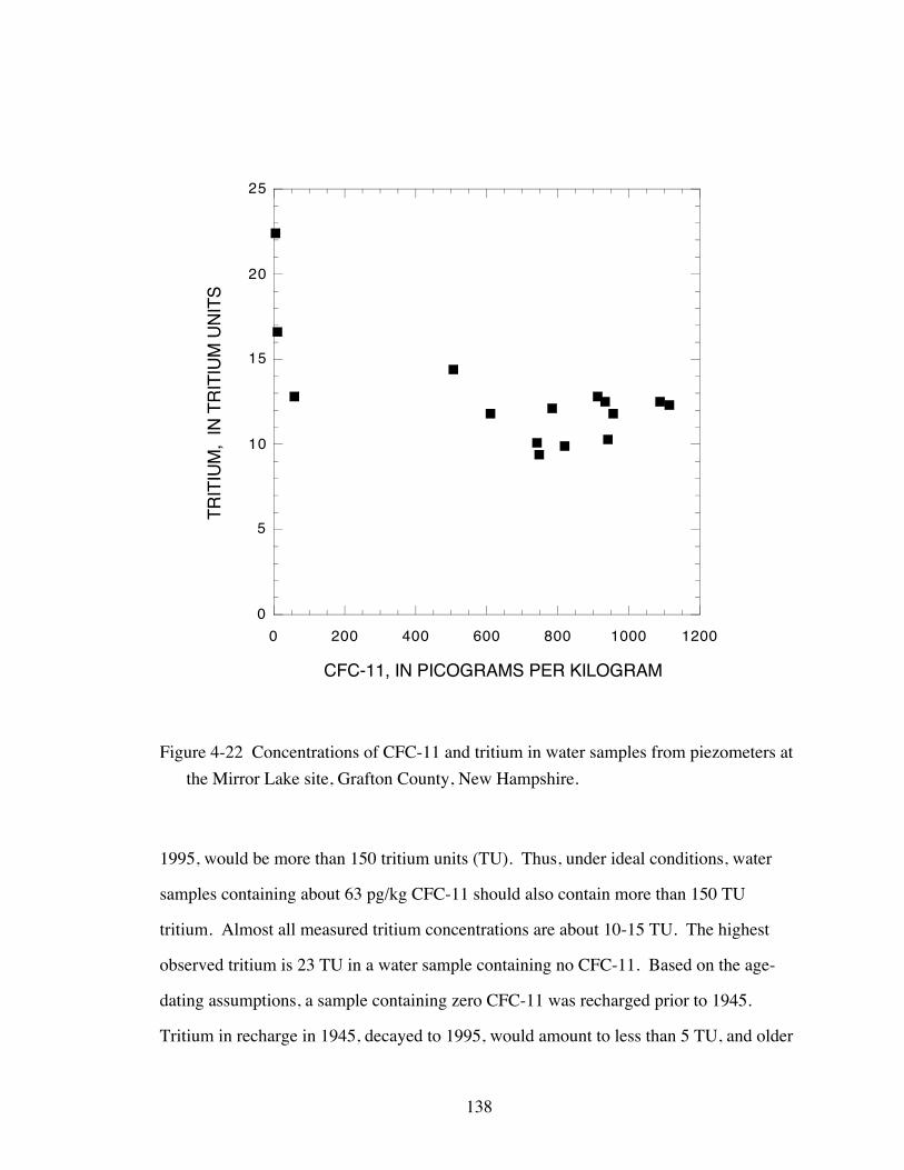
Figure 4-22 Concentrations of CFC-11 and tritium in water samples from piezometers at

the Mirror Lake site, Grafton County, New Hampshire.

1995, would be more than 150 tritium units (TU). Thus, under ideal conditions, water

samples containing about 63 pg/kg CFC-11 should also contain more than 150 TU

tritium. Almost all measured tritium concentrations are about 10-15 TU. The highest

observed tritium is 23 TU in a water sample containing no CFC-11. Based on the age-

dating assumptions, a sample containing zero CFC-11 was recharged prior to 1945.

Tritium in recharge in 1945, decayed to 1995, would amount to less than 5 TU, and older

139

waters would contain even less tritium. All of these tritium concentrations are

significantly below bomb-peak levels dating from the late 50Õs and early 60Õs.

Busenberg and Plummer (1996) estimate that peak tritium levels in precipitation in New

Hampshire from the early 1960Õs decayed to 1992 would amount to about 300 TU, over

an order of magnitude higher than the values observed here. The observed tritium and

CFC concentrations suggest that these water samples represent modern recharge, but that

CFC concentrations have been reduced by degradation.

Concentrations of CFCÕs in soil gas exhibit much less variability than liquid

concentrations (Table 4-5). All CFC-12 soil gas concentrations are close to 100 percent

of modern atmospheric levels (fig. 4-23). The average CFC-12 soil gas concentration at

each sampling location ranges from 0.97 to 1.06 times modern air concentrations. CFC-

12 concentrations in local air are close to the global average, with individual

measurements ranging from 0.97 to 1.01 times the global average.

CFC-11 concentrations vary somewhat more than CFC-12 concentrations and are

reduced compared to modern air. The average CFC-11 soil gas concentration at each

sampling location range from 0.82 to 1.01 times modern air concentrations. CFC-11 soil

gas concentrations are low near well W33 (fig. 4-24), where zero CFC-11 is measured in

shallow water-table piezometers, and where the water table is anaerobic (fig. 4-13).

CFC-113 concentrations vary somewhat more than either CFC-12 or CFC-11

concentrations, and several locations exhibit reduced concentrations compared to modern

air. The average CFC-113 soil gas concentration at each sampling location ranged from

0.83 to 1.08 times modern air concentrations. CFC-113 soil gas concentrations are low

near well W33, where zero CFC-113 is measured in shallow water-table piezometers, and

where the water table is anaerobic (fig. 4-13).

CFC concentrations in soil gas show essentially no correlation with depth.

However, in a few cases, a systematic pattern in time occurs. In these cases, the winter

soil gas CFC-11 and CFC-113 concentrations are a lower fraction of modern air than the

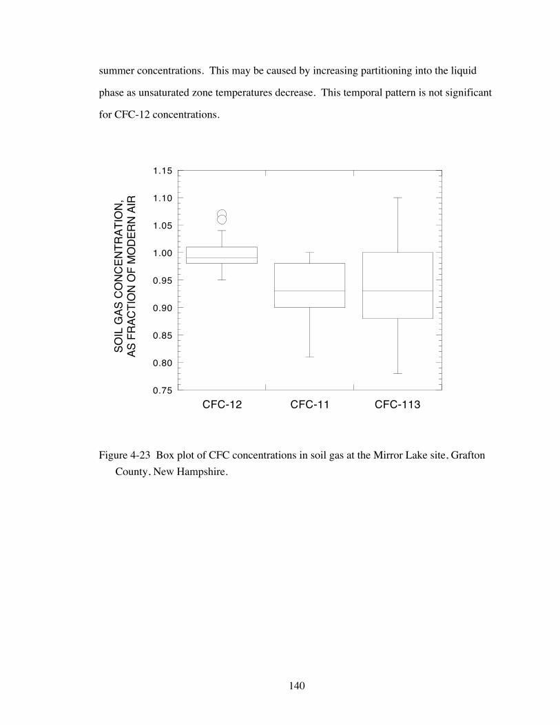
140

summer concentrations. This may be caused by increasing partitioning into the liquid

phase as unsaturated zone temperatures decrease. This temporal pattern is not significant

for CFC-12 concentrations.

0.75

0.80

0.85

0.90

0.95

1.00

1.05

1.10

1.15

CFC-12 CFC-11 CFC-113

SO

IL G

AS

CO

NC

EN

TR

AT

ION

,A

S F

RA

CT

ION

OF

MO

DE

RN

AIR

Figure 4-23 Box plot of CFC concentrations in soil gas at the Mirror Lake site, Grafton

County, New Hampshire.

141

Table 4-5. Concentrations of CFCÕs in soil gas.

Screen Sample Sample Sequence Concentration in gas (pptv) Fraction of Air ConcentrationID depth (cm) date time Lab Field CFC-12 CFC-11 CFC-113 CFC-12 CFC-11 CFC-113 Notes

W33-red 140 30-Jan-97 1536 1 525.4 226.5 70.0 0.98 0.83 0.8330-Jan-97 1546 2 523.3 224.9 69.2 0.97 0.82 0.82 lab time 1548

avg 0.97 0.82 0.83W33-white 200 30-Jan-97 1512 1 525.2 232.3 71.6 0.98 0.85 0.85

30-Jan-97 1518 2 535.0 223.1 69.5 0.99 0.81 0.8330-Jan-97 1525 3 521.9 233.5 71.0 0.97 0.85 0.84

avg 0.98 0.84 0.84W33-blue 240 30-Jan-97 1440 1 529.2 237.1 73.0 0.98 0.87 0.87

30-Jan-97 1455 3 526.0 233.9 71.8 0.98 0.85 0.85avg 0.98 0.86 0.86

W2-blue 100FS2-R25 0 29-Jan-97 1600 R-25 530.1 276.6 91.1 0.99 1.01 1.08

29-Jan-97 1600 R-25 534.4 275.1 91.1 0.99 1.00 1.08avg 0.99 1.01 1.08

FS2-air 0 17-Jul-96 910 3 530.9 255.4 79.8 0.99 0.93 0.95 lab date 7/7/9617-Jul-96 913 3 526.1 252.8 78.2 0.98 0.92 0.93

avg 0.98 0.93 0.94FS2-red 65 17-Jul-96 849 1 535.9 258.2 82.3 1.00 0.94 0.98 low flow rate

17-Jul-96 853 2 530.4 267.5 83.8 0.99 0.98 1.0017-Jul-96 856 3 537.8 273.1 87.5 1.00 1.00 1.0529-Jan-97 1205 1 545.0 253.9 80.1 1.01 0.93 0.95

avg 1.00 0.96 1.00FS2-blue 180 17-Jul-96 749 1 1 536.5 261.8 82.0 1.00 0.96 0.98 purged 1 min,

50 sec ea.sample

17-Jul-96 753 2 2 528.9 269.9 91.8 0.98 0.99 1.1017-Jul-96 756 3 3 510.5 257.8 83.1 0.95 0.94 0.99 lab time was

1651?29-Jan-97 1237 1 1 537.4 252.7 80.3 1.00 0.92 0.9529-Jan-97 1242 2 2 542.7 246.5 75.5 1.01 0.90 0.9029-Jan-97 1247 3 3 535.7 250.8 77.5 1.00 0.92 0.92

avg 0.99 0.94 0.97

142

Table 4-5. Concentrations of CFCÕs in soil gas (continued).

Screen Sample Sample Sequence Concentration in gas (pptv) Fraction of Air ConcentrationID depth (cm) date time Lab Field CFC-12 CFC-11 CFC-113 CFC-12 CFC-11 CFC-113 Notes

W34 180W25-red 95W25-white 190W25-blue 300FS1-red 90 29-Aug-96 1715 522.5 271.7 86.6 0.97 0.99 1.04

29-Aug-96 1722 529.6 270.9 88.5 0.99 0.99 1.06avg 0.98 0.99 1.05

FS1-blue 180FS3-air 0 31-Jan-97 1034 528.5 260.9 86.0 0.98 0.95 1.02FS3 200 31-Jan-97 1012 1 1 538.1 249.4 74.6 1.00 0.91 0.89

31-Jan-97 1019 2 2 536.3 242.0 65.9 1.00 0.88 0.7831-Jan-97 1024 3 3 527.8 247.0 73.8 0.98 0.90 0.88

avg 0.99 0.90 0.85FS3-red 130FS3-blue 215 30-Jan-97 1603 1 1 577.8 268.5 75.4 1.07 0.98 0.90 lab fs3c

30-Jan-97 1608 2 2 568.1 267.2 77.0 1.06 0.98 0.9130-Jan-97 1613 3 3 561.6 273.9 78.6 1.04 1.00 0.93

avg 1.06 0.99 0.91FS3T-red 60 16-Jul-96 1630 2 1 541.6 266.6 83.0 1.01 0.97 0.99 lab fs3

16-Jul-96 1635 1 3 532.9 265.0 79.8 0.99 0.97 0.9530-Jan-97 1637 1 1 531.6 252.8 77.2 0.99 0.92 0.92 labeled fs3c-a30-Jan-97 1645 2 2 534.7 243.9 73.4 0.99 0.89 0.8730-Jan-97 1651 3 3 532.2 253.2 77.9 0.99 0.92 0.92

avg 0.99 0.94 0.93FS3T-white 120 16-Jul-96 1559 1 1 535.1 271.8 86.8 1.00 0.99 1.04

16-Jul-96 1610 3 536.5 269.7 84.2 1.00 0.98 1.0131-Jan-97 917 1 1 523.3 246.4 77.0 0.97 0.90 0.9131-Jan-97 922 2 2 544.1 241.6 73.1 1.01 0.88 0.8731-Jan-97 927 3 3 524.9 247.4 79.7 0.98 0.90 0.95

avg 0.99 0.93 0.95

143

Table 4-5. Concentrations of CFCÕs in soil gas (continued).

Screen Sample Sample Sequence Concentration in gas (pptv) Fraction of Air ConcentrationID depth (cm) date time Lab Field CFC-12 CFC-11 CFC-113 CFC-12 CFC-11 CFC-113 Notes

FS3T-blue 180 16-Jul-96 1548 3 534.5 266.4 89.2 0.99 0.97 1.0716-Jul-96 1534 1 1 530.7 270.2 88.7 0.99 0.99 1.06 lab time 1630?31-Jan-97 936 1 1 539.4 262.0 77.2 1.00 0.96 0.9231-Jan-97 941 2 2 547.6 253.7 74.8 1.02 0.93 0.8931-Jan-97 946 3 3 554.0 257.0 76.0 1.03 0.94 0.90 lab fs3c

avg 1.01 0.96 0.97W36-R6 0 31-Jan-97 1400 R-6 529.8 265.6 82.3 0.99 0.97 0.98

31-Jan-97 1400 R-6 530.6 264.4 82.3 0.99 0.97 0.98avg 0.99 0.97 0.98

W36-air 0 29-Aug-96 1453 519.6 254.4 79.8 0.97 0.93 0.95W36-red 60 29-Aug-96 1504 1 1 516.3 251.5 77.8 0.96 0.92 0.93

29-Aug-96 1511 3 3 520.9 250.6 79.0 0.97 0.91 0.94 lab time 1610?31-Jan-97 1538 1 1 525.8 242.6 73.7 0.98 0.89 0.88

avg 0.97 0.91 0.92W36-white 150 29-Aug-96 1539 1 1 520.8 260.6 83.2 0.97 0.95 0.99

29-Aug-96 1546 3 3 534.2 259.7 80.5 0.99 0.95 0.9631-Jan-97 1559 1 1 546.4 253.7 74.4 1.02 0.93 0.8831-Jan-97 1605 2 2 549.7 249.7 71.7 1.02 0.91 0.8531-Jan-97 1610 3 3 542.5 251.6 71.9 1.01 0.92 0.85

avg 1.00 0.93 0.91W36-blue 260 29-Aug-96 1600 3 2 551.8 270.1 83.8 1.03 0.99 1.00

29-Aug-96 1604 1 3 531.6 271.7 88.5 0.99 0.99 1.0631-Jan-97 1623 1 1 546.7 268.5 86.4 1.02 0.98 1.0331-Jan-97 1634 3 3 547.4 270.4 85.8 1.02 0.99 1.02

avg 1.01 0.99 1.03FS4-R12 0 30-Jan-97 945 R-12 541.9 278.7 95.1 1.01 1.02 1.13

30-Jan-97 945 R-12 530.4 280.8 96.8 0.99 1.03 1.15avg 1.00 1.02 1.14

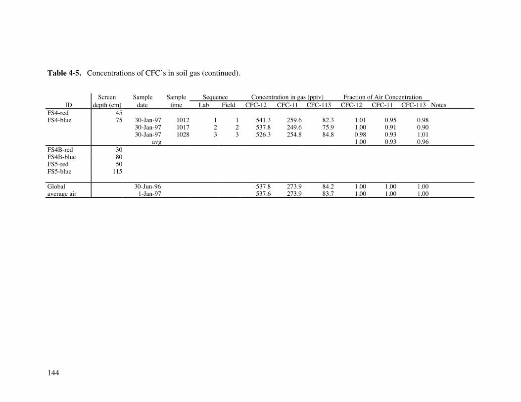
144

Table 4-5. Concentrations of CFCÕs in soil gas (continued).

Screen Sample Sample Sequence Concentration in gas (pptv) Fraction of Air ConcentrationID depth (cm) date time Lab Field CFC-12 CFC-11 CFC-113 CFC-12 CFC-11 CFC-113 Notes

FS4-red 45FS4-blue 75 30-Jan-97 1012 1 1 541.3 259.6 82.3 1.01 0.95 0.98

30-Jan-97 1017 2 2 537.8 249.6 75.9 1.00 0.91 0.9030-Jan-97 1028 3 3 526.3 254.8 84.8 0.98 0.93 1.01

avg 1.00 0.93 0.96FS4B-red 30FS4B-blue 80FS5-red 50FS5-blue 115

Global 30-Jun-96 537.8 273.9 84.2 1.00 1.00 1.00average air 1-Jan-97 537.6 273.9 83.7 1.00 1.00 1.00

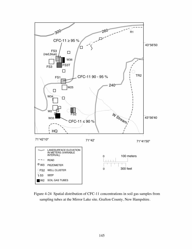
145

300 R1

TR2

FS2

FS1

FS3

W25

W34

W33

W2

W36

0

0

100 meters

300 feet

71°42'

LANDSURFACE ELEVATION-IN METERS (VARIABLEINTERVAL)-

ROAD-

PIEZOMETER-

WELL CLUSTER-

SEEP-

SOIL GAS TUBES

W3

FS2

S3

43°56'40"

43°56'50

71°41'50"71°42'10"

HQ

300

240

FS3(red,blue)

FS3T

W2

260

W Stream CFC-11 ≤ 90 %

CFC-11 90 - 95 %

CFC-11 ≥ 95 %

Figure 4-24 Spatial distribution of CFC-11 concentrations in soil gas samples from

sampling tubes at the Mirror Lake site, Grafton County, New Hampshire.

146

4.4 Discussion

The goals of this field study involve characterization of the concentrations of

CFCÕs in water recharging the saturated zone. Where dissolved oxygen concentrations

are relatively high (greater than 5 mg/L), CFC concentrations at the water table appear to

be approximately in equilibrium with the modern atmosphere. However, even in these

well-oxygenated samples, there is significant variability in CFC concentrations. The

observed range of concentrations in aerobic water-table samples corresponds to

uncertainty in ground-water ages determined from CFC-12, CFC-11, and CFC-113

concentrations on the order of ± 4, 7, and 8 years, respectively. This variability in

concentrations at the water table presumably impacts the uncertainty in ages associated

with water samples from deeper in the saturated zone at the Mirror Lake site. This

uncertainty is significantly larger than the analytical uncertainty in the laboratory (± 1 yr).

The hydraulic data collected during this study suggests that recharge is highest in

the early spring and fall, but recharge occurs throughout the year depending on the

intensity of precipitation. Significant recharge also occurs slowly throughout the winter,

and more rapidly in the winter during mid-winter snowmelt, when it occurs.

Soil temperatures are consistent with measured noble gas concentrations and

suggest that recharge temperatures at the water table range between 5 and 10 °C. The

average recharge temperature of 7 °C is probably a reasonable approximation for

estimating past atmospheric gas concentrations from water samples.

Samples from wells screened near the water table that contain low dissolved

oxygen also contain low CFCÕs, relative to atmospheric equilibrium. In the case of CFC-

11 and CFC-113, these compounds are completely absent from some anaerobic samples.

CFC-12 is not reduced as much, with concentrations in anaerobic samples as low as 1/3

of modern levels. Ground water in the saturated zone that was anaerobic shortly after

recharge near the water table is likely to have low CFC concentrations. These low CFC

147

concentrations would yield apparent ages for deeper saturated-zone samples much larger

than the actual time since recharge.

CFC concentrations are also significantly reduced in samples that have dissolved

oxygen concentrations ranging from 1-4 mg/L. This pattern is not consistent with

degradation of CFCÕs only under anaerobic conditions because these DO levels are not

low enough to be considered anaerobic. However, this pattern of intermediate CFC

concentrations in samples having intermediate DO is consistent with a linear mixing

model.

The general pattern of the correlation between CFCÕs and DO suggests a linear

mixing model, although there is scatter in the measurements. This mixing model

assumes that samples are linear mixtures of two end-members: (a) aerobic water having

about 6 mg/L DO and CFC concentrations in equilibrium with the modern atmosphere;

and (b) anaerobic water having no oxygen, no CFC-11 or CFC-113, and CFC-12

concentrations about 1/3 of modern atmospheric-equilibrium levels. That a water sample

pumped from a well with a 0.6 to 0.9 m long screen represents a mixture is not surprising.

Numerous investigators have reported small-scale water-quality variation in ground water

(e.g. Cozarelli et al., 1996). Such small-scale variability is supported by limited diffusion

in saturated ground water, and by large variations in permeability. Other evidence of

mixing of samples is the presence of iron (II) and methane in oxygenated samples. With

this mixing model, the lower concentrations in low-DO waters are explained not as

degradation under low-DO conditions, but as degradation under anaerobic conditions,

occurring in only a fraction of the total sample volume.

Anaerobic degradation of CFC-11 and CFC-113 has been observed in the

laboratory (Lovely and Woodward, 1992) and the field (Cook et al., 1995; Plummer et

al., in press), although CFC-12 degradation has only recently been reported for ground

waters (Oster et al., 1996). These field results are consistent with the observations

reported herein in that CFC-12 is less degraded, but concentrations of CFC-12 are

148

apparently reduced to about 1/3 of modern levels; not complete degradation, but a

significant loss that would cause significant differences between apparent and actual

ground-water ages.

Independent evidence of anaerobic biodegradation is presented by hydrogen gas,

methane, and carbon dioxide concentrations measured in several piezometers (Table 4-3).

Hydrogen gas concentrations can identify the controlling redox processes in anaerobic

systems (Lovely and Goodwin, 1988). CFC-11 degradation has been observed in the

laboratory for sulfate-reduction and methanogenesis redox conditions (Lovely and

Woodward, 1992), both of which are indicated in sampled piezometers. Sulfate and iron

(II) are present in shallow ground water at Mirror Lake (fig. 4-25) to support sulfate-

reduction and iron-reduction reactions. There is limited laboratory evidence that iron (II)

may play a role in abiotic degradation of CFC-11 under anaerobic conditions (Lovely and

Woodward, 1992).

Overall, CFC-12 concentrations appear to be least affected by anaerobic

degradation or contamination. The use of CFC-12 for age-dating ground water is likely

to be more robust in the field, particularly for systems where anaerobic degradation

conditions may exist.

Given the variability in geochemical conditions observed in different water-table

piezometers, it is not possible to characterize the distribution of CFCÕs in recharge in the

Mirror Lake drainage basin on the basis of these 31 wells. These results suggest that in

areas where the shallow water table is anaerobic, CFCÕs in recharge will be significantly

reduced from modern equilibrium levels. Furthermore, concentrations may also be

reduced due to anaerobic degradation in micro-environments, even though the apparent

redox conditions in pumped samples are not anaerobic. However, it is likely that these

micro-environments will have relatively low permeability, and thus may play a less

important role in controlling recharge chemistry, which will be weighted toward the

conditions occurring in higher permeability zones.

149

0

1

2

3

4

5

0

2

4

6

8

10

12

14

0 200 400 600 800 1000 1200

Fe++

SO4

--

IRO

N (F

e-II)

, IN

MIL

LIG

RA

MS

PE

R L

ITE

R

SU

LFA

TE

, IN

MIL

LIG

RA

MS

PE

R L

ITE

R

CFC-11, IN PIKOGRAMS PER KILOGRAM

Figure 4-25 Iron (II) and sulfate as a function of CFC-11 concentrations.

A local flow system associated with streamloss and flow across a sandy terrace

exhibits strong anaerobic conditions. Shattuck (1991) identified an area in the Mirror

Lake drainage basin where the water table gradient is across the W stream (fig. 4-26). It

appears that in this area stream water may enter the subsurface and flow across the sandy

terrace to another branch of the W stream. Dissolved oxygen (DO) and total organic

carbon (TOC) concentrations in water-table piezometers along the apparent flow

direction (approximately) suggest that the provision of organic carbon to the aquifer by

150

0 20

meters

FS1

FS2

W33

W2

W26

S40W34

W3AW3

W25

S40

Figure 4-26 Water table elevations in the lower part of the W stream drainage basin

(Shattuck, 1991).

the stream may contribute to the anaerobic redox conditions (fig. 4-27). Organic carbon

may be carried into the aquifer from the bottom of the stream. Dissolved oxygen is

consumed by the biologic activity and is only slowly replenished by diffusion downward

through the unsaturated zone. This streamloss is not the only factor contributing to

anaerobic conditions because such low-DO environments are also present upgradient of

streams (for example, W25 in fig. 4-27).

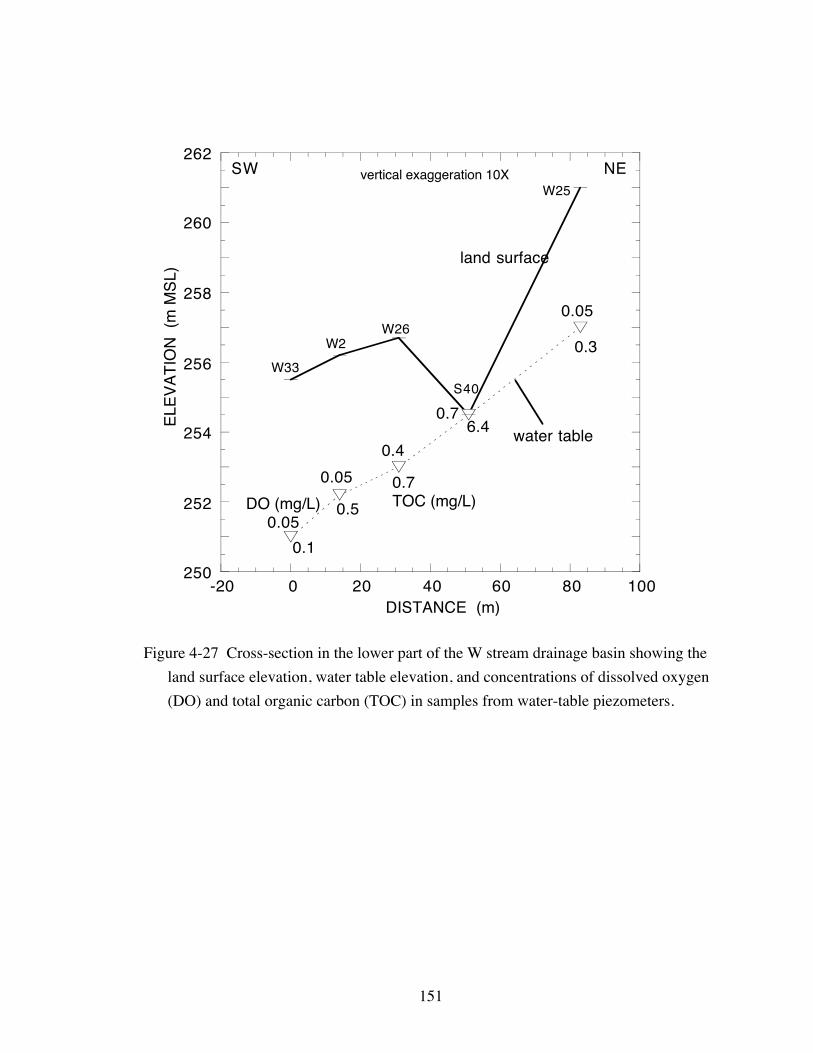
151

250

252

254

256

258

260

262

-20 0 20 40 60 80 100

ELE

VA

TIO

N (

m M

SL)

DISTANCE (m)

W33

W2W26

S40

W25

land surface

water table

vertical exaggeration 10XSW NE

DO (mg/L)0.05

0.05

0.4

0.7

0.05

0.1

0.5

0.7TOC (mg/L)

6.4

0.3

Figure 4-27 Cross-section in the lower part of the W stream drainage basin showing the

land surface elevation, water table elevation, and concentrations of dissolved oxygen

(DO) and total organic carbon (TOC) in samples from water-table piezometers.

152

4.5 Summary

The use of chlorofluorocarbons (CFC's) as age-dating tracers for ground water at

the Mirror Lake fractured-rock research site may be limited because concentrations of

CFC's in at least some areas are significantly reduced by anaerobic degradation. CFC

concentrations in water samples from high-conductivity fractures in schist and granite

bedrock indicate ages ranging from greater than 45 years to about 7 years, but the spatial

pattern of ages is complex and the youngest measured ages occur near the lake at the

bottom of the forested watershed. Equilibrium between CFC in the atmosphere and at the

water table is needed to date saturated-zone waters. However, samples from piezometers

screened just below the water table in the glacial drift indicate that CFC-11, CFC-12, and

CFC-113 are substantially degraded where dissolved oxygen (DO) concentrations are

low. Anaerobic (DO < 0.1 mg/L) conditions existing in a sandy terrace deposit may be

caused by biodegradation of organic carbon in infiltrating stream water. Samples from

this and other shallow anaerobic zones lack CFC-11 and CFC-113 and have CFC-12

concentrations that are as low as 1/3 of modern equilibrium concentrations. Furthermore,

several hypoxic (0.1 < DO < 3 mg/L) samples have significantly reduced CFC's. As

expected, samples with high DO collected at the water table generally contain CFC's near

atmospheric-equilibrium concentrations. Many samples plot on a mixing line for CFC's

and DO, suggesting that the water sampled can be a mixture of two end members: (1)

waters saturated with oxygen and containing CFC's in equilibrium with the modern

atmosphere, and (2) zero-DO waters containing no CFC-11 or CFC-113 and containing

about 1/3 of modern CFC-12. Several samples contain CFC-11 and CFC-113

concentrations higher than those from equilibration with peak atmospheric levels,

suggesting a non-atmospheric source. Possible sources of this contamination include

sampling equipment (Busenberg and Plummer, 1996) and well-construction materials,

including sand installed at well screens, grout used to seal the borehole annulus and PVC

153

adhesives. Evidence of active anaerobic biodegradation, which can degrade CFCÕs,

includes high methane and ample iron (Fe-II) and sulfate and generally low DO.

Hydrogen gas concentrations in anaerobic samples from water-table piezometers are

consistent with methanogenesis or sulfate-reduction as the terminal electron-accepting

process.

4.6 References

Bormann, F.H., and Likens, G.E., 1979, Patterns and Processes in a Forested Ecosystem: Springer-Verlag,New York, 253 p.

Bu, X., and Warner, M.J., 1995, Solubility of chlorofluorocarbon 113 in water and seawater: Deep SeaResearch, v. 42, no. 7, p. 11512-1161.

Bullister, J.L., and Lee, B.-S., 1995, Chlorofluorocarbon-11 removal in anoxic marine water: GeophysicalResearch Letters, v. 22, no. 14, p. 1893-1896.

Busenberg, E., and Plummer, L.N., 1992, Use of chlorofluorocarbons (CCl3F and CCl2F2) as hydrologictracers and age-dating tools: Example - The alluvium and terrace system of central Oklahoma: WaterResources Research, v. 28, p. 2257-2283.

Busenberg, E., and Plummer, L.N., 1993, Use of trichlorofluorocarbon-113 (CFC-113) as a hydrologictracer and age-dating tool of young ground water: GSA Abstracts with Programs, v. 25, no. 6, p. A-365.

Busenberg, E., and Plummer, L.N., 1996, Concentrations of chlorofluorocarbons and other gases in groundwater at Mirror Lake, New Hampshire: in Morganwalp, D.W., and Aronson, D.A., eds., U.S.Geological Survey Toxics Program Meeting, Colorado Springs, Colo., September 20-24, 1993: U.S.Geological Survey WRIR 94-4015.

Cook, P.G., Solomon, D.K., Plummer, L.N., Busenberg, E., and Schiff, S.L., 1995, Chlorofluorocarbons astracers of groundwater transport processes in a shallow, silty sand aquifer: Water Resources Research,v. 31, no. 3, p. 425-434.

Cozzarelli, I.M., Baedecker, M.J., Aiken, G., and Phinney, C.S., 1996, Small-scale chemicalheterogeneity's in a crude-oil-contaminated aquifer, Bemidji, Minnesota, in Morganwalp, D. W., andAronson, D.A., eds., U.S. Geological Survey Toxic Substances Hydrology Program - Proceedings ofthe Technical Meeting, Colorado Springs, Colorado, September 20-24, 1993: U.S. Geological SurveyWater-Resources Investigations Report 94-4015, p. 647-652.

Drenkard, S., Torgersen, T., Weppernig, R., Stute, M., Farley, K., and Schlosser, P., 1993, Helium isotopesand tritium-helium age dating: Mirror Lake, New Hampshire (abs.): GSA Abstracts with Programs, v.25, no. 6, p. A-364.

Dunkle, S.A., Plummer, L.N., Busenberg, E., Phillips, P.J., Denver, J.M., Hamilton, P.A., Michel, R.L., andCoplen, T.B., 1993, Chlorofluorocarbons (CCl3F and CCl2F2) as dating tools and hydrologic tracers inshallow ground water of the Delmarva Peninsula, Atlantic Coastal Plain, United States: WaterResources Research, v. 29, no. 12, p. 3837-3860.

Federer, C.A., 1973, Annual cycles of soil and water temperatures at Hubbard Brook: U.S. Forest ServiceResearch Note NE-167, 7 p.

154

Federer, C. A., Flynn, L. D., Martin, C. W., Hornbeck, J. W., and Pierce, R. S., 1990, Thirty years ofhydrometeorologic data at the Hubbard Brook Experimental Forest, New Hampshire: U.S.Department of Agriculture, Forest Service, Northeastern Forest Experiment Station, GeneralTechnical Report NE-141, 44 p.

Freeze, R.A., and J.A. Cherry, 1979, Groundwater, Prentice-Hall, Englewood Cliffs, New Jersey.

Goode, D.J., 1997, CFC transport to and degradation near a shallow water table, Mirror Lake area, GraftonCounty, New Hampshire: (abs.), p. S176 in 1997 Spring Meeting, supplement to Eos, 29 April 1997,American Geophysical Union, Washington DC.

Goode, D.J., Busenberg, Eurybiades, Plummer, L.N., Shapiro, A.M., and Vroblesky, D.A., 1997, CFCdegradation under anaerobic water table conditions in glacial drift at Mirror Lake New Hampshire:(abs.), Geological Society of America 1997 Annual Meeting, 20-23 October 1997, Salt Lake City,Utah, GSA Abstracts with Programs, vol. 29, no. 6, p. 77.

Harte, P.T., 1992, Regional ground-water flow in crystalline bedrock and interaction with glacial drift inthe New England uplands: M. S. Thesis, University of New Hampshire, Durham, 147 p.

Harte, P.T., 1997, Prelminary assessment of the lithologic and hydraulic properties of the glacial drift andshallow bedrock in the Mirror Lake area, Grafton County, New Hampshire: U.S. Geological SurveyOpen-File Report 96-654A, 56 p.

Harte, P.T. and Winter, T.C., 1995, Simulations of flow in fractured crystalline rock in a hypothetical NewEngland setting: Ground Water, v. 33, no. 3, p. 953-964.

Harte, P.T. and Winter, T.C., 1996, Factors affecting recharge to crystalline rock in the Mirror Lake area,Grafton County, New Hampshire: in Morganwalp, D.W., and Aronson, D.A., eds., U.S. GeologicalSurvey Toxics Program Meeting, Colorado Springs, Colo., September 20-24, 1993: U.S. GeologicalSurvey WRIR 94-4015.

Heaton, T.H.E., 1981, Dissolved gases: Some applications to groundwater research: Trans. Geol. Soc.South Africa, v. 84, p. 91-97.

Heaton, T.H.E., and Vogel, J.C., 1981, "Excess air" in groundwater: Journal of Hydrology, v. 41, p. 217-231.

Herkelrath, W.N., Hamburg, S.P., and Murphy, Fred, 1991, Real-time monitoring of soil moisture in aremote field area with time-domain reflectometry: Water Resources Research, v. 27, no. 5, p. 857-864.

Hsieh, P. A., Shapiro, A. M., Barton, C. C., Haeni, F. P., Johnson, C. D., Martin, C. W., Paillet, F. L.,Winter, T. C., and Wright, D. L., 1993, Methods of characterizing fluid movement and chemicaltransport in fractured rock: in Chaney, J. T., and Hepburn, C., (eds.) Field Trip Guidebook fornortheastern United States, Geological Society of America, annaul Meeting, October 25-28, 1993,Boston, Mass., v. 2, chap. R, p. R1-R23.

Hsieh, P.A., and Shapiro, A.M., 1996, Hydraulic characteristics of fractured bedrock underlying the FSEwell field at the Mirror Lake site, Grafton County, New Hampshire: in Morganwalp, D.W., andAronson, D.A., eds., U.S. Geological Survey Toxics Program Meeting, Colorado Springs, Colo.,September 20-24, 1993: U.S. Geological Survey WRIR 94-4015.

Khalil, M.A.K., and Rasmussen, R.A., 1989, The potential of soils as a sink of chlorofluorocarbons andother man-made chlorocarbons: Geophysical Research Letters, v. 16, no. 7, p. 679-682.

Khalil, M.A.K., and Rasmussen, R.A., 1993, The environmental history and probably future ofFluorocarbon 11: Journal of Geophysical Research, v. 98, no. D12, p. 23,091-23,106.

Likens, G. E., Bormann, F. H, 1995, Biogeochemistry of a Forested Ecosystem: Springer-Verlag, NewYork, 2nd ed., 159 p.

155

Likens, G. E. (ed.), 1985, An Ecosystem Approach to Aquatic Ecology, Mirror Lake and its Environment:Springer-Verlag, New York, 516 p.

Lovely, D.R., and Goodwin, S., 1988, Hydrogen concentrations as an indicator of the predominant terminalelectron-accepting reactions in aquatic sediments: Geochmica et Cosmochimica Acta, v. 52, p. 2993-3003.

Lovely, D.R., and Woodward, J.C., 1992, Consumption of Freon CFC-11 and CFC-12 by anaerobicsediments and soils: EST, v. 26, p. 925-929.

Mau, D.P., and Winter, T.C., 1997, Estimating ground-water recharge from streamflow hydrographs for asmall mountain watershed in a temperate humid climate, New Hampshire, USA: Ground Water, v. 35,no. 2, p. 291-304.

McConnell, J.B., Busenberg, E., and Plummer, L.N., 1994, Water-resources data for the Valdosta area,south-central Georgia, 1961-93: U.S. Geological Survey Open-file Report 94-350, 58 p.

Oster, H., C. Sonntag, and K.O. Munnich, 1996, Groundwater age dating with chlorofluorocarbons: WaterResources Research, v. 32, no. 10, p. 2989-3001.

Plummer, L. N., R.L. Michel, E.M. Thurman, and P.D. Glynn, 1993,. Environmental tracers for age datingyoung ground water, in Regional Ground-Water Quality , edited by W. M. Alley, pp. 255-294, VanNostrand Reinhold, New York.

Plummer, L.N., Busenberg, E., Drenkard, S., Schlosser, P., McConnell, J.B., Michel, R.L., Ekwurzel, B.,and Weppernig, R., (in press), Flow of river water into a karstic limestone aquifer--2. Dating theyoung fraction in groundwater mixtures in the upper Floridan Aquifer near Valdosta, Georgia, usingtritium/helium-3 and chlorofluorocarbons. (see data report: McConnell et al., 1994).

Reilly, T.E., L.N. Plummer, P.J. Phillips, and E. Busenberg, 1994, The use of simulation and multipleenvironmental tracers to quantify flow in a shallow aquifer: Water Resources Research, v. 30, no. 2,p. 421-433.

Russell, A.D., and Thompson, G.M., 1983, Mechanisms leading to enrichment of the atmosphericfluorocarbons CCl3F and CCl2F2 in groundwater: Water Resources Research, v. 19, no. 1, p. 57-60.

Semprini, L., Hopkins, G.D., Roberts, P.V., and McCarty, P.L., 1990, In-situ biotransformation of carbontetrachloride, 1,1,1-trichloroethane, Freon-11, and Freon-113 under anoxic conditions (abs.), in Eos,Trans. AGU, San Francisco, American Geophysical Union, p. 1324.

Shapiro, A.M., 1996, Using environmental tracers to estimate matrix diffusion in fractured rock overdistances of kilometers: Results from the Mirror Lake site, New Hampshire: Eos, Trans. AGU, v. 77,no. 17, p. S107.

Shapiro, A. M., and P. A. Hsieh, 1991, Research in fractured-rock hydrogeology: Characterizing fluidmovement and chemical transport in fractured rock at the Mirror Lake drainage basin, NewHampshire: p. 155-161 in Mallard, G.�E., and D. A. Aronson (eds.), U.S. Geol. Survey ToxicSubstances Hydrology Program--Proc. Technical Meeting, Monterey, California, March 11-15, 1991:U.S. Geol. Survey Water-Resources Invest. Rep. 91-4034.

Shapiro, A.M., Wood, W.W., Busenberg, E., Drenkard, S., Plummer, L.N., Torgersen, T., and Schlosser,P., 1996, Conceptual model for estimating regional fluid velocity in the bedrock of the Mirror Lakearea, Grafton County, New Hampshire, in Toxics Program Meeting, Colorado Springs, U.S.Geological Survey WRIR 94-4015.

Shattuck, P. C., 1991, Shallow water-table response to precipitation and evapotranspiration in an ephemeralstream valley, Woodstock, New Hampshire: unpublished M.S. Thesis, Hydrology Program,University of New Hampshire, Durham, 113 p.

156

Szabo, Z., D.E. Rice, L.N. Plummer, E. Busenberg, S. Drenkard, and P. Schlosser, 1996, Age dating ofshallow groundwater with chlorofluorocarbons, tritium/helium 3, and flow path analysis, southernNew Jersey coastal plain: Water Resources Research, v. 32, no. 4, p. 1023-1038.

Terauds, V.I., Contaldo, G., McCarthy, C.M., and Smith, G.B., 1993, Field and laboratory evidence for insitu biotransformation of isopropanol and Freon-11 (abs.): Ground Water, v. 31, no. 5, p. 850-851.

Thompson, G.M., and Hayes, J.M., 1979, Trichloromethane in groundwater - A possible tracer andindicator of groundwater age: Water Resources Research, v. 15, p. 546-554.

Thompson, G.M., Hayes, J.M., and Davis, S.N., 1974, Fluorocarbon tracers in hydrology: GeophysicalResearch Letters, v. 1, p. 177-180.

Tiedeman, C.R., Goode, D.J., and Hsieh, P.A., 1997, Numerical simulation of ground-water flow throughglacial deposits and crystalline bedrock in the Mirror Lake area, Grafton County, New Hampshire:U.S. Geological Survey Professional Paper 1572, 50 p.

U.S. Department of Agriculture Forest Service, 1991, The Hubbard Brook Ecosystem Study: Sitedescription and research activities: Northeastern Forest Experiment Station NE-INF0-96-91, 61 p.

Warner, M.J., and R.F. Weiss, 1985, Solubilities of chlorofluorocarbons 11 and 12 in water and seawater,Deep-Sea Research, v. 32, p. 1485-1497.

Weiss, R.F., 1970, The solubility of nitrogen, oxygen, and argon in water and seawater: Deep SeaResearch, v. 17, p. 721-735.

Wilson, Alicia, 1991, Distribution of hydraulic conductivity in the glacial drift at Hubbard BrookExperimental Forest, West Thornton, New Hampshire: unpublished Senior Honors Thesis, DartmouthCollege, Hanover, New Hampshrie, 56 p.

Winter, T. C., 1984, Geohydrologic setting of Mirror Lake, West Thornton, New Hampshire: U.S.Geological Survey Water-Resources Investigations Report 84-4266, 61 p.

Winter, T. C., 1985, Physiographic setting and geologic origin of Mirror Lake: in Likens, G. E., ed., Anecosystem approach to aquatic ecology: Mirror Lake and it Environment: Springer-Verlag, NewYork, p. 40-53.

Winter, T. C., Eaton, J. S., and Likens, G. E., 1989, Evaluation of inflow to Mirror Lake, New Hampshire:Water Resources Bulletin, vol. 25, no. 5, p. 991-1008.

Wood, W.W., Shapiro, A.M., and Councell, Terry, 1996, Observational experimental and inferred evidencefor solute diffusion in fractured granite aquifers: Examples from Mirror Lake Watershed, GraftonCounty, New Hampshire: in Morganwalp, D.W., and Aronson, D.A., eds., U.S. Geological SurveyToxics Program Meeting, Colorado Springs, Colo., September 20-24, 1993: U.S. Geological SurveyWRIR 94-4015.