1

Chapter-4- chemical equilibrium

توازن الكيميائيال -4-الفصل

This chapter develops the concept of chemical potential (الجهد الكيميائي) and shows how it is used to

account for the equilibrium composition of chemical reactions ( ميائية التوازن التركيبي للتفاعالت الكي ).

Main goals:

(1) Establishing the relation between the equilibrium constant (ثابتة التوازن) and the standard Gibbs

energy of reaction (طاقة جبس القياسية لتفاعل كيميائي).

(2) Establishing the quantitative effects of changes in the conditions ( تأثيرات الكمية بتغيير الشروط او ال

and description of the thermodynamic properties of reactions that take place in ;(الظروف

electrochemical cells (الخاليا الكهركيميائية), in which the reaction drives electrons through an external

circuit ( خارجيةالدارة الكهربائية ال ).

(3) Using thermodynamic arguments to derive the electric potential expression of electrochemical

cells and its relation to the composition of electrochemical cell. Two major topics developed in

this connection: (i) the definition and tabulation of standard potentials (الجهود القياسية); and (ii) The

second is the use of these standard potentials to determine the equilibrium constants and other

thermodynamic properties of chemical reactions.

(4) Using thermodynamics to predict the equilibrium composition under any reaction conditions

and understand the underlying molecular processes.

(5) Applying ideas related to chemical equilibria in electrochemistry field.

Spontaneous chemical reactions التفاعالت الكيميائية التلقائية

The direction of spontaneous change (اتجاه التغير التلقائي) at constant temperature and pressure is

towards lower values of the Gibbs energy, G (طاقة جبس). The idea is entirely general, and in this

chapter we apply it to the discussion of chemical reactions.

2

4.1 The Gibbs energy minimum

The equilibrium composition of a reaction mixture and its corresponding composition are located

by calculating the minimum Gibbs energy of reaction mixture. Here we proceed in two steps:

first, we consider a very simple equilibrium, and then we generalize it.

4.1. The reaction Gibbs energy

Consider the equilibrium 𝐴 ⇌B (e.g., the isomerization of pentane to 2-methylbutane and the

conversion of L-alanine to d-alanine.

Pentane 2-methylbutane

OH

O

NH2

OH

NH2

O

HO

Suppose an infinitesimal amount dξ (كمية متناهية الصغر) of A turns into B; then the change in the

amount of A present is dnA = −dξ and the change in the amount of B present is dnB = +dξ.

The quantity ξ (xi) in moles, is called the extent of reaction or degree of reaction or degree of

advancement of reaction. When the extent of reaction changes by a finite amount Δξ, the amount

of A present changes from nA,0 to nA,0 − Δξ and the amount of B changes from nB,0 to nB,0 + Δξ.

Brief illustration

If initially 2.0 mol A is present and we wait until Δξ = +1.5 mol, then the amount of A remaining

will be 0.5 mol. The amount of B formed will be 1.5 mol.

The reaction Gibbs energy, ΔrG, is defined as the slope of the graph of the Gibbs energy plotted

against the extent of reaction:

∆rG = (∂G

∂ζ)p,T

𝟒. 𝟏

3

Here, Δ signifies a derivative, the slope of G with respect to ξ. However, to see that there is a

close relationship with the normal usage, suppose the reaction advances by dξ. The corresponding

change in Gibbs energy is:

dG = μAdnA + μBdnB =

where μA and μB are chemical potentials of A and B. dnA and dnB change in the amounts of A

and B.

we have dnA = -dζ and dnB = -dζ, thus

dG = μAdnA + μBdnB = −μAdζ + μBdζ = (μB−μA)dζ

we reorganize this equation, we obtain:

(∂G

∂ζ)p,T

= μB−μA

That is,

∆rG = μB−μA 𝟒. 𝟐

As can be seen from eqn. 4.2, ΔrG is expressed as the difference between the chemical potentials

(the partial molar Gibbs energies) of the reactants and products at the composition of the reaction

mixture. Because chemical potentials vary with composition, the slope of the plot of Gibbs

energy against extent of reaction, and therefore the reaction Gibbs energy, changes as the reaction

proceeds.

The spontaneous direction of reaction lies in the direction of decreasing G (that is, down the slope

of G plotted against ξ ). Thus we see from eqn 4.2 that the reaction A →B is spontaneous when

μA > μB, whereas the reverse reaction is spontaneous when μB > μA. The slope is zero, and the

reaction is at equilibrium and spontaneous in neither direction, when

∆rG = 0 𝟒. 𝟑

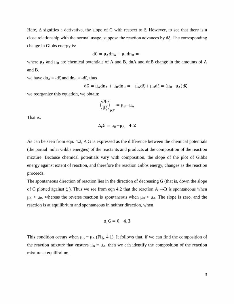
This condition occurs when μB = μA (Fig. 4.1). It follows that, if we can find the composition of

the reaction mixture that ensures μB = μA, then we can identify the composition of the reaction

mixture at equilibrium.

4

Fig. 6.1 As the reaction advances (represented by motion from left to right along the horizontal

axis) the slope of the Gibbs energy changes. Equilibrium corresponds to zero slope, at the foot of

the valley.

Note that the chemical potential is now fulfilling the role its name suggests: it represents the

potential for chemical change, and equilibrium is attained when these potentials are in balance.

4.1.2 Exergonic and endergonic reactions

We can express the spontaneity of a reaction at constant temperature and pressure in terms of the

reaction Gibbs energy:

If ΔrG < 0, the forward reaction is spontaneous.

If ΔrG > 0, the reverse reaction is spontaneous.

If ΔrG = 0, the reaction is at equilibrium.

A reaction for which ΔrG < 0 is called exergonic (i.e., workproducing). The name signifies that,

because the process is spontaneous, it can be used to drive another process, such as another

reaction, or used to do non-expansion work.

5

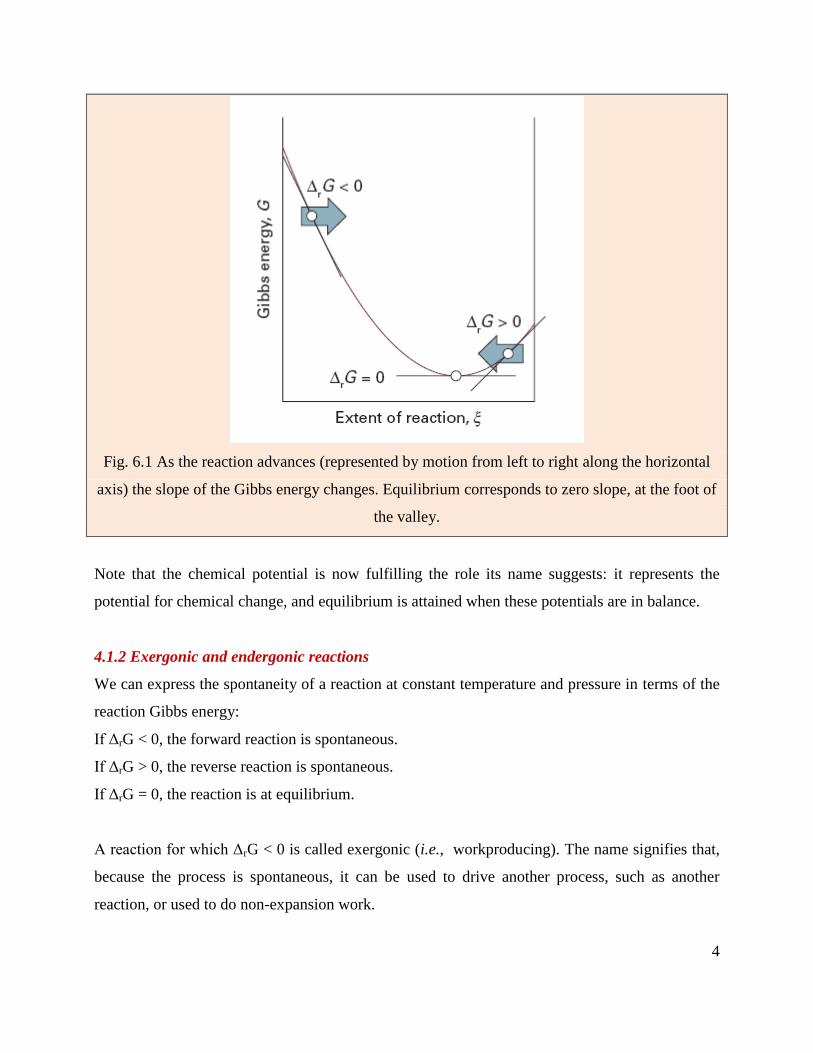
Brief illustration

A simple mechanical analogy is a pair of weights joined by a string (Fig. 4.2): the lighter of the

pair of weights will be pulled up as the heavier weight falls down.

Fig. 4.2 If two weights are coupled as shown here, then the heavier weight will move the lighter

weight in its non-spontaneous direction: overall, the process is still spontaneous. The weights are

the analogues of two chemical reactions: a reaction with a large negative ΔG can force another

reaction with a less negative ΔG to run in its non-spontaneous direction.

Although the lighter weight has a natural tendency to move downward, its coupling to the heavier

weight results in it being raised.

Brief illustration

In biological cells, the oxidation of carbohydrates act as the heavy weight that drives other

reactions forward and results in the formation of proteins from amino acids, muscle contraction,

and brain activity.

A reaction for which ΔrG > 0 is called endergonic (i.e., work-consuming). The reaction can be

made to occur only by doing work on it.

Brief illustration

Eelectrolyzing water to reverse its spontaneous formation reaction.

6

4.2 The description of equilibrium

In this section, we see how to apply thermodynamics to the description of chemical equilibrium.

4.2.1 Perfect gas equilibria

The chemical potential expression of a perfect gas is:

𝜇 = 𝜇° + 𝑅𝑇 ln 𝑝 ,𝑤ℎ𝑒𝑟𝑒 𝑝 𝑖𝑛𝑡𝑒𝑟𝑝𝑟𝑒𝑡𝑒𝑑 𝑎𝑠 𝑝/𝑝°

When A and B are perfect gases we can use the potential chemical expression to write:

∆rG = μB−μA = (𝜇𝐵° + 𝑅𝑇 ln pB) − (𝜇𝐴

° + 𝑅𝑇 ln pA)

∆rG = ∆rG° + 𝑅𝑇 ln

pBpA 𝟒. 𝟒

where, ∆rG° = 𝜇𝐵

° − 𝜇𝐴° , and 𝑅𝑇 ln pB − 𝑅𝑇 ln pA = 𝑅𝑇 ln

pB

pA

Denote the ratio of partial pressures by Q = pB/pA, we obtain

∆rG = ∆rG° + 𝑅𝑇 lnQ 𝑤ℎ𝑒𝑟𝑒 𝑄 =

pBpA 𝟒. 𝟓

The ratio Q is a reaction quotient (حاصل التفاعل) ( 0 ≤ Q ≤ ∞). It is 0 when pB = 0 (corresponding to

pure A), infinity (∞) when pA = 0 (corresponding to pure B).

The standard reaction Gibbs energy, ΔrG°, is defined (like the standard reaction enthalpy) as the

difference in the standard molar Gibbs energies of the reactants and products.

For our reaction

∆rG° = Gm

° (B) − Gm° (A) = μB

° − μA° 𝟒. 𝟔

Note that in the definition of ΔrG°, the Δr has its normal meaning as the difference ‘products –

reactants’. In chapter 3, we saw that the difference in standard molar Gibbs energies of the

products and reactants is equal to the difference in their standard Gibbs energies of formation, so

in practice we calculate ΔrG° from

∆rG° = ΔGf

°(B) − ΔGf°(A) 𝟒. 𝟕

At equilibrium ΔrG = 0. The ratio of partial pressures at equilibrium is denoted K, and eqn 4.5

becomes:

0 = ∆rG° + 𝑅𝑇 ln K

7

we rearrange to

𝑅𝑇 lnK = −∆rG° 𝐾 = (

pBpA)𝑒𝑞

𝟒. 𝟖

This relation is a special case of one of the most important equations in chemical

thermodynamics: it is the link between tables of thermodynamic data, such as those in the Data

section and the chemically important equilibrium constant, K.

In molecular terms, the minimum in the Gibbs energy, which corresponds to ΔrG = 0, stems from

the Gibbs energy of mixing of the two gases.

To see the role of mixing, consider the reaction A →B. If only the enthalpy were important, then

H and therefore G would change linearly from its value for pure reactants to its value for pure

products. The slope of this straight line is a constant and equal to ΔrG° at all stages of the reaction

and there is no intermediate minimum in the graph (Fig. 4.3).

Fig. 4.3 If the mixing of reactants and products is ignored, then the Gibbs energy changes linearly

from its initial value (pure reactants) to its final value (pure products) and the slope of the line is

ΔrG°. However, as products are produced, there is a further contribution to the Gibbs energy

arising from their mixing (lowest curve). The sum of the two contributions has a minimum. That

minimum corresponds to the equilibrium composition of the system.

8

However, when we take entropy into account, there is an additional contribution to the Gibbs

energy that is given by the expression: ΔmixG = nRT(xAln xA + xBlnxB)). This expression makes a

U-shaped contribution to the total change in Gibbs energy.

As can be seen from Fig. 4.3, when it is included there is an intermediate minimum in the total

Gibbs energy, and its position corresponds to the equilibrium composition of the reaction

mixture.

We see from eqn 4.8 that, when ΔrG° > 0, K < 1. Therefore, at equilibrium the partial pressure of

A exceeds that of B, which means that the reactant A is favoured in the equilibrium.

When ΔrG° < 0, K > 1, so at equilibrium the partial pressure of B exceeds that of A. Now the

product B is favoured in the equilibrium.

4.2.2 The general case of a reaction

The eqn 4.4 can be extend to a general reaction. A chemical reaction may be expressed

symbolically in terms of stoichiometric numbers as:

∑𝝂𝑱𝑱

𝑱 = 𝟎 𝟒. 𝟗

where J denotes the substances and the νJ are the corresponding stoichiometric numbers in the

chemical equation (A stoichiometric number is positive for products and negative for reactants).

Brief illustration

For instance, in the reaction

2 A + B→3 C + D

We have νA=−2, νB=−1, νC=+3, and νD=+1.

We define the extent of reaction ξ so that, if it changes by Δξ, then the change in the amount of

any species J is νJΔξ. With these points in mind and with the reaction Gibbs energy, ΔrG, defined

in the same way as before (eqn 4.1) we show in the following Justification that the Gibbs energy

of reaction can always be written:

∆𝐫𝐆 = ∆𝐫𝐆° + 𝑹𝑻 𝐥𝐧𝐐 𝟒. 𝟏𝟎

where

9

∆𝐫𝐆° = ∑ 𝛎𝐉

𝐏𝐫𝐨𝐝𝐮𝐜𝐭𝐬

∆𝐟𝐆° − ∑ 𝛎𝐉

𝐑𝐞𝐚𝐜𝐭𝐚𝐧𝐭𝐬

∆𝐟𝐆° = ∑𝛎𝐉

𝐉

∆𝐟𝐆° 𝟒. 𝟏𝟏𝐚

Or

∆𝐫𝐆° = ∑𝛎𝐉

𝐉

∆𝐟𝐆°(𝐉) 𝟒. 𝟏𝟏𝐛

Q is the reaction quotient, it has the form:

𝑸 =𝐚𝐜𝐭𝐢𝐯𝐢𝐭𝐢𝐞𝐬 𝐨𝐟 𝐩𝐫𝐨𝐝𝐮𝐜𝐭𝐬

𝐚𝐜𝐭𝐢𝐯𝐢𝐭𝐢𝐞𝐬 𝐨𝐟 𝐩𝐫𝐨𝐝𝐮𝐜𝐭𝐬 𝟒. 𝟏𝟐𝒂

More formally,

𝑸 =∏𝒂𝑱𝝂𝑱

𝑱

𝟒. 𝟏𝟐𝐚

where the symbol Π denotes the product of what follows it. aJ is the activity of the substance J,

and νJ its corresponding stoichiometric coefficient (νJ is positive for products, and negative for

reactants).

Note: Recall that, for pure solids and liquids, the activity is 1, so such substances make no

contribution to Q even though they may appear in the chemical equation.

Brief illustration

Consider the reaction 2 A + 3 B →C + 2 D, in which case νA = −2, νB = −3, νC = +1, and νD = +2.

The reaction quotient is then

𝑄 = 𝑎𝐴−2𝑎𝐵

−3𝑎𝐶1𝑎𝐷

2 =𝑎𝐶1𝑎𝐷

2

𝑎𝐴2𝑎𝐵3

Justification 4.1 The dependence of the reaction Gibbs energy on the reaction quotient

Consider a reaction with stoichiometric numbers νJ. When the reaction advances by dξ, the

amounts of reactants and products change by dnJ = νJdξ.

The resulting infinitesimal change in the Gibbs energy at constant temperature and pressure is

10

dG =∑𝜇JJ

dnJ =∑νJJ

μJdζ = (∑νJJ

μJ)dζ

It follows that,

Δ𝑟𝐺 = (dG

dζ)𝑝,𝑇

=∑νJJ

μJ

The chemical potential μJ of a species J is related to its activity by:

μJ = 𝜇𝐽° + 𝑅𝑇 ln aJ

When this expression is substituted into the expression above for ΔrG we obtain:

Δ𝑟𝐺 =∑νJJ

𝜇𝐽°

⏞ Δ𝑟𝐺

°

+ 𝑅𝑇∑νJJ

ln aJ

Δ𝑟𝐺 = Δ𝑟𝐺° + 𝑅𝑇 ln∏𝑎𝐽

νJ

𝐽

⏞ Q

Δ𝑟𝐺 = Δ𝑟𝐺° + 𝑅𝑇 lnQ

Starting from eqn 4.10. At equilibrium, the slope of G is zero: ΔrG= 0. The activities then have

their equilibrium values and we can write

𝐊 = (∏𝐚𝐉𝛎𝐉

𝐉

)

𝐞𝐪𝐮𝐢𝐥𝐢𝐛𝐫𝐢𝐮𝐦

𝟒. 𝟏𝟑

This expression has the same form as Q but is evaluated using equilibrium activities.

Note: From now on, we shall not write the ‘equilibrium’ subscript explicitly, and will rely on the

context to make it clear that for K we use equilibrium values and for Q we use the values at the

specified stage of the reaction.

11

An equilibrium constant K expressed in terms of activities (or fugacities) is called a

thermodynamic equilibrium constant. Note that, because activities are dimensionless numbers,

the thermodynamic equilibrium constant is also dimensionless.

In elementary applications, the activities that occur in eqn 4.13 are often replaced by:

molalities, by replacing aJ by bJ/b° where b° = 1 mol kg−1

molar concentrations, by replacing aJ by [J]/c°, where c° = 1 mol dm−3

partial pressures, by replacing aJ by pJ/p°, where p° = 1 bar

Note: In such cases, the resulting expressions are only approximations. The approximation is

particularly severe for electrolyte solutions, for in them activity coefficients differ from 1 even in

very dilute solutions.

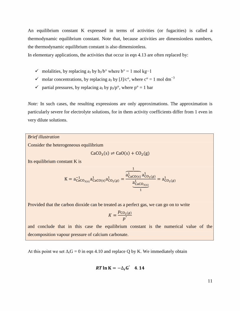
Brief illustration

Consider the heterogeneous equilibrium

CaCO3(s) ⇌ CaO(s) + CO2(g)

Its equilibrium constant K is

K = aCaCO3(s)−1 aCaCO(s)

1 aCO2(𝑔)1 =

aCaCO(s)1⏞ 1

aCO2(𝑔)1

aCaCO3(s)1⏟

1

= aCO2(𝑔)1

Provided that the carbon dioxide can be treated as a perfect gas, we can go on to write

𝐾 =𝑝CO2(𝑔)

𝑝°

and conclude that in this case the equilibrium constant is the numerical value of the

decomposition vapour pressure of calcium carbonate.

At this point we set ΔrG = 0 in eqn 4.10 and replace Q by K. We immediately obtain

𝑹𝑻 𝐥𝐧𝐊 = −∆𝐫𝐆° 𝟒. 𝟏𝟒

12

This is an exact and highly important thermodynamic relation, for it enables us to calculate the

equilibrium constant of any reaction from tables of thermodynamic data, and hence to predict the

equilibrium composition of the reaction mixture.

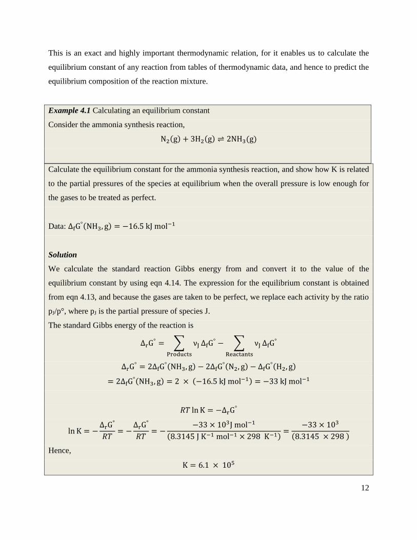
Example 4.1 Calculating an equilibrium constant

Consider the ammonia synthesis reaction,

N2(g) + 3H2(g) ⇌ 2NH3(g)

Calculate the equilibrium constant for the ammonia synthesis reaction, and show how K is related

to the partial pressures of the species at equilibrium when the overall pressure is low enough for

the gases to be treated as perfect.

Data: ∆fG°(NH3, g) = −16.5 kJ mol

−1

Solution

We calculate the standard reaction Gibbs energy from and convert it to the value of the

equilibrium constant by using eqn 4.14. The expression for the equilibrium constant is obtained

from eqn 4.13, and because the gases are taken to be perfect, we replace each activity by the ratio

pJ/p°, where pJ is the partial pressure of species J.

The standard Gibbs energy of the reaction is

∆rG° = ∑ νJ

Products

∆fG° − ∑ νJ

Reactants

∆fG°

∆rG° = 2∆fG

°(NH3, g) − 2∆fG°(N2, g) − ∆fG

°(H2, g)

= 2∆fG°(NH3, g) = 2 × (−16.5 kJ mol

−1) = −33 kJ mol−1

𝑅𝑇 lnK = −∆rG°

ln K = −∆rG

°

𝑅𝑇= −

∆rG°

𝑅𝑇= −

−33 × 103J mol−1

(8.3145 J K−1 mol−1 × 298 K−1)=

−33 × 103

(8.3145 × 298 )

Hence,

K = 6.1 × 105

13

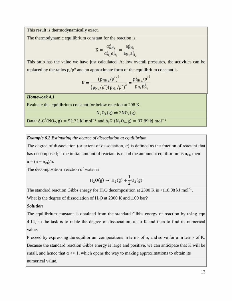
This result is thermodynamically exact.

The thermodynamic equilibrium constant for the reaction is

K =𝑎𝑁𝐻32

𝑎𝑁21 𝑎𝐻2

3 =aNH32

aN2aH23

This ratio has the value we have just calculated. At low overall pressures, the activities can be

replaced by the ratios pJ/p° and an approximate form of the equilibrium constant is

K =(pNH3/𝑝

°)2

(pN2/𝑝°)(pH2/𝑝

°)3 =

𝑝NH32 /𝑝°

2

pN2𝑝H23

Homework 4.1

Evaluate the equilibrium constant for below reaction at 298 K.

N2O4(g) ⇌ 2NO2(g)

Data: ∆fG°(NO2, g) = 51.31 kJ mol

−1 and ∆fG°(N2O4, g) = 97.89 kJ mol

−1

Example 6.2 Estimating the degree of dissociation at equilibrium

The degree of dissociation (or extent of dissociation, α) is defined as the fraction of reactant that

has decomposed; if the initial amount of reactant is n and the amount at equilibrium is neq, then

α = (n − neq)/n.

The decomposition reaction of water is

H2O(g) → H2(g) +1

2O2(g)

The standard reaction Gibbs energy for H2O decomposition at 2300 K is +118.08 kJ mol−1

.

What is the degree of dissociation of H2O at 2300 K and 1.00 bar?

Solution

The equilibrium constant is obtained from the standard Gibbs energy of reaction by using eqn

4.14, so the task is to relate the degree of dissociation, α, to K and then to find its numerical

value.

Proceed by expressing the equilibrium compositions in terms of α, and solve for α in terms of K.

Because the standard reaction Gibbs energy is large and positive, we can anticipate that K will be

small, and hence that α << 1, which opens the way to making approximations to obtain its

numerical value.

14

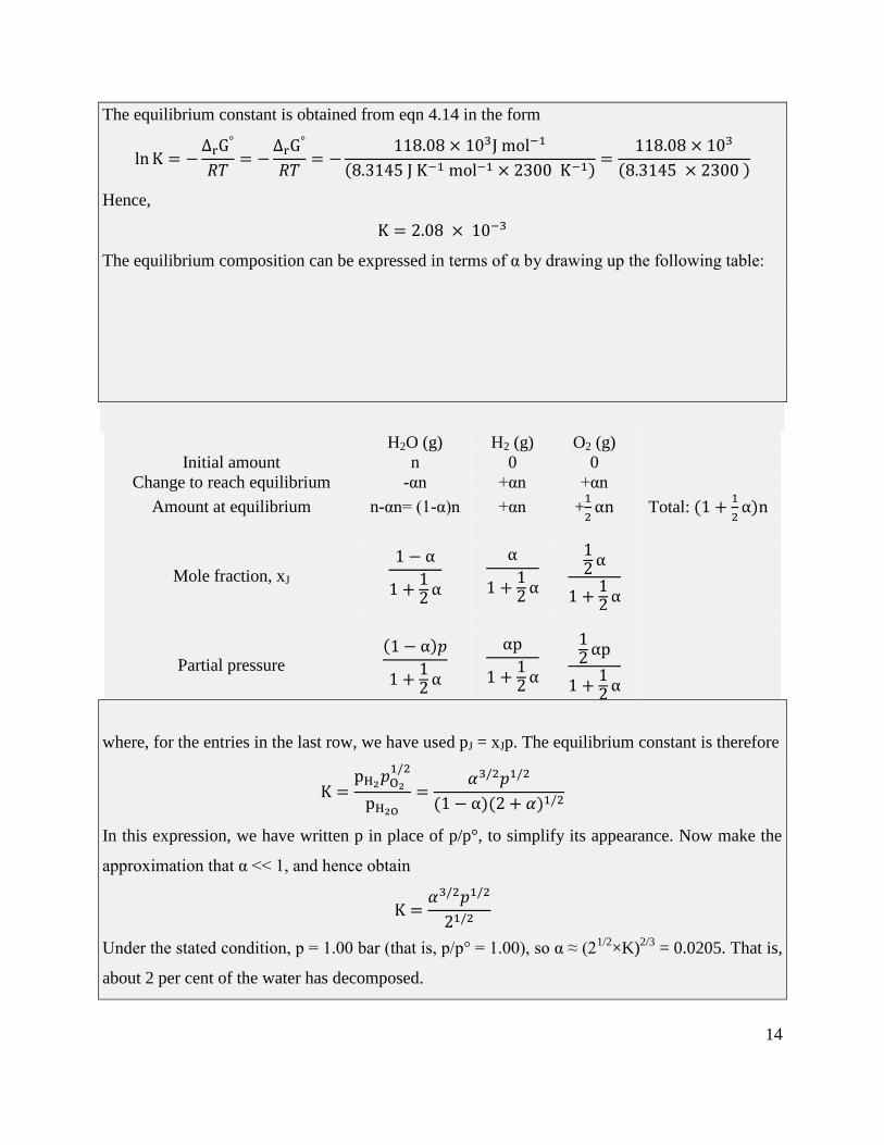
The equilibrium constant is obtained from eqn 4.14 in the form

ln K = −∆rG

°

𝑅𝑇= −

∆rG°

𝑅𝑇= −

118.08 × 103J mol−1

(8.3145 J K−1 mol−1 × 2300 K−1)=

118.08 × 103

(8.3145 × 2300 )

Hence,

K = 2.08 × 10−3

The equilibrium composition can be expressed in terms of α by drawing up the following table:

H2O (g) H2 (g) O2 (g)

Initial amount n 0 0

Change to reach equilibrium -αn +αn +αn

Amount at equilibrium n-αn= (1-α)n +αn +1

2αn Total: (1 +

1

2α)n

Mole fraction, xJ 1 − α

1 +12α

α

1 +12α

12α

1 +12α

Partial pressure (1 − α)𝑝

1 +12α

αp

1 +12α

12αp

1 +12α

where, for the entries in the last row, we have used pJ = xJp. The equilibrium constant is therefore

K =pH2𝑝O2

1/2

pH2O=

𝛼3/2𝑝1/2

(1 − α)(2 + 𝛼)1/2

In this expression, we have written p in place of p/p°, to simplify its appearance. Now make the

approximation that α << 1, and hence obtain

K =𝛼3/2𝑝1/2

21/2

Under the stated condition, p = 1.00 bar (that is, p/p° = 1.00), so α ≈ (21/2

×K)2/3

= 0.0205. That is,

about 2 per cent of the water has decomposed.

15

Homework 4.2

Given that the standard Gibbs energy of reaction at 2000 K is +135.2 kJ mol−1

for the same

reaction (Example 4.2), suppose that steam at 200 kPa is passed through a furnace tube at that

temperature. Calculate the mole fraction of O2 present in the output gas stream.

4.2.3. The relation between equilibrium constants

Equilibrium constants in terms of activities are exact, but it is often necessary to relate them to

concentrations. Formally, we need to know the activity coefficients, and then to use

𝑎𝐽 = 𝛾𝐽𝑥𝐽; 𝑎𝐽 = 𝛾𝐽 𝑏𝐽 𝑏°⁄ ; 𝑎𝐽 = 𝛾𝐽 [𝐽] 𝑐

°⁄ ;

where xJ is a mole fraction, bJ is a molality, and [J] is a molar concentration.

Example:

If we were interested in the composition in terms of molality for an equilibrium of the form:

A + B ⇌ C + D

where all four species are solutes, we would write

𝐊 =𝐚𝐂𝐚𝐃𝐚𝐀𝐚𝐁

=𝛄𝐂𝛄𝐃𝛄𝐀𝛄𝐁

∗𝐛𝐂𝐛𝐃𝐛𝐀𝐛𝐁

= 𝐊𝛄𝐊𝐛 𝟒. 𝟏𝟓

The activity coefficients must be evaluated at the equilibrium composition of the mixture (for

instance, by using one of the Debye–Hückel expressions), which may involve a complicated

calculation, because the activity coefficients are known only if the equilibrium composition is

already known. In elementary applications, and to begin the iterative calculation of the

concentrations in a real example, the assumption is often made that the activity coefficients are

all so close to unity that Kγ = 1. Then we obtain the result widely used in elementary chemistry

that K ≈ Kb, and equilibria are discussed in terms of molalities (or molar concentrations)

themselves.

A special case arises when we need to express the equilibrium constant of a gas-phase reaction in

terms of molar concentrations instead of the partial pressures that appear in the thermodynamic

equilibrium constant. Provided we can treat the gases as perfect, the pJ that appear in K can be

replaced by [J]RT, and

16

K =∏(aJ)νJ

J

=∏[𝐽]νJ

J

(𝑅𝑇

𝑝°)νJ

=∏[𝐽]νJ

J

×∏(𝑅𝑇

𝑝°)νJ

J

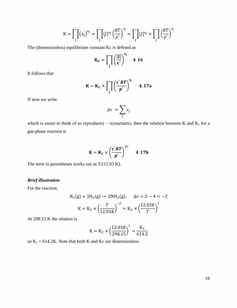
The (dimensionless) equilibrium constant Kc is defined as

𝐊𝐂 =∏([𝐉]

𝐜°)

𝛎𝐉

𝐉

𝟒. 𝟏𝟔

It follows that

𝐊 = 𝐊𝐂 ×∏(𝐜°𝑹𝑻

𝒑°)

𝛎𝐉

𝐉

𝟒. 𝟏𝟕𝐚

If now we write

𝛥𝜈 = ∑𝜈𝐽𝐽

which is easier to think of as ν(products) − ν(reactants), then the relation between K and Kc for a

gas-phase reaction is

𝐊 = 𝐊𝐂 × (𝐜°𝑹𝑻

𝒑°)

𝛥𝜈

𝟒. 𝟏𝟕𝐛

The term in parentheses works out as T/(12.03 K).

Brief illustration

For the reaction

N2(g) + 3H2(g) → 2NH3(g), ∆𝜈 = 2 − 4 = −2

K = KC × (𝑇

12.03𝐾)−2

= KC × (12.03𝐾

𝑇)2

At 298.15 K the relation is

K = KC × (12.03𝐾

298.15)2

=KC614.2

so Kc = 614.2K. Note that both K and Kc are dimensionless.

17

4.2.4 Molecular interpretation of the equilibrium constant

We can obtain a deeper insight into the origin and significance of the equilibrium constant by

considering the Boltzmann distribution of molecules over the available states of a system

composed of reactants and products.

When atoms can exchange partners, as in a reaction, the available states of the system include

arrangements in which the atoms are present in the form of reactants and in the form of products:

these arrangements have their characteristic sets of energy levels, but the Boltzmann distribution

does not distinguish between their identities, only their energies. The atoms distribute themselves

over both sets of energy levels in accord with the Boltzmann distribution (Fig. 4.4).

Fig. 4.4 The Boltzmann distribution of populations over the energy levels of two species A and B

with similar densities of energy levels; the reaction A →B is endothermic in this example. The

bulk of the population is associated with the species A, so that species is dominant at equilibrium.

At a given temperature, there will be a specific distribution of populations, and hence a specific

composition of the reaction mixture. It can be appreciated from the illustration that, if the

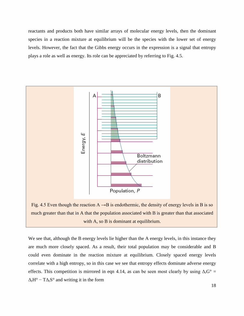
18

reactants and products both have similar arrays of molecular energy levels, then the dominant

species in a reaction mixture at equilibrium will be the species with the lower set of energy

levels. However, the fact that the Gibbs energy occurs in the expression is a signal that entropy

plays a role as well as energy. Its role can be appreciated by referring to Fig. 4.5.

Fig. 4.5 Even though the reaction A →B is endothermic, the density of energy levels in B is so

much greater than that in A that the population associated with B is greater than that associated

with A, so B is dominant at equilibrium.

We see that, although the B energy levels lie higher than the A energy levels, in this instance they

are much more closely spaced. As a result, their total population may be considerable and B

could even dominate in the reaction mixture at equilibrium. Closely spaced energy levels

correlate with a high entropy, so in this case we see that entropy effects dominate adverse energy

effects. This competition is mirrored in eqn 4.14, as can be seen most clearly by using ΔrG° =

ΔrH° − TΔrS° and writing it in the form

19

𝐊 = 𝒆−∆𝒓𝑯° 𝑹𝑻⁄ 𝒆∆𝒓𝑺

° 𝑹⁄ 𝟒. 𝟏𝟖

Note that a positive reaction enthalpy results in a lowering of the equilibrium constant (that is, an

endothermic reaction can be expected to have an equilibrium composition that favours the

reactants). However, if there is positive reaction entropy, then the equilibrium composition may

favour products, despite the endothermic character of the reaction.

4.2.3. Equilibria in biological systems

For biological systems, it is appropriate to adopt the biological standard state, in which aH+ = 10−7

and pH =−log aH+ = 7. The relation between the thermodynamic and biological standard Gibbs

energies of reaction for a reaction of the form

𝐑 + 𝛎𝐇+(𝐚𝐪) → 𝐏 𝟒. 𝟏𝟗𝐚

can be found by using the relation between the thermodynamic and biological standard values of

the chemical potential of hydrogen ions.

𝜇′ = 𝜇°′ − 7𝑅 ln 10

First, the general expression for the reaction Gibbs energy of this reaction is

Δ𝑟𝐺 = Δ𝑟𝐺° + 𝑅𝑇 ln

𝑎𝑃𝑎𝑅𝑎𝐻+

𝜈 = Δ𝑟𝐺° + 𝑅𝑇 ln

𝑎𝑃𝑎𝑅− 𝑅𝑇 ln 𝑎𝐻+

𝜈

In the biological standard state, both P and R are at unit activity (i.e., 𝑅𝑇 ln𝑎𝑃

𝑎𝑅= 0). Therefore,

by using ln x = ln 10 log x, this expression becomes

ΔrG = ΔrG° − νRT ln 10 log aH+ = ΔrG

° − νRT ln 10 pH

For the full specification of the biological state, we set pH = 7, and hence obtain

𝚫𝐫𝐆′ = 𝚫𝐫𝐆

° − 𝟕𝛎𝐑𝐓 𝐥𝐧𝟏𝟎 𝟒. 𝟏𝟗𝐛

Note: If hydrogen ions are not involved in the reaction (ν = 0). Thus, there is no difference

between the two standard values (ΔrG and ΔrG’).

20

Brief illustration

Consider the reaction NADH(aq) + H+(aq) → NAD

+(aq) + H2(g) at 37°C, for which ΔrG° =

−21.8 kJ mol−1

. It follows that, because ν = 1 and 7 ln 10 = 16.1,

ΔrG’ = −21.8 kJ mol−1

+ 16.1 × (8.3145 × 10−3

kJ K−1

mol−1

) × (310 K)

= +19.7 kJ mol−1

Note that the biological standard value is opposite in sign (in this example) to the thermodynamic

standard value: the much lower concentration of hydronium ions (by seven orders of magnitude)

at pH = 7 in place of pH = 0, has resulted in the reverse reaction becoming spontaneous under the

new standard conditions.

Homework 4.3

For a particular reaction of the form A → B + 2 H+ in aqueous solution, it was found that ΔrG° =

+20 kJ mol−1

at 28°C. Estimate the value of ΔrG’.

The response of equilibria to the conditions

Equilibria respond to changes in pressure, temperature, and concentrations of reactants and

products. The equilibrium constant for a reaction is not affected by the presence of a catalyst or

an enzyme (a biological catalyst).

4.3 How equilibria respond to changes of pressure

The equilibrium constant depends on the value of ΔrG°, which is defined at a single, standard

pressure. The value of ΔrG°, and hence of K, is therefore independent of the pressure at which the

equilibrium is actually established. In other words, at a given temperature K is a constant.

The conclusion that K is independent of pressure does not necessarily mean that the equilibrium

composition is independent of the pressure, and its effect depends on how the pressure is applied.

The pressure within a reaction vessel can be increased by injecting an inert gas into it. However,

so long as the gases are perfect, this addition of gas leaves all the partial pressures of the reacting

gases unchanged: the partial pressure of a perfect gas is the pressure it would exert if it were

alone in the container, so the presence of another gas has no effect. It follows that pressurization

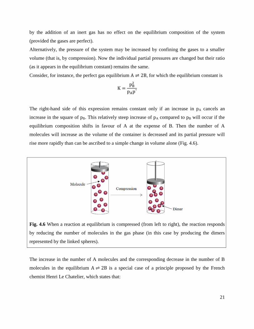
21

by the addition of an inert gas has no effect on the equilibrium composition of the system

(provided the gases are perfect).

Alternatively, the pressure of the system may be increased by confining the gases to a smaller

volume (that is, by compression). Now the individual partial pressures are changed but their ratio

(as it appears in the equilibrium constant) remains the same.

Consider, for instance, the perfect gas equilibrium A ⇌ 2B, for which the equilibrium constant is

K =pB2

pAp°

The right-hand side of this expression remains constant only if an increase in pA cancels an

increase in the square of pB. This relatively steep increase of pA compared to pB will occur if the

equilibrium composition shifts in favour of A at the expense of B. Then the number of A

molecules will increase as the volume of the container is decreased and its partial pressure will

rise more rapidly than can be ascribed to a simple change in volume alone (Fig. 4.6).

Fig. 4.6 When a reaction at equilibrium is compressed (from left to right), the reaction responds

by reducing the number of molecules in the gas phase (in this case by producing the dimers

represented by the linked spheres).

The increase in the number of A molecules and the corresponding decrease in the number of B

molecules in the equilibrium A ⇌ 2B is a special case of a principle proposed by the French

chemist Henri Le Chatelier, which states that:

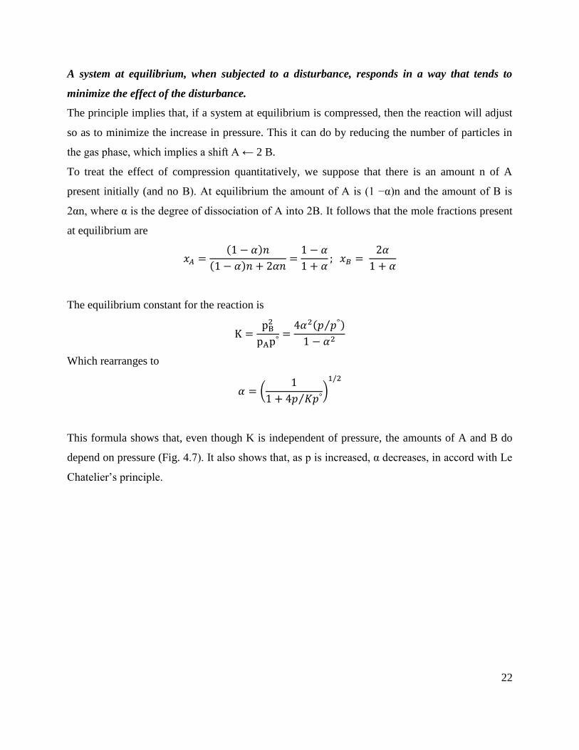
22

A system at equilibrium, when subjected to a disturbance, responds in a way that tends to

minimize the effect of the disturbance.

The principle implies that, if a system at equilibrium is compressed, then the reaction will adjust

so as to minimize the increase in pressure. This it can do by reducing the number of particles in

the gas phase, which implies a shift A ← 2 B.

To treat the effect of compression quantitatively, we suppose that there is an amount n of A

present initially (and no B). At equilibrium the amount of A is (1 −α)n and the amount of B is

2αn, where α is the degree of dissociation of A into 2B. It follows that the mole fractions present

at equilibrium are

𝑥𝐴 =(1 − 𝛼)𝑛

(1 − 𝛼)𝑛 + 2𝛼𝑛=1 − 𝛼

1 + 𝛼; 𝑥𝐵 =

2𝛼

1 + 𝛼

The equilibrium constant for the reaction is

K =pB2

pAp°=4𝛼2(𝑝 𝑝°⁄ )

1 − 𝛼2

Which rearranges to

𝛼 = (1

1 + 4𝑝 𝐾𝑝°⁄)1/2

This formula shows that, even though K is independent of pressure, the amounts of A and B do

depend on pressure (Fig. 4.7). It also shows that, as p is increased, α decreases, in accord with Le

Chatelier’s principle.

23

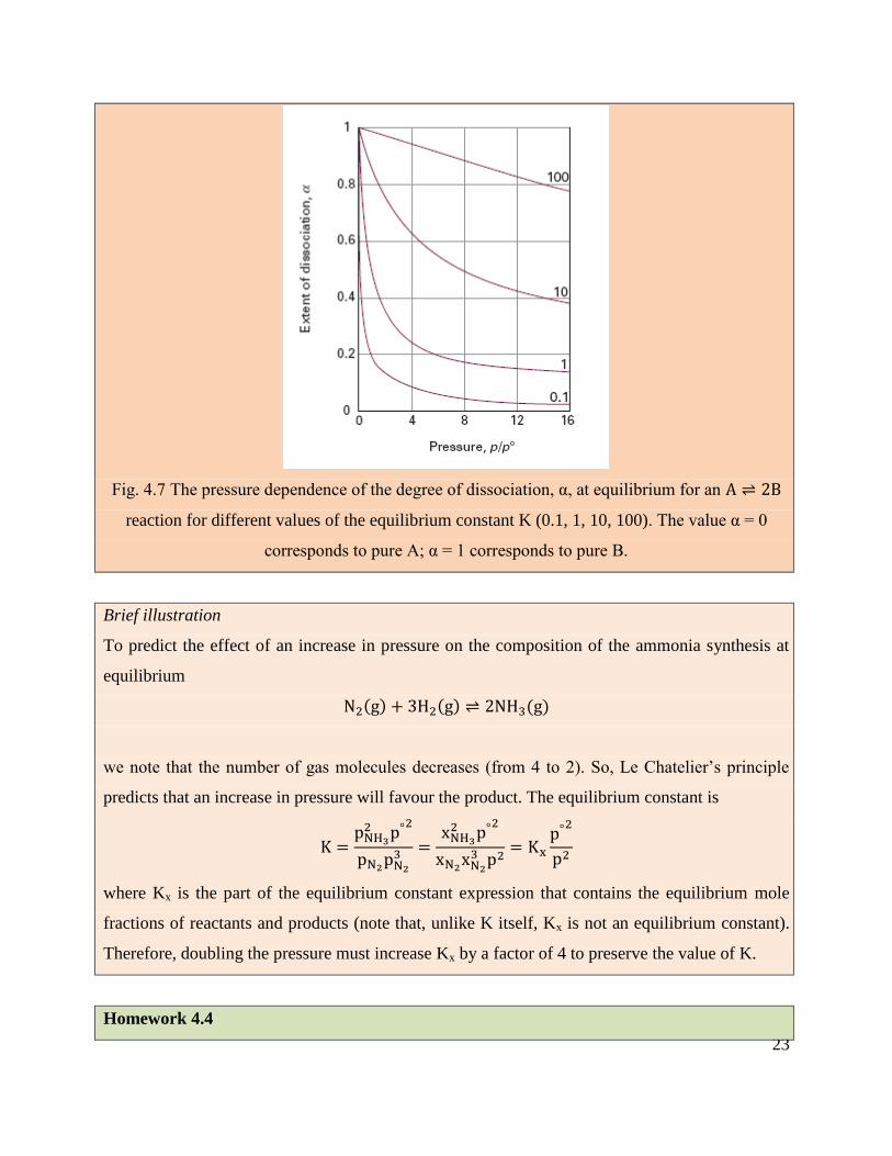
Fig. 4.7 The pressure dependence of the degree of dissociation, α, at equilibrium for an A ⇌ 2B

reaction for different values of the equilibrium constant K (0.1, 1, 10, 100). The value α = 0

corresponds to pure A; α = 1 corresponds to pure B.

Brief illustration

To predict the effect of an increase in pressure on the composition of the ammonia synthesis at

equilibrium

N2(g) + 3H2(g) ⇌ 2NH3(g)

we note that the number of gas molecules decreases (from 4 to 2). So, Le Chatelier’s principle

predicts that an increase in pressure will favour the product. The equilibrium constant is

K =pNH32 p°

2

pN2pN23 =

xNH32 p°

2

xN2xN23 p2

= Kxp°2

p2

where Kx is the part of the equilibrium constant expression that contains the equilibrium mole

fractions of reactants and products (note that, unlike K itself, Kx is not an equilibrium constant).

Therefore, doubling the pressure must increase Kx by a factor of 4 to preserve the value of K.

Homework 4.4

24

Predict the effect of a tenfold pressure increase on the equilibrium composition of the reaction.

3 N2(g) + H2(g)→2 N3H(g)

4.4 The response of equilibria to changes of temperature

Le Chatelier’s principle predicts that a system at equilibrium will tend to shift in the endothermic

direction if the temperature is raised, for then energy is absorbed as heat and the rise in

temperature is opposed. Conversely, an equilibrium can be expected to shift in the exothermic

direction if the temperature is lowered, for then energy is released and the reduction in

temperature is opposed. These conclusions can be summarized as follows:

Exothermic reactions: increased temperature favours the reactants.

Endothermic reactions: increased temperature favours the products.

We shall now justify these remarks and see how to express the changes quantitatively.

4.4.1 The van ’t Hoff equation

The van’t Hoff equation, which is derived in the Justification below, is an expression for the

slope of a plot of the equilibrium constant (specifically, ln K) as a function of temperature. It may

be expressed in either of two ways:

(𝐚) 𝐝 𝐥𝐧𝐊

𝐝𝐓=∆𝐫𝐇

°

𝐑𝐓𝟐 (𝐛)

𝐝 𝐥𝐧𝐊

𝐝(𝟏 𝐓⁄ )= −

∆𝐫𝐇°

𝐑 𝟒. 𝟐𝟏

Justification 4.2 The van’t Hoff equation

From eqn 4.14, we know that

ln K = −∆rG

°

RT

Differentiation of ln K with respect to temperature then gives:

d lnK

dT= −

1

R

𝑑(∆rG°/𝑇)

dT

The differentials are complete (that is, they are not partial derivatives) because K and ΔrG°

depend only on temperature, not on pressure.

To develop this equation we use the Gibbs–Helmholtz equation giving in the form

25

𝑑 (∆rG

°

𝑇 )

dT= −

∆rH°

T2

where ΔrH° is the standard reaction enthalpy at the temperature T. Combining the two equations

gives the van’t Hoff equation, eqn 4.21a. The second form of the equation is obtained by noting

that

d (1T)

dT−1

T2, so dT = −T2d (

1

T)

It follows that eqn 4.21a can be rewritten as

−d ln K

T2d(1T)=∆rH

°

RT2

which simplifies into eqn 4.21b.

Equation 4.21a shows that dln K/dT < 0 (and therefore that dK/dT < 0) for a reaction that is

exothermic under standard conditions (ΔrH° < 0). A negative slope means that lnK, and therefore

K itself, decreases as the temperature rises. Therefore, as asserted above, in the case of an

exothermic reaction the equilibrium shifts away from products. The opposite occurs in the case of

endothermic reactions.

Insight into the thermodynamic basis of this behaviour comes from the expression ΔrG° = ΔrH° −

TΔrS° written in the form −ΔrG°/T = −ΔrH°/T + ΔrS°. When the reaction is exothermic, −ΔrH°/T

corresponds to a positive change of entropy of the surroundings and favours the formation of

products. When the temperature is raised, −ΔrH°/T decreases, and the increasing entropy of the

surroundings has a less important role. As a result, the equilibrium lies less to the right. When the

reaction is endothermic, the principal factor is the increasing entropy of the reaction system. The

importance of the unfavourable change of entropy of the surroundings is reduced if the

temperature is raised (because then −ΔrH°/T is smaller), and the reaction is able to shift towards

products.

These remarks have a molecular basis that stems from the Boltzmann distribution of molecules

over the available energy levels. The typical arrangement of energy levels for an endothermic

reaction is shown in Fig. 4.8a.

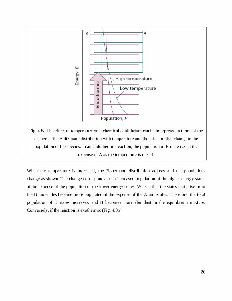
26

Fig. 4.8a The effect of temperature on a chemical equilibrium can be interpreted in terms of the

change in the Boltzmann distribution with temperature and the effect of that change in the

population of the species. In an endothermic reaction, the population of B increases at the

expense of A as the temperature is raised.

When the temperature is increased, the Boltzmann distribution adjusts and the populations

change as shown. The change corresponds to an increased population of the higher energy states

at the expense of the population of the lower energy states. We see that the states that arise from

the B molecules become more populated at the expense of the A molecules. Therefore, the total

population of B states increases, and B becomes more abundant in the equilibrium mixture.

Conversely, if the reaction is exothermic (Fig. 4.8b):

27

Fig. 4.8a The effect of temperature on a chemical equilibrium can be interpreted in terms of the

change in the Boltzmann distribution with temperature and the effect of that change in the

population of the species. In an exothermic reaction, the opposite happens.

Then an increase in temperature increases the population of the A states (which start at higher

energy) at the expense of the B states, so the reactants become more abundant.

28

4.4.2. The value of K at different temperatures

To find the value of the equilibrium constant at a temperature T2 in terms of its value K1 at

another temperature T1, we integrate eqn 4.21b between these two temperatures:

29

If we suppose that ΔrH° varies only slightly with temperature over the temperature range of

interest, then we may take it outside the integral. It follows that:

A brief illustration

To estimate the equilibrium constant for the synthesis of ammonia at 500 K from its value at 298

K (6.1 × 105 for the reaction as written in Example 4.1) we use the standard reaction enthalpy, by

using ΔrH° = 2ΔfH°(NH3,g), and assume that its value is constant over the range of temperatures.

Then, with ΔrH° = −92.2 kJ mol−1

, from eqn 4.23 we find

Homework

The equilibrium constant for N2O4(g) ⇌ NO2(g) at 25° is 0.15. Estimate its value at 100°C.

Equilibrium electrochemistry

The discussion has been general and applies to all reactions. One very special case is that of

reactions that take place in electrochemical cells. Electrochemical methods yield very precise

measurements of potential differences (‘voltages’), thus can be used to determine thermodynamic

properties of reactions that may be inaccessible by other methods.

Electrochemical cell: consists of two electrodes, or metallic conductors, in contact with an

electrolyte, an ionic conductor (which may be a solution, a liquid, or a solid).

An electrode and its electrolyte comprise an electrode compartment.

The two electrodes may share the same compartment.

30

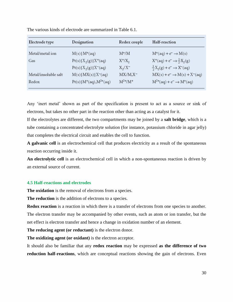
The various kinds of electrode are summarized in Table 6.1.

Any ‘inert metal’ shown as part of the specification is present to act as a source or sink of

electrons, but takes no other part in the reaction other than acting as a catalyst for it.

If the electrolytes are different, the two compartments may be joined by a salt bridge, which is a

tube containing a concentrated electrolyte solution (for instance, potassium chloride in agar jelly)

that completes the electrical circuit and enables the cell to function.

A galvanic cell is an electrochemical cell that produces electricity as a result of the spontaneous

reaction occurring inside it.

An electrolytic cell is an electrochemical cell in which a non-spontaneous reaction is driven by

an external source of current.

4.5 Half-reactions and electrodes

The oxidation is the removal of electrons from a species.

The reduction is the addition of electrons to a species.

Redox reaction is a reaction in which there is a transfer of electrons from one species to another.

The electron transfer may be accompanied by other events, such as atom or ion transfer, but the

net effect is electron transfer and hence a change in oxidation number of an element.

The reducing agent (or reductant) is the electron donor.

The oxidizing agent (or oxidant) is the electron acceptor.

It should also be familiar that any redox reaction may be expressed as the difference of two

reduction half-reactions, which are conceptual reactions showing the gain of electrons. Even

31

reactions that are not redox reactions may often be expressed as the difference of two reduction

half-reactions.

The reduced and oxidized species in a half-reaction form a redox couple. In general, redox

couple is written as Ox/Red and the corresponding reduction half-reaction as:

𝐎𝐱 + 𝛎𝐞− → 𝐑𝐞𝐝 𝟒. 𝟐𝟒

Brief solution

The dissolution of silver chloride in water AgCl(s) → Ag+(aq) + Cl

−(aq), which is not a redox

reaction, can be expressed as the difference of the following two reduction half-reactions:

AgCl(s) + e−→Ag(s) + Cl

−(aq)

Ag+(aq) + e

−→Ag(s)

The redox couples are AgCl/Ag, Cl− and Ag

+/Ag, respectively.

Homework

Express the formation of H2O from H2 and O2 in acidic solution (a redox reaction) as the

difference of two reduction half-reactions.

We shall often find it useful to express the composition of an electrode compartment in terms of

the reaction quotient, Q, for the half-reaction. This quotient is defined like the reaction quotient

for the overall reaction, but the electrons are ignored because they are stateless.

Brief illustration

Consider reduction of O2 to H2O in acid solution

The reaction quotient Q is

The approximations used in the second step are that the activity of water is 1 (because the

solution is dilute) and the oxygen behaves as a perfect gas, so aO2 ≈ pO2/p°.

32

Homework

Write the half-reaction and the reaction quotient for a chlorine gas electrode.

The reduction and oxidation processes responsible for the overall reaction in a cell are separated

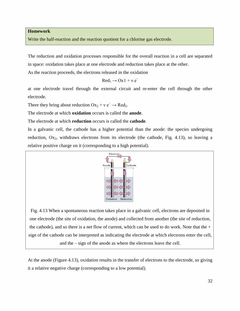
in space: oxidation takes place at one electrode and reduction takes place at the other.

As the reaction proceeds, the electrons released in the oxidation

Red1 → Ox1 + ν e−

at one electrode travel through the external circuit and re-enter the cell through the other

electrode.

There they bring about reduction Ox2 + ν e− → Red2.

The electrode at which oxidation occurs is called the anode.

The electrode at which reduction occurs is called the cathode.

In a galvanic cell, the cathode has a higher potential than the anode: the species undergoing

reduction, Ox2, withdraws electrons from its electrode (the cathode, Fig. 4.13), so leaving a

relative positive charge on it (corresponding to a high potential).

Fig. 4.13 When a spontaneous reaction takes place in a galvanic cell, electrons are deposited in

one electrode (the site of oxidation, the anode) and collected from another (the site of reduction,

the cathode), and so there is a net flow of current, which can be used to do work. Note that the +

sign of the cathode can be interpreted as indicating the electrode at which electrons enter the cell,

and the – sign of the anode as where the electrons leave the cell.

At the anode (Figure 4.13), oxidation results in the transfer of electrons to the electrode, so giving

it a relative negative charge (corresponding to a low potential).

33

4.6 Varieties of cells

* The simplest type of cell has a single electrolyte common to both electrodes (as in Fig. 4.13).

Fig. 4.13 When a spontaneous reaction takes place in a galvanic cell, electrons are deposited in

one electrode (the site of oxidation, the anode) and collected from another (the site of reduction,

the cathode), and so there is a net flow of current, which can be used to do work. Note that the +

sign of the cathode can be interpreted as indicating the electrode at which electrons enter the cell,

and the –sign of the anode as where the electrons leave the cell.

* In some cases it is necessary to immerse the electrodes in different electrolytes, as in the

‘Daniell cell’ in which the redox couple at one electrode is Cu2+

/Cu and at the other is Zn2+

/Zn

(Fig. 4.14).

Fig. 4.14 One version of the Daniell cell. The copper electrode is the cathode and the zinc

electrode is the anode. Electrons leave the cell from the zinc electrode and enter it again through

the copper electrode.

34

* In an electrolyte concentration cell: The electrode compartments are identical except for the

concentrations of the electrolytes.

* In an electrode concentration cell: The electrodes themselves have different concentrations,

either because they are gas electrodes operating at different pressures or because they are

amalgams (solutions in mercury) with different concentrations.

4.6.3 Liquid junction potentials

In a cell with two different electrolyte solutions in contact, as in the Daniell cell, there is an

additional source of potential difference across the interface of the two electrolytes. This potential

is called the liquid junction potential, 𝑬𝒍𝒋.

Another example of a junction potential is that between different concentrations of hydrochloric

acid. At the junction, the mobile H+ ions diffuse into the more dilute solution. The bulkier Cl

−

ions follow, but initially do so more slowly, which results in a potential difference at the junction.

The potential then settles down to a value such that, after that brief initial period, the ions diffuse

at the same rates.

Electrolyte concentration cells always have a liquid junction.

Electrode concentration cells do not.

The contribution of the liquid junction to the potential can be reduced (to about 1 to 2 mV) by

joining the electrolyte compartments through a salt bridge (Fig. 4.15).

Fig. 4.15 The salt bridge, essentially an inverted U-tube full of concentrated salt solution in a

jelly, has two opposing liquid junction potentials that almost cancel.

35

The reason for the success of the salt bridge is that, provided the ions dissolved in the jelly have

similar mobilities, then the liquid junction potentials at either end are largely independent of the

concentrations of the two dilute solutions, and so nearly cancel.

4.6.2 Notation

In the notation for cells, phase boundaries are denoted by a vertical bar. For example,

Pt(s)|H2(g)|HCl(aq)|AqCl(s)|Ag(s)

A liquid junction is denoted by ⋮, so the cell in Fig. 4.14 is denoted:

Zn(s)|ZnSO4(aq) ⋮ CuSO4(aq)|Cu(s)

A double vertical line, ||, denotes an interface for which it is assumed that the junction potential

has been eliminated. Thus, the cell in Fig. 4.15 is denoted:

Zn(s)|ZnSO4(aq)||CuSO4(aq)|Cu(s)

An example of an electrolyte concentration cell in which the liquid junction potential is assumed

to be eliminated is:

Pt(s)|H2(g)|HCl(aq,b1)||HCl(aq,b2)|H2(g)|Pt(s)

4.7 The cell potential

The current produced by a galvanic cell arises from the spontaneous chemical reaction taking

place inside it. The cell reaction is the reaction in the cell written on the assumption that the right-

hand electrode is the cathode, and hence that the spontaneous reaction is one in which reduction

is taking place in the right-hand compartment.

Later we see how to predict if the right-hand electrode is in fact the cathode; if it is, then the cell

reaction is spontaneous as written.

If the left-hand electrode turns out to be the cathode, then the reverse of the corresponding cell

reaction is spontaneous.

To write the cell reaction corresponding to a cell diagram, we first write the right-hand half-

reaction as a reduction (because we have assumed that to be spontaneous). Then we subtract from

it the left-hand reduction half-reaction (for, by implication, that electrode is the site of oxidation).

Thus, in the cell Zn(s)|ZnSO4(aq)||CuSO4(aq)|Cu(s)

36

The two electrodes and their reduction half-reactions are:

Right-hand electrode: Cu2+

(aq) + 2 e− → Cu(s)

Left-hand electrode: Zn2+

(aq) + 2 e → Zn(s)

Hence, the overall cell reaction is the difference:

Cu2+

( aq) + Zn(s) → Cu(s) + Zn2+

(aq)

4.7.1 The Nernst equation

A cell in which the overall cell reaction has not reached chemical equilibrium can do electrical

work as the reaction drives electrons through an external circuit.

The work that a given transfer of electrons can accomplish depends on the potential difference

between the two electrodes. When the potential difference is large, a given number of electrons

travelling between the electrodes can do a large amount of electrical work.

When the potential difference is small, the same number of electrons can do only a small amount

of work.

A cell in which the overall reaction is at equilibrium can do no work, and then the potential

difference is zero.

According to the discussion in chapter 3, we know that the maximum non-expansion work a

system can do is given by:

wadd,max = ΔG

In electrochemistry, the non-expansion work is identified with electrical work, the system is the

cell, and ΔG is the Gibbs energy of the cell reaction, ΔrG.

Maximum work is produced when a change occurs reversibly.

It follows that, to draw thermodynamic conclusions from measurements of the work that a cell

can do, we must ensure that the cell is operating reversibly. Moreover, we saw in Section 6.1a

that the reaction Gibbs energy is actually a property relating to a specified composition of the

reaction mixture.

Therefore, to make use of ΔrG we must ensure that the cell is operating reversibly at a specific,

constant composition. Both these conditions are achieved by measuring the cell potential when it

is balanced by an exactly opposing source of potential so that the cell reaction occurs reversibly,

the composition is constant, and no current flows: in effect, the cell reaction is poised for change,

37

but not actually changing. The resulting potential difference is called the cell potential, Ecell, of

the cell. As we show in the Justification below, the relation between the reaction Gibbs energy

and the cell potential is

−𝝂𝑭𝑬𝒄𝒆𝒍𝒍 = 𝜟𝒓𝑮 𝟒. 𝟐𝟓

where F is Faraday’s constant, F = eNA, and ν is the stoichiometric coefficient of the electrons in

the half-reactions into which the cell reaction can be divided. This equation is the key connection

between electrical measurements on the one hand and thermodynamic properties on the other. It

will be the basis of all that follows.

Justification 6.3 The relation between the cell potential and the reaction Gibbs energy

We consider the change in G when the cell reaction advances by an infinitesimal amount dξ at

some composition. From Justification 4.1 we can write (at constant temperature and pressure)

dG = ΔrGdξ

The maximum non-expansion (electrical) work that the reaction can do as it advances by dξ at

constant temperature and pressure is therefore

dwe = ΔrGdξ

This work is infinitesimal, and the composition of the system is virtually constant when it occurs.

Suppose that the reaction advances by dξ; then νdξ electrons must travel from the anode to the

cathode.

The total charge transported between the electrodes when this change occurs is −νeNAdξ (because

νdξ is the amount of electrons and the charge per mole of electrons is −eNA). Hence, the total

charge transported is −νFdξ because eNA = F.

The work done when an infinitesimal charge −νFdξ travels from the anode to the cathode is equal

to the product of the charge and the potential difference Ecell:

dwe = −νFEcelldξ

When we equate this relation to the one above (dwe = ΔrGdξ), the advancement dξ cancels, and

we obtain eqn 4.25.

38

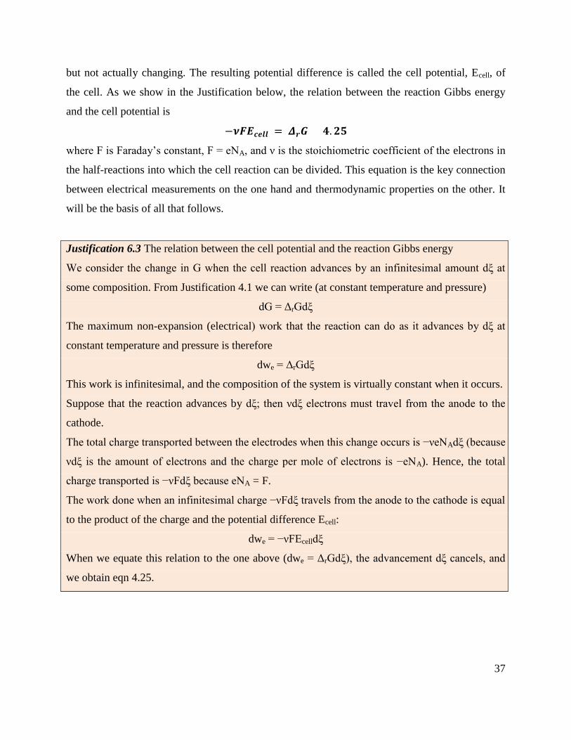
It follows from eqn 4.25 that, by knowing the reaction Gibbs energy at a specified composition,

we can state the cell potential at that composition. Note that a negative reaction Gibbs energy,

corresponding to a spontaneous cell reaction, corresponds to a positive cell potential.

Another way of looking at the content of eqn 4.25 is that it shows that the driving power of a cell

(that is, its potential) is proportional to the slope of the Gibbs energy with respect to the extent of

reaction.

It is plausible that a reaction that is far from equilibrium (when the slope is steep) has a strong

tendency to drive electrons through an external circuit (Fig. 4.16).

Fig. 4.16 A spontaneous reaction occurs in the direction of decreasing Gibbs energy and can be

expressed in terms of the cell potential, Ecell. The reaction is spontaneous as written (from left to

right on the illustration) when Ecell > 0. The reverse reaction is spontaneous when Ecell < 0. When

the cell reaction is at equilibrium, the cell potential is zero.

When the slope is close to zero (when the cell reaction is close to equilibrium), the cell potential

is small.

Brief illustration

Equation 4.25 provides an electrical method for measuring a reaction Gibbs energy at any

composition of the reaction mixture: we simply measure the cell potential and convert it to ΔrG.

Conversely, if we know the value of ΔrG at a particular composition, then we can predict the cell

potential. For example, if ΔrG = −1 × 102 kJ mol−1

and ν = 1, then

𝐸𝑐𝑒𝑙𝑙 = −Δ𝑟𝐺

𝜈𝐹= −

−1 × 105 J mol−1

1 × (6.6485 × 104C mol−1)= 1𝑉

39

We can go on to relate the cell potential to the activities of the participants in the cell reaction.

We know that the reaction Gibbs energy is related to the composition of the reaction mixture by

eqn 4.10 ((ΔrG=ΔrG° + RT ln Q)); it follows, on division of both sides by −νF, that

𝐸𝑐𝑒𝑙𝑙 = −Δ𝑟𝐺

°

𝜈𝐹−𝑅𝑇

𝜈𝐹ln𝑄

The first term on the right is written

𝑬𝒄𝒆𝒍𝒍° = −

𝚫𝒓𝑮°

𝝂𝑭 𝟒. 𝟐𝟔

and called the standard cell potential. That is, the standard cell potential is the standard reaction

Gibbs energy expressed as a potential difference (in volts).

It follows that

𝑬𝒄𝒆𝒍𝒍 = 𝑬𝒄𝒆𝒍𝒍° −

𝑹𝑻

𝝂𝑭𝐥𝐧𝑸 𝟒. 𝟐𝟕

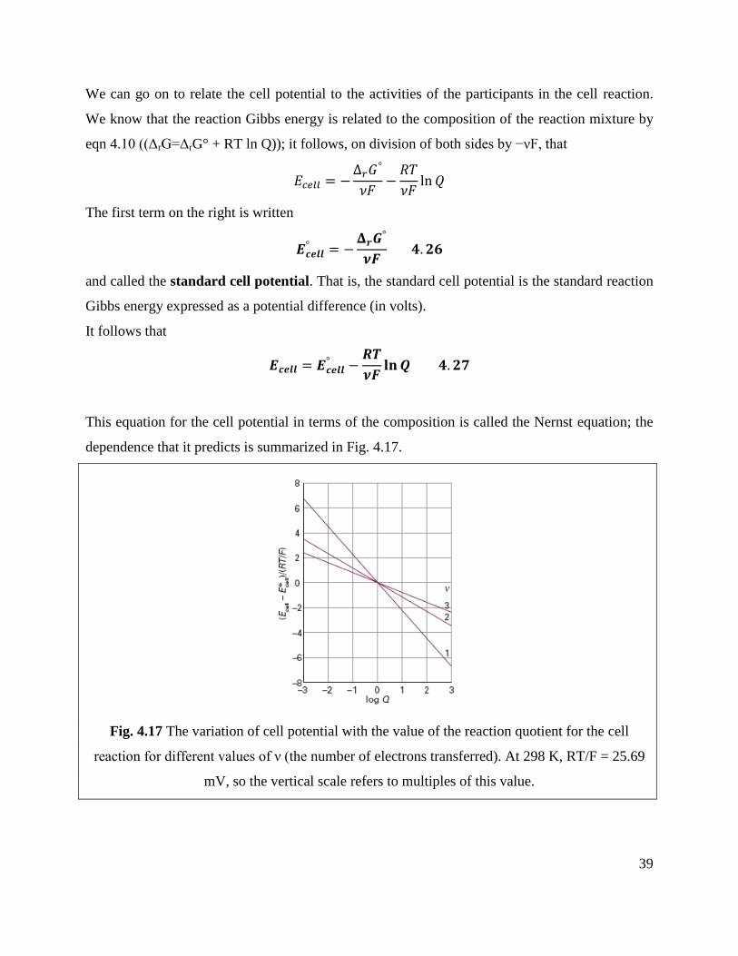
This equation for the cell potential in terms of the composition is called the Nernst equation; the

dependence that it predicts is summarized in Fig. 4.17.

Fig. 4.17 The variation of cell potential with the value of the reaction quotient for the cell

reaction for different values of ν (the number of electrons transferred). At 298 K, RT/F = 25.69

mV, so the vertical scale refers to multiples of this value.

40

One important application of the Nernst equation is to the determination of the pH of a solution

and, with a suitable choice of electrodes, of the concentration of other ions.

We see from eqn 4.27 that the standard cell potential (which will shortly move to centre stage of

the exposition) can be interpreted as the cell potential when all the reactants and products in the

cell reaction are in their standard states, for then all activities are 1, so Q = 1 and ln Q = 0.

However, the fact that the standard cell potential is merely a disguised form of the standard

reaction Gibbs energy (eqn 4.26) should always be kept in mind and underlies all its applications.

4.7.2 Cells at equilibrium

A special case of the Nernst equation has great importance in electrochemistry and provides a

link to the earlier part of the chapter. Suppose the reaction has reached equilibrium; then Q = K,

where K is the equilibrium constant of the cell reaction.

However, a chemical reaction at equilibrium cannot do work, and hence it generates:

𝝂𝑭𝑬𝒄𝒆𝒍𝒍°

𝑹𝑻= 𝐥𝐧𝑲 𝟒. 𝟐𝟖

This very important equation (which could also have been obtained more directly by substituting

eqn 4.26 into eqn 4.14) lets us predict equilibrium constants from measured standard cell

potentials. However, before we use it extensively, we need to establish a further result.

4.8 Standard electrode potentials

A galvanic cell is a combination of two electrodes each of which can be considered to make a

characteristic contribution to the overall cell potential. Although it is not possible to measure the

contribution of a single electrode, we can define the potential of one of the electrodes as zero and

then assign values to others on that basis. The specially selected electrode is the standard

hydrogen electrode (SHE):

𝐏𝐭(𝐬)|𝐇𝟐(𝐠)|𝐇+(𝐚𝐪)𝐄° = 𝟎 𝟔. 𝟐𝟗

at all temperatures. To achieve the standard conditions, the activity of the hydrogen ions must be

1 (that is, pH = 0) and the pressure (more precisely, the fugacity) of the hydrogen gas must be 1

bar.

41

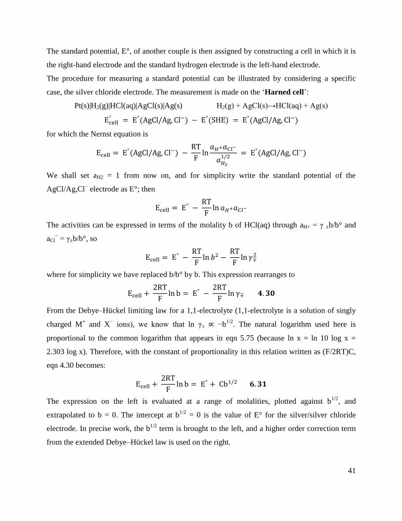
The standard potential, E°, of another couple is then assigned by constructing a cell in which it is

the right-hand electrode and the standard hydrogen electrode is the left-hand electrode.

The procedure for measuring a standard potential can be illustrated by considering a specific

case, the silver chloride electrode. The measurement is made on the ‘Harned cell’:

Pt(s)|H2(g)|HCl(aq)|AgCl(s)|Ag(s) H2(g) + AgCl(s)→HCl(aq) + Ag(s)

Ecell° = E°(AgCl/Ag, Cl−) − E°(SHE) = E°(AgCl/Ag, Cl−)

for which the Nernst equation is

Ecell = E°(AgCl/Ag, Cl−) −

RT

Fln𝑎𝐻+𝑎𝐶𝑙−

𝑎𝐻21/2

= E°(AgCl/Ag, Cl−)

We shall set aH2 = 1 from now on, and for simplicity write the standard potential of the

AgCl/Ag,Cl− electrode as E°; then

Ecell = E° −

RT

Fln 𝑎𝐻+𝑎𝐶𝑙−

The activities can be expressed in terms of the molality b of HCl(aq) through aH+ = γ ±b/b° and

aCl− = γ±b/b°, so

Ecell = E° −

RT

Fln 𝑏2 −

RT

Fln 𝛾∓

2

where for simplicity we have replaced b/b° by b. This expression rearranges to

Ecell + 2RT

Fln b = E° −

2RT

Fln γ∓ 𝟒. 𝟑𝟎

From the Debye–Hückel limiting law for a 1,1-electrolyte (1,1-electrolyte is a solution of singly

charged M+ and X

− ions), we know that ln γ± ∝ −b

1/2. The natural logarithm used here is

proportional to the common logarithm that appears in eqn 5.75 (because ln x = ln 10 log x =

2.303 log x). Therefore, with the constant of proportionality in this relation written as (F/2RT)C,

eqn 4.30 becomes:

Ecell + 2RT

Fln b = E° + Cb1/2 𝟔. 𝟑𝟏

The expression on the left is evaluated at a range of molalities, plotted against b1/2

, and

extrapolated to b = 0. The intercept at b1/2

= 0 is the value of E° for the silver/silver chloride

electrode. In precise work, the b1/2

term is brought to the left, and a higher order correction term

from the extended Debye–Hückel law is used on the right.

42

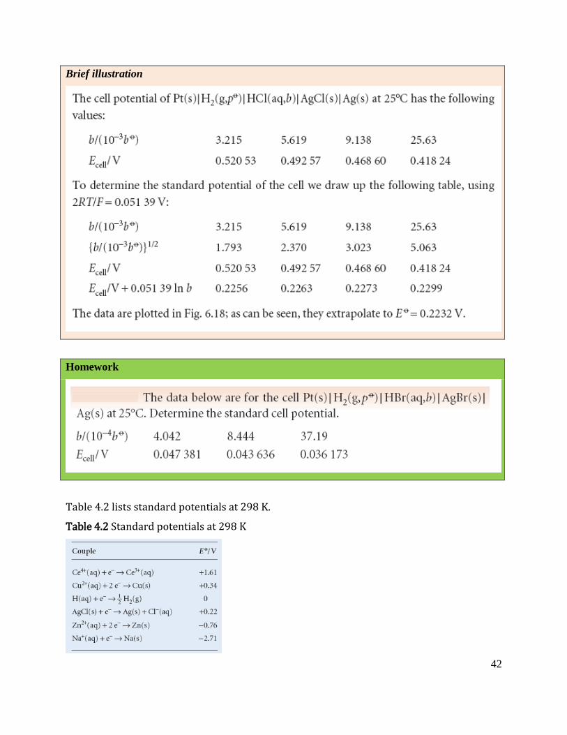
Brief illustration

Homework

Table 4.2 lists standard potentials at 298 K.

Table 4.2 Standard potentials at 298 K

43

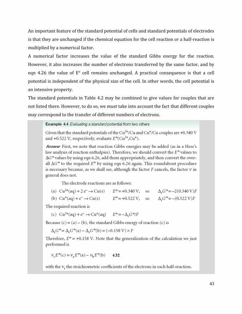
An important feature of the standard potential of cells and standard potentials of electrodes

is that they are unchanged if the chemical equation for the cell reaction or a half-reaction is

multiplied by a numerical factor.

A numerical factor increases the value of the standard Gibbs energy for the reaction.

However, it also increases the number of electrons transferred by the same factor, and by

eqn 4.26 the value of E° cell remains unchanged. A practical consequence is that a cell

potential is independent of the physical size of the cell. In other words, the cell potential is

an intensive property.

The standard potentials in Table 4.2 may be combined to give values for couples that are

not listed there. However, to do so, we must take into account the fact that different couples

may correspond to the transfer of different numbers of electrons.

44

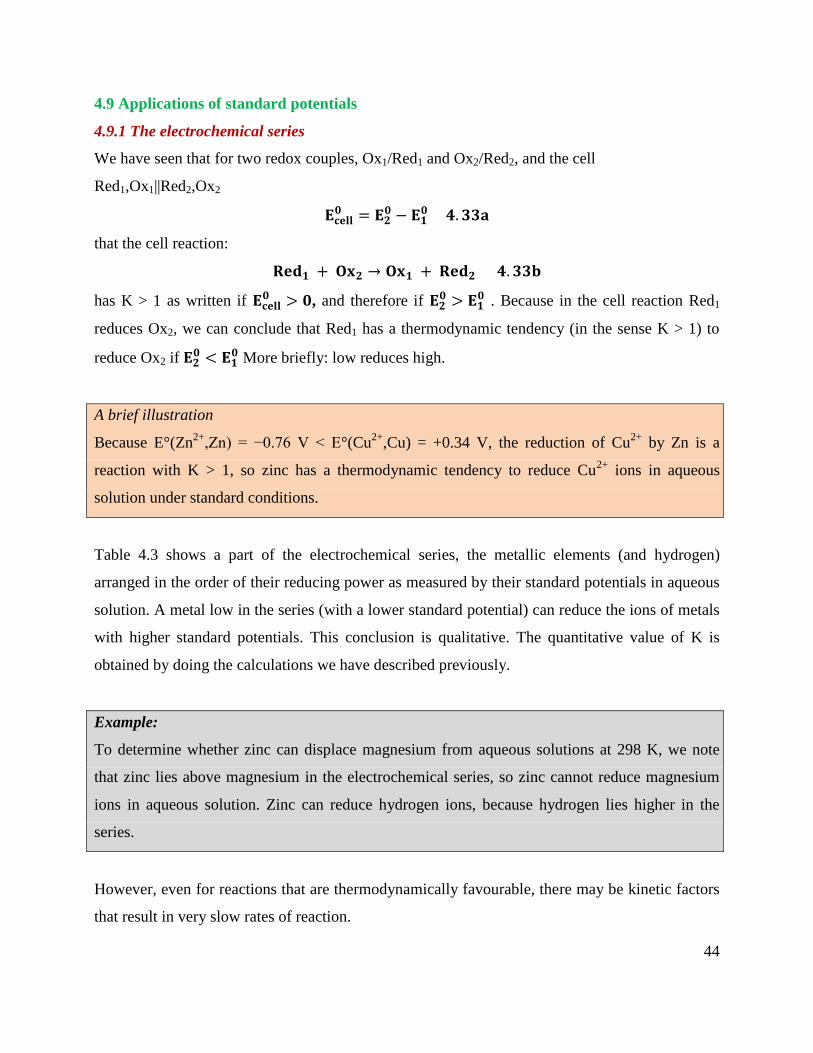
4.9 Applications of standard potentials

4.9.1 The electrochemical series

We have seen that for two redox couples, Ox1/Red1 and Ox2/Red2, and the cell

Red1,Ox1||Red2,Ox2

𝐄𝐜𝐞𝐥𝐥𝟎 = 𝐄𝟐

𝟎 − 𝐄𝟏𝟎 𝟒. 𝟑𝟑𝐚

that the cell reaction:

𝐑𝐞𝐝𝟏 + 𝐎𝐱𝟐 → 𝐎𝐱𝟏 + 𝐑𝐞𝐝𝟐 𝟒. 𝟑𝟑𝐛

has K > 1 as written if 𝐄𝐜𝐞𝐥𝐥𝟎 > 𝟎, and therefore if 𝐄𝟐

𝟎 > 𝐄𝟏𝟎 . Because in the cell reaction Red1

reduces Ox2, we can conclude that Red1 has a thermodynamic tendency (in the sense K > 1) to

reduce Ox2 if 𝐄𝟐𝟎 < 𝐄𝟏

𝟎 More briefly: low reduces high.

A brief illustration

Because E°(Zn2+

,Zn) = −0.76 V < E°(Cu2+

,Cu) = +0.34 V, the reduction of Cu2+

by Zn is a

reaction with K > 1, so zinc has a thermodynamic tendency to reduce Cu2+

ions in aqueous

solution under standard conditions.

Table 4.3 shows a part of the electrochemical series, the metallic elements (and hydrogen)

arranged in the order of their reducing power as measured by their standard potentials in aqueous

solution. A metal low in the series (with a lower standard potential) can reduce the ions of metals

with higher standard potentials. This conclusion is qualitative. The quantitative value of K is

obtained by doing the calculations we have described previously.

Example:

To determine whether zinc can displace magnesium from aqueous solutions at 298 K, we note

that zinc lies above magnesium in the electrochemical series, so zinc cannot reduce magnesium

ions in aqueous solution. Zinc can reduce hydrogen ions, because hydrogen lies higher in the

series.

However, even for reactions that are thermodynamically favourable, there may be kinetic factors

that result in very slow rates of reaction.

45

Table 4.3

4.9.2 The determination of activity coefficients

Once the standard potential of an electrode in a cell is known, we can use it to determine mean

activity coefficients by measuring the cell potential with the ions at the concentration of interest.

Example:

The mean activity coefficient of the ions in hydrochloric acid of molality b is obtained from eqn

4.30 in the form:

𝐥𝐧 𝛄∓ = 𝐄° − 𝐄𝐜𝐞𝐥𝐥𝟐𝐑𝐓/𝐅

− 𝐥𝐧𝐛 𝟒. 𝟑𝟒

46

4.9.3 The determination of equilibrium constants

The principal use for standard potentials is to calculate the standard potential of a cell formed

from any two electrodes. To do so, we subtract the standard potential of the left-hand electrode

from the standard potential of the right-hand electrode:

𝐄𝐜𝐞𝐥𝐥° = 𝐄°(𝐫𝐢𝐠𝐡𝐭) − 𝐄°(𝐫𝐢𝐠𝐡𝐭) 𝟒. 𝟑𝟓

Because ∆𝑟𝐺° = −𝜈𝐹Ecell

° , it then follows that, if the result gives Ecell° > 0, then the

corresponding cell reaction has K > 1.

Brief illustration

A disproportionation is a reaction in which a species is both oxidized and reduced. To study the

disproportionation 2 Cu+(aq)→Cu(s) + Cu

2+(aq) we combine the following electrodes:

Right-hand electrode: Cu(s)|Cu+(aq) Cu

+(aq) + e

−→Cu(aq) E° = +0.52 V

Left-hand electrode: Pt(s)|Cu2+(aq), Cu+(aq) Cu2+

(aq) + e−→Cu

+(s) E° = +0.16 V

where the standard potentials are measured at 298 K. The standard potential of the cell is

therefore

Ecell° = +0.52 V − 0.16 V = +0.36 V

We can now calculate the equilibrium constant of the cell reaction. Because ν = 1, from eqn 4.28,

ln 𝐾 =0.36 𝑉

0.025 × 693 𝑉=

0.36

0.025 × 693

Hence, K = 1.2 × 106.

4.9.4 The determination of thermodynamic functions

The standard potential of a cell is related to the standard reaction Gibbs energy through eqn 4.25

(Δ𝑟𝐺° = −𝜈𝐹Ecell

° ). Therefore, by measuring Ecell° we can obtain this important thermodynamic

quantity. Its value can then be used to calculate the Gibbs energy of formation of ions by using

the convention explained in Section 3.6.

Brief illustration

The cell reaction taking place in Pt(s)|H2|H+(aq)||Ag

+(aq)|Ag(s) Ecell

° = +0.7996 V 7

is

47

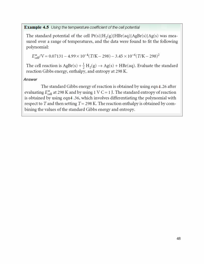
Ag+(aq) + H2(g) → H

+(aq) + Ag(s) ΔrG° = −ΔfG°(Ag+,aq)

Therefore, with ν = 1, we find ΔfG°(Ag+,aq) = −(−Ecell° ) = +77.15 kJ mol

−1.

The temperature coefficient of the standard cell potential, 𝑑Ecell

°

𝑑𝑇, gives the standard entropy of the

cell reaction. This conclusion follows from the thermodynamic relation (∂G/∂T)p = −S and eqn

4.26, which combine to give:

𝒅𝐄𝐜𝐞𝐥𝐥°

𝒅𝑻=𝚫𝒓𝑺

°

𝝂𝑭 𝟒. 𝟑𝟔

The derivative is complete (not partial) because E°, like ΔrG°, is independent of the pressure.

Hence, we have an electrochemical technique for obtaining standard reaction entropies and

through them the entropies of ions in solution. Finally, we can combine the results obtained so far

and use them to obtain the standard reaction enthalpy:

𝚫𝒓𝑯° = 𝚫𝒓𝑮

° + 𝑻𝚫𝒓𝑺° = 𝝂𝑭(𝐄𝐜𝐞𝐥𝐥

° − 𝑻𝒅𝐄𝐜𝐞𝐥𝐥

°

𝒅𝑻) 𝟒. 𝟑𝟕

This expression provides a non-calorimetric method for measuring ΔrH° and, through the

convention ΔfH°(H+,aq) = 0, the standard enthalpies of formation of ions in solution (Section

2.8). Thus, electrical measurements can be used to calculate all the thermodynamic properties

with which this chapter began.

48

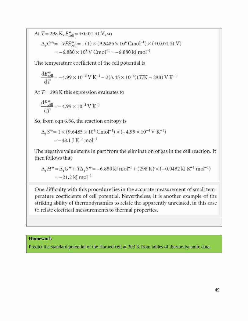
49

Homework

Predict the standard potential of the Harned cell at 303 K from tables of thermodynamic data.