chapter 4: cfd modelling and base case verification

CHAPTER 4: CFD MODELLING OF BASE CASE 70

CHAPTER 4: CFD MODELLING AND BASE CASE

VERIFICATION

The objective of this dissertation is to ultimately perform design optimisation of the

SEN using CFD modelling, in order to achieve an optimum SEN in the continuous

casting process. This will involve the set-up and solution of multiple CFD models.

The first step towards this goal is to model the base case (starting point of the

optimisation exercise), which is usually a current SEN design. As soon as confidence

in the CFD modelling process is achieved (by the end of this chapter), different SEN

designs can be evaluated for optimisation purposes (Chapter 5).

By the end of this chapter, the reader will be convinced that the methods followed to

model a typical SEN and mould set-up is reliable and will ensure correct CFD

solution flow fields, as these solutions are validated with water model experiments.

4.1 Approach: CFD modelling of base case design

A CFD model of any engineering flow application involves a number of inputs by the

user to be physically representative of the real flow situation. These inputs involve a

wide range of issues from grid generation (type of grid-elements, and geometric

simplifications, inter alia) to turbulence modelling (choice of models to use to

simulate physical turbulence) [28]. All these choices necessarily alter the simplified

forms of the Navier-Stokes equations and will have a large impact on the validity of

the solutions of the CFD model.

The CFD modelling of the flow (and heat transfer) in the SEN and mould of the

continuous casting process is no different: the author had to make a number of

choices, assumptions and geometric adjustments and/or simplifications that can have

(and had) an impact on the ultimate solution.

- 70 -

UUnniivveerrssiittyy ooff PPrreettoorriiaa eettdd –– DDee WWeett,, GG JJ ((22000055))

CHAPTER 4: CFD MODELLING OF BASE CASE 71 Modelling the base case SEN and mould in the continuous casting process using CFD

techniques, involves some trial and error work and a survey of the available literature1

to determine which options in the CFD code suit the flow situation in question best.

Obtaining a solution for the base case that is not only physical correct, but also robust,

is crucial for a design optimisation exercise.

The approach followed to develop a robust method (from geometry and mesh

generation to modelling options and assumptions) for this dissertation, is briefly

described in the sections to follow.

4.1.1 General approach to modelling the base case

As already stated in the previous chapters, when confronted with the problem to

model the SEN and mould with CFD techniques, the obvious first step is the

generation of the physical geometry. The next step is to divide the geometry in

elements or volumes (meshing the geometry). Thereafter, the boundaries of the

geometry must be defined in the pre-processor (GAMBIT [11] in this dissertation)

to be recognised by the CFD code (FLUENT [10] in this dissertation).

After importing the geometry and mesh into FLUENT, the user has to define,

amongst other smaller issues too many to mention:

• the boundary conditions (for the already selected boundary types in the

pre-processor, GAMBIT);

• the use of the energy equation;

• the operating conditions (e.g., gravity, atmospheric pressure and

temperature);

• the viscous model – laminar or turbulent, after which a suitable turbulence

model must be chosen for the latter.

1 The following references made use of typical CFD approaches to flow situations similar to that with the SEN and mould in the continuous casting process. Much of these references were a source of ideas and a guide to approaching the CFD modelling problem(s): [2][3][4][5][6][25][36][37][38][39][40][41][42][43][44][45][46][47][48][49]

- 71 -



All aspects, options and definitions must be carefully considered and specified by

the user; otherwise default values will be used by FLUENT, possibly resulting in

incorrect solutions if the flow requires specific value changes.

Initially, the author had no prior experience in modelling the very complex flow

situation of the molten steel jet that enters the mould cavity. For a first iteration in

an effort to obtain a first solution, default options for the flow of jets were chosen.

As can be expected, a number of changes were necessary to obtain solutions that

were representative of the real flow situation.

4.1.2 Verifying base case CFD model

Any CFD solution (usually required to make a design decision or some

engineering judgement) should be verified in some way to ensure the solution is

physically correct; otherwise the entire exercise will be meaningless. As

mentioned in the Literature Survey, the most common verification method is a

comparison with plant trials and/or water models. A model can be verified by only

comparing certain significant measurements (key indicators), for example the

impact point of the SEN jet(s) on the wall of the mould in this case. If these key

indicators correspond closely, the CFD solution can be assumed to be correct, and

other meaningful information can be extracted form the solution using post-

processing2 tools. E.g., the downward force on the SEN can be accurately

computed using the CFD solution.

Most base cases in design optimisation exercises are based on the existing

technology and/or application in the industry – several real ‘plant trials’ (or rather

plant information) are thus available to the CFD modeller to validate the base case

CFD model. However, in the case of the modelling in the SEN and mould, most

2 Post-processing tools are usually included in the CFD code. In this dissertation, FLUENT has various tools, where forces, velocities, temperature distributions (to name but a few) can be computed from the solutions of the (adapted) Navier-Stokes equations and presented in the form of plots and/or contours (colour coded) on the desired geometries.

- 72 -



plant information only consists of mould temperatures and eventual defects in the

processed product, e.g., hot rolled plate.

As anticipated, the first few solutions either did not converge towards a solution,

or the solution was incorrect when compared to the literature and a full-scale

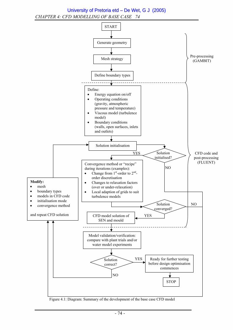
water model. The process followed by the author to obtain a correct solution is

best described in the diagram (Figure 4.1) in the section that follows. The process,

as can be seen in Figure 4.1, involves a number of iterations to individually

change settings in FLUENT and/or model geometry and gridding strategies (in

GAMBIT) until a physically correct and converged solution is obtained.

4.1.3 Summary: approach to base case CFD modelling

Refer to Figure 4.1 for a summary of the approach followed by the author to

obtain a satisfactory CFD solution for the base case.

- 73 -



Figure 4.1: Diagram: Summary of the development of the base case CFD model

NO

Modify: • mesh • boundary types • models in CFD code • initialisation mode • convergence method and repeat CFD solution

NO

NO

YES

YES

YES

CFD code and post-processing

(FLUENT)

Pre-processing (GAMBIT)

STOP

Ready for further testing before design optimisation

commences

Solution correct?

Model validation/verification: compare with plant trials and/or

water model experiments

CFD model solution of SEN and mould

Solution converged?

Convergence method or “recipe” during iterations (examples): • Change from 1st-order to 2nd-

order discretisation • Changes to relaxation factors

(over or under-relaxation) • Local adaption of grids to suit

turbulence models

Solution initialised?

Solution initialisation

Define: • Energy equation on/off • Operating conditions

(gravity, atmospheric pressure and temperature)

• Viscous model (turbulence model)

• Boundary conditions (walls, open surfaces, inlets and outlets)

Define boundary types

Mesh strategy

Generate geometry

START

- 74 -



In the sections that follow, the specific gridding strategies used, choices made for

turbulence models and boundary conditions will be discussed, and the reasons

why they are preferred above other models and options will be stated accordingly.

These choices of turbulence models, strategies, “recipes” and other options, will

be repeated for other arbitrary SEN and mould designs for subsequent design

optimisation exercises.

4.2 Description of base case

4.2.1 SEN description

The base case of this design optimisation exercise is the SEN currently3 used at

Columbus Stainless in Middelburg, South Africa.

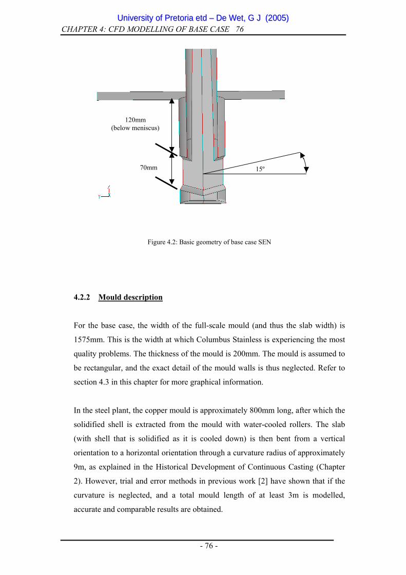
The geometry of the base case SEN is shown in Figure 4.2. The Vesuvius® SEN

has a bifurcated configuration, without a well, and the angle of the SEN ports are

15º upwards from the horizontal. The heights of the SEN ports are 70mm. The

total length of the SEN is approximately 1.1m, and it tapers down from the top

towards the nozzles, simultaneously morphing from a round cross sectional area to

an almost rectangular cross sectional area. The submerged depth of the base case

is 120mm, measured from the top of the nozzle port to the meniscus surface.

However, during continuous casting, the submerged depth is varied from 80mm to

approximately 200mm.

An extract of the drawings for the base case SEN design can be viewed in

Appendix G.4

3 Currently refers to 2001/2002. Another SEN design, which comprises a well-type configuration, is to replace the current type without the well. Refer to Appendix H for the details and drawings. 4 Appendix G: Copyright: Vesuvius, South Africa.

- 75 -



15º

120mm (below meniscus)

70mm

Figure 4.2: Basic geometry of base case SEN

4.2.2 Mould description

For the base case, the width of the full-scale mould (and thus the slab width) is

1575mm. This is the width at which Columbus Stainless is experiencing the most

quality problems. The thickness of the mould is 200mm. The mould is assumed to

be rectangular, and the exact detail of the mould walls is thus neglected. Refer to

section 4.3 in this chapter for more graphical information.

In the steel plant, the copper mould is approximately 800mm long, after which the

solidified shell is extracted from the mould with water-cooled rollers. The slab

(with shell that is solidified as it is cooled down) is then bent from a vertical

orientation to a horizontal orientation through a curvature radius of approximately

9m, as explained in the Historical Development of Continuous Casting (Chapter

2). However, trial and error methods in previous work [2] have shown that if the

curvature is neglected, and a total mould length of at least 3m is modelled,

accurate and comparable results are obtained.

- 76 -



In this dissertation, the CFD modelling and the water model experimental set-up

make use of this assumption, where a total mould length (includes roller-

supported curvature in real steel plants) of 3 m (or more, where possible) is used.

4.2.3 Momentum only vs. momentum and energy combined

In an effort to validate the CFD model with water model experiments, the energy

equation will be neglected, as cold water is used as the fluid in the CFD

modelling. The effect of temperatures on the buoyancy of water is negligible in

any event (the effect on liquid steel flow patterns is deemed to be not that

influential [2]). However, after validation of the CFD model, the modelling fluid

can easily be changed to liquid steel with associated temperature boundary

conditions and energy equation modelling using FLUENT.

4.2.4 Simultaneous SEN and mould modelling

Unlike some other similar CFD work on SEN and moulds [2][3][4][5][6], the

CFD model in this dissertation comprises the simultaneous solution of the SEN

and mould, as the submergence of the SEN into the mould influences the resultant

solution field.

In this dissertation (and optimisation work to follow), the SEN and mould will be

simulated together in one CFD model for better correspondence with plant

circumstances (and the water model). This complicates the flow field, especially

at the nozzle ports as the flow exits into the mould. The importance of mesh

quality at the nozzle exit ports will be discussed in more detail later in section 4.3.

When separating the SEN from the mould, solutions seem to be more stable and

converge quickly to predetermined criteria. However, when evaluating the SEN

- 77 -



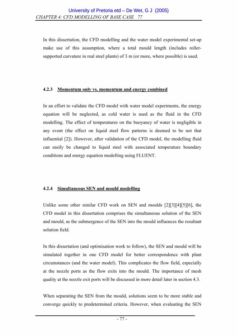
separately, a pressure outlet boundary condition is applied to the SEN where it

exits into the mould cavity. The pressure will typically be assumed to be the

ferrostatic pressure due to the submergence depth of the SEN below the meniscus.

The flow is then solved and the velocity profile of the SEN exit nozzle is applied

as a velocity inlet boundary for the mould in a separate simulation. Refer to Figure

4.3 for the location of the SEN outlet / mould inlet.

However, when measuring (in a SEN and mould combined CFD model after

convergence) the pressure distribution on the SEN port face, a non-constant

pressure distribution is observed. The static and dynamic pressure distributions are

illustrated in Figure 4.4, and show that the pressure distribution is not constant or

a linear pressure distribution. The dynamic pressure distribution in Figure 4.4(b)

includes the effect of the jet kinetic energy (observed as a high total pressure in

the region of high jet velocity). This proves the importance of evaluating the SEN

and mould together in one CFD model, in an effort to capture the real physical

flow situation.

Figure 4.3: Location of SEN outlet port / mould inlet port (quarter model)

SEN outlet / mould inlet

- 78 -



Pascal

0

3 x 103

6 x 103

(a) Static Pascal

-1.2 x 103

0

1.5 x 103

Figure 4.4: Static and Dynamic pressure distribution in 3D SEN port face (quarter model) in Pascal

(b) Dynamic

4.2.5 2D and 3D modelling

Although 3D CFD modelling will be much more representative of the physical

flow situation in the SEN and mould, 2D models are also developed alongside the

3D models. The main reason is the fact that 3D CFD models are much more

computationally expensive than 2D models. If the 2D CFD model solutions are

similar to that of 3D (and there are many similarities – refer to section 4.4.2), it

would be much more sensible to perform design optimisation with 2D models.

Thus, throughout this dissertation, there will be made use of both 2D and 3D CFD

models and, when compared, differences will be pointed out and explained.

- 79 -



4.3 CFD set-up

4.3.1 Geometry and gridding strategy (pre-processing)

Symmetry assumed:

In this dissertation, the flow is assumed to be symmetrical. A half model is

therefore used for the 2D model, and a quarter model for the 3D model. However,

due to small flow differences experienced in continuous casting plants and the

water model, the flow will never be completely symmetrical in practice. The water

model results proved this fact (refer to Chapter 3, section 3.3 where the

asymmetrical flow field is shown in Figure 3.12). The overall geometry (flow

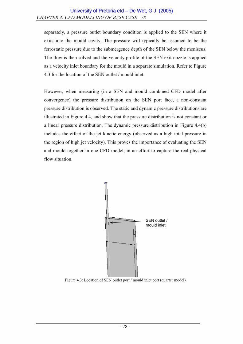
area) can be seen in Figure 4.5, where the 3D quarter model is shown without the

mesh to indicate boundary conditions.

Importance of element types:

Trial and error methods have proven that the element types chosen have a

significant effect on the solution: not only the end result, but also the manner

(stability, numerical errors amongst others) in which the solution approaches

convergence.

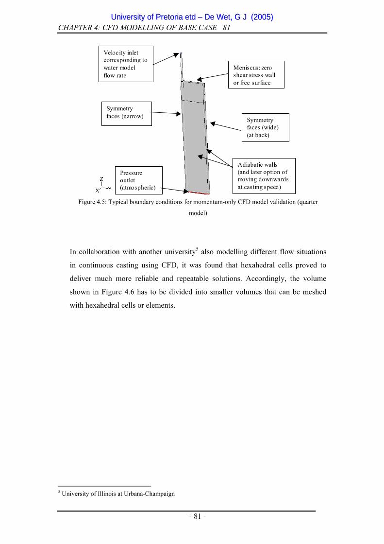
Initially, in order to accommodate later optimisation parameterisation, the volume

around the nozzle area was meshed using an unstructured grid (tetrahedral

elements or volumes). The author used this method as the mentioned volume

(refer to Figure 4.6) will change if the typical nozzle parameters (port height, port

angle for example) change, and unstructured (tetrahedral) grids are automatically

generated by the pre-processor GAMBIT for rather complicated volumes.

However, the most complex flow is found at the SEN nozzles, where the jets exit

into the mould cavity. Subsequently, incorrect flow patterns regularly (but not

always) were observed using unstructured grids at the critical and unstable jet

orifices.

- 80 -



Meniscus: zero shear stress wall or free surface

Symmetry faces (wide) (at back)

Pressure outlet (atmospheric)

Symmetry faces (narrow)

Velocity inlet corresponding towater model flow rate

Adiabatic walls (and later option of moving downwards at casting speed)

Figure 4.5: Typical boundary conditions for momentum-only CFD model validation (quarter

model)

In collaboration with another university5 also modelling different flow situations

in continuous casting using CFD, it was found that hexahedral cells proved to

deliver much more reliable and repeatable solutions. Accordingly, the volume

shown in Figure 4.6 has to be divided into smaller volumes that can be meshed

with hexahedral cells or elements.

- 81 -

5 University of Illinois at Urbana-Champaign



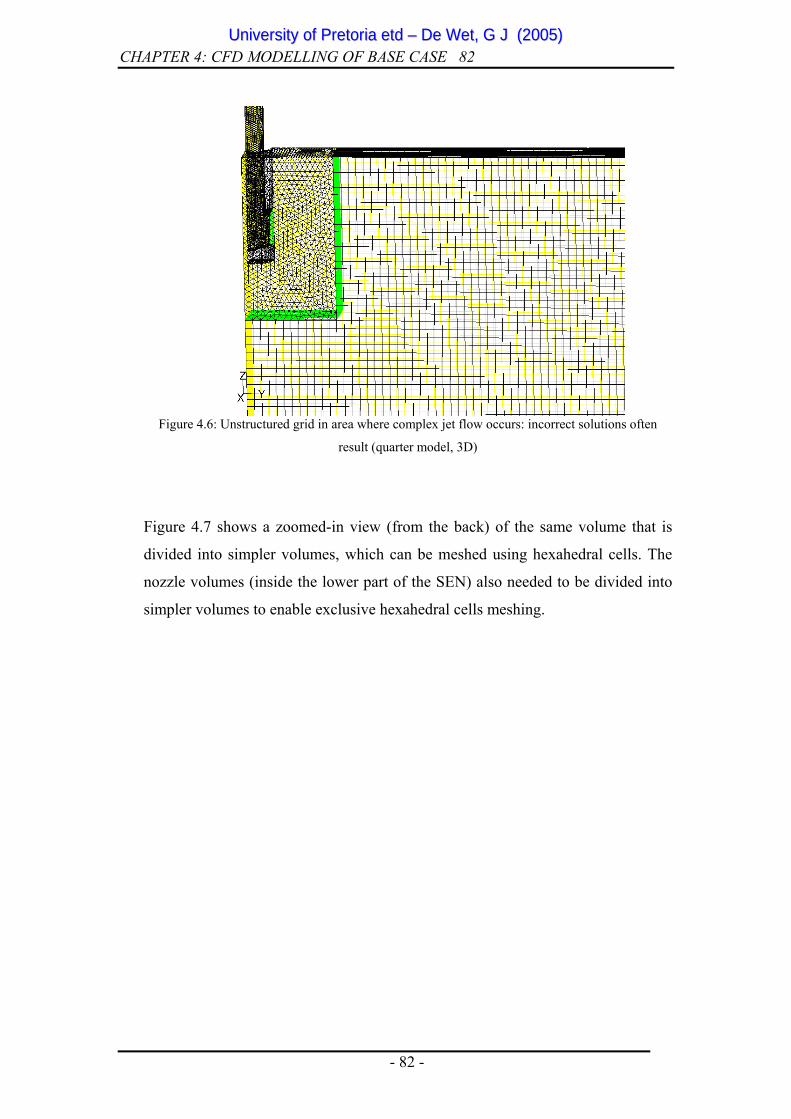
Figure 4.6: Unstructured grid in area where complex jet flow occurs: incorrect solutions often

result (quarter model, 3D)

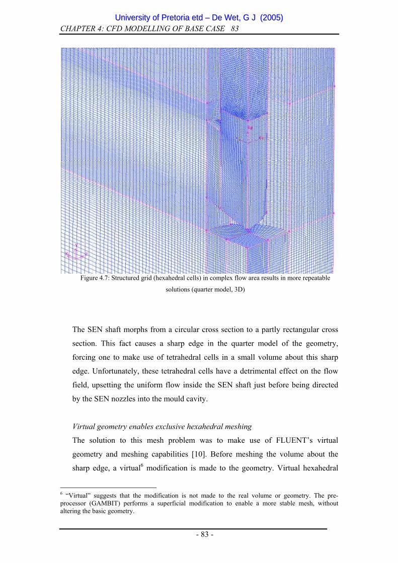
Figure 4.7 shows a zoomed-in view (from the back) of the same volume that is

divided into simpler volumes, which can be meshed using hexahedral cells. The

nozzle volumes (inside the lower part of the SEN) also needed to be divided into

simpler volumes to enable exclusive hexahedral cells meshing.

- 82 -



Figure 4.7: Structured grid (hexahedral cells) in complex flow area results in more repeatable

solutions (quarter model, 3D)

The SEN shaft morphs from a circular cross section to a partly rectangular cross

section. This fact causes a sharp edge in the quarter model of the geometry,

forcing one to make use of tetrahedral cells in a small volume about this sharp

edge. Unfortunately, these tetrahedral cells have a detrimental effect on the flow

field, upsetting the uniform flow inside the SEN shaft just before being directed

by the SEN nozzles into the mould cavity.

Virtual geometry enables exclusive hexahedral meshing

The solution to this mesh problem was to make use of FLUENT’s virtual

geometry and meshing capabilities [10]. Before meshing the volume about the

sharp edge, a virtual6 modification is made to the geometry. Virtual hexahedral

6 “Virtual” suggests that the modification is not made to the real volume or geometry. The pre-processor (GAMBIT) performs a superficial modification to enable a more stable mesh, without altering the basic geometry.

- 83 -



cells are then generated within the virtual geometry. Subsequently, the entire 3D

model of the SEN and mould can be meshed with the exclusive use of hexahedral

cells, which, as trial and error has proven, is essential for correct and repeatable

CFD results.

The use of virtual volumes and virtual hexahedral cells was also incorporated in

the GAMBIT script file (for automatic geometry and mesh generation) in Chapter

5, during the design space exploration as an optimisation exercise to find an

optimum 3D SEN design.

Similar problems also occurred in 2D modelling: subsequently quadrilateral

elements are used instead of unstructured pave elements. This was achieved by

dividing all areas with 5 or more sides (polygons) into quadrilateral areas or cells,

before attempting to mesh the geometry.

4.3.2 Boundary conditions

The typical boundary conditions specified in the CFD model for the base case are

shown in Figure 4.5 above. The 2D boundary conditions are similar to that of the

3D model.

Meniscus boundary condition:

The meniscus boundary condition (see Figure 4.5 above) can either be a zero

shear stress wall, or a free surface with a volume air generated above the latter.

Using the Volume of Flow (VOF) method in FLUENT, the behaviour of the free

surface (meniscus) and the influence on the flow solution inside the mould was

evaluated. The VOF-method required very expensive unsteady solvers: thus only

a 2D simulation was evaluated. The mould flow fields compared favourably (refer

to Appendix I); consequently the less expensive boundary condition (zero shear

stress wall or slip wall which simulates a free surface) will be used for later

optimisation studies and for the base case CFD model validations in this chapter.

Moreover, it is currently much easier to extract heat from the meniscus by simply

- 84 -



specifying a heat flux boundary condition. However, in possible future work when

the exact behaviour of the meniscus becomes important, the use of the VOF-

method (or something similar) will be a necessity.

Velocity inlet:

The velocity inlet, specified as perpendicular to the inlet boundary, corresponds to

the water model flow rate. Later, it can easily be correlated with the steel mass

flow rate taking into account the density of the steel to be cast. The stopper of the

tundish (which is also modelled in the water model – refer to Chapter 3), which

controls the flow to the mould, is taken into account in the CFD model by

modelling the inlet boundary as an annular inlet.

Symmetry faces:

The assumption of symmetry in the width and thickness of the mould allows one

to only model a quarter of the SEN and mould (3D model). The solution is thus

assumed to be identical in all four quarters. By defining two symmetry planes,

FLUENT can solve the entire mould model – by only solving a quarter model.

Mould walls:

Adiabatic walls (only for model verification purposes):

For the purpose of the base case CFD model validation, the walls will be

considered to be adiabatic and stationary. However, the model can easily be

altered to move the walls at casting speed and with a liquidus temperature

imposed, to more closely simulate plant conditions for later optimisation

evaluations.

Walls at liquidus temperature: (for model of steel plant):

As soon as the CFD model of the base case is verified using the water model

results, it is easy to alter the boundary conditions of the walls in FLUENT. The

boundary conditions on the mould walls will include the following settings:

• walls at liquidus temperature (1450 ºC)

• walls moving downwards at casting speed (1.0 m/min for base case)

- 85 -



• heat flux from the flow field in the copper mould contact area and from

meniscus (approximately 300 000W/m2, which must be converted for 2D

models)

Owing to the fact that only thick slab casting is considered in this work, it is

assumed that the shape of the solidifying shell does not influence the fluid flow, as

the walls are assumed to be straight. However, the author is aware that shell

forming may have a profound influence on the flow patterns with thin slab

casting, which is beyond the scope of this work.

Subsequently, only single-phase flow will be evaluated in the mould volume, as it

is assumed that solidification does not take place.

Pressure outlet (atmospheric):

Trial and error methods have proven that the use of an atmospheric pressure outlet

results in more physically correct solutions, than using an outflow (zero gradient)

outlet. As the steel solidifies in the strand, the correct choice of boundary

conditions is difficult. Rather, this boundary location is chosen to be far enough

away, in such a way not to influence the flow patterns around the SEN. At first, a

mould length of 3m was used and deemed to be far enough away; however, with

later 3D design exploration models (refer to Chapter 5, section 5.6), a mould or

rather strand length of 4.3m was used, with much success7.

4.3.3 CFD options and assumptions

Steady-state:

The steady-state solution for the CFD flow field is required in order to compare

with the water model – it is assumed that the water model has reached a steady

flow field as soon as the meniscus level is stable (when the dye is injected – refer

to Chapter 3 for more information).

7 Solutions were more stable and converged faster due to lack of excessive backflow through the mould exit.

- 86 -



However, some SEN designs caused a very unstable simulated flow field, where

the jets never really stabilised, but rather fluctuated around an average jet position.

This unsteady behaviour was mostly noticed on 3D CFD models with wide widths

(1575mm), and thus did not severely influence the optimisation studies in Chapter

5. Some recommendations for future work concerning unsteady flow fields are

discussed in Chapter 6.

Operating conditions:

Operating conditions include specifying the

• atmospheric pressure (which can of course be lower than 101.3 kPa

depending on height above sea level);

• surrounding atmospheric temperature; and the

• gravity vectors (depending on orientation of model).

Turbulence model:

A jet exiting into a larger cavity (such as the SEN nozzle exiting into the mould)

definitely suggests turbulent flow [9]. FLUENT offers a number of viscous and

turbulence models to suit most flow problem types. Whenever a turbulent flow

situation is anticipated, the k-ε turbulence model is usually implemented because

of its adequate accuracy (in most circumstances) as opposed to relative little

computing time.

Whenever more accurate turbulent models are implemented, such as Large Eddy

Simulation (LES) or the Reynolds Stress Model (RSM), a considerable increase in

computing time is required. With LES, an extremely fine mesh is necessary to

successfully use this sub-grid scale turbulence model [38]. With RSM, on the

other hand, 7 equations must be solved for each cell every iteration for 3D (as

opposed to the k-ε model’s 2 equations).

FLUENT compares the relevant turbulence models as follows (Table 4.1):

- 87 -



Table 4.1: Comparison between different turbulence models [10] Model Strengths Weaknesses

Standard k-ε Robust, economical, reasonably

accurate; long accumulated

performance data

Mediocre results for complex

flows involving severe pressure

gradients, strong streamline

curvature, swirl and rotation

RNG8 k-ε Good for moderately complex

behaviour like jet impingement,

separating flows, swirling flows,

and secondary flows

Subjected to limitations due to

isotropic eddy viscosity

assumption

Realisable k-ε Offers largely the same benefits

as RNG; resolves round jet

anomaly however



assumption

Reynolds Stress Model (RSM) Physically most complete model

of large and small-scale

turbulence (history, transport,

and anisotropy of turbulent

stresses all accounted for);

isotropy not assumed

Requires more CPU effort (2 to 3

times more than k-ε methods);

tightly coupled momentum and

turbulence equations

Standard k-ω9 Apart from similar strengths as

Standard k-ε model, it

incorporates low Re-number

effects and shear flow spreading.

Applicable to wall-bounded

flows and free shear flows.



assumption. Also marginally

more expensive due to more

built-in models and

sophistication for specific flow

circumstances.

SST k-ω Blend robust and accurate

formulation of k-ω model in

near-wall regions with free

stream independence of k-ε in far

field. More accurate and reliable

for wider class of flows, i.e.,

adverse pressure gradient flows

(e.g., airfoils), transonic

shockwaves, etc.



assumption

Large Eddy Simulation (LES) Models small-scale turbulence

directly; no assumptions on flow

Requires extremely fine mesh

and (mostly) exclusive hexagonal

8 RNG: Renormalisation Group Method. This k-ε method encompasses the standard k-ε equations, with the addition of applying a rigorous statistical technique [10]. 9 Addition to turbulence models available in FLUENT since 2003

- 88 -



conditions (structured) grids. Subsequently

ridiculously computationally

expensive and not suited for

optimisation work.

Trial and error methods proved that the choice of a turbulence model has a radical

effect on this particular flow field. The flow field is sensitive to the combination of

turbulence model, mesh quality and solution procedure followed. For this dissertation,

the RSM model was selected for some 3D simulations owing to its better grid

independence (as opposed to the k-ε model). The RSM model is further more accurate

in predicting real turbulent 3D flow fields, as turbulent velocity fluctuations around a

time-averaged mean velocity is computed by solving transport equations for each of

the terms in the Reynolds stress tensor [10]. The family of k-ε and k-ω models assume

turbulent fluctuations to be the same in all directions (isotropic turbulence – also see

Table 4.1). The anisotropic nature of turbulence in highly swirling flows and stress-

driven secondary flows has a dominant effect on the mean flow situation – therefore

RSM is clearly the superior model for the SEN and mould model [10].

The cost of RSM however disqualified it for use in an optimisation environment,

where many simulations need to be performed. The base case SEN design (with a

submergence depth of 200mm, however) was modelled using the RSM turbulence

model. The mesh consisted of approximately 3 million cells. In order to ensure

convergence, the CFD model iterated for several months on a 3 GHz Intel Pentium 4,

reaching approximately 44 000 iterations. This proves that the RSM turbulence model

is not suitable for general optimisation use with current computational power.

However, since the addition of the k-ω turbulence model to FLUENT in 2003 [10],

this much less expensive 2-equation model proved to be well suited for jet-like flows.

The Standard k-ω model is based on the Wilcox k-ω model [50]. Both k-ω turbulence

models (Standard (STD) and Shear Stress Transport (SST)) [51] incorporate

modifications for low Re-number effects, compressibility, and shear flow spreading.

Wilcox’s model predicts shear flow spreading rates that are in close agreement with

- 89 -


CHAPTER 4: CFD MODELLING OF BASE CASE 90 measurements for far wakes, mixing layers, as well as plane, round and radial jets.

These models are thus applicable to wall-bounded flows and free shear flows.

The Standard k-ω model proved to be most suited for 3D CFD models of the SEN and

mould. This turbulence model was also used successfully in Chapter 5, section 5.6,

during a design space exploration optimisation exercise for specifically 3D SEN and

mould models.

On the other hand, 2D modelling proved to be accurate with the k-ε Realisable model

[39]. Although this model also assumes isotropic turbulence, the effect on the mean

flow is negligible in 2D modelling. The k-ε Realisable model (as opposed to the

Standard k-ε model) is more suited for flow features that include strong streamline

curvature, vortices, rotation and complex secondary flow features (see Table 4.1).

Near-wall treatments:

Most k-ε, k-ω, and RSM turbulence models will not predict correct near-wall

behaviour if integrated down to the wall. For this reason, so-called wall functions

need to be used in conjunction with these turbulence models to empirically predict the

correct transition from the fully turbulent region to the laminar viscous sub layer.

FLUENT compares three near-wall treatments to be used in conjunction with any of

the turbulence models discussed above (Table 4.2):

Table 4.2: Comparison between different near-wall treatments [10]

Wall functions Strengths Weaknesses

Standard wall functions Robust, economical, reasonably

accurate

Empirically based on simple high

Re-number flows;

poor for low Re-number effects,

p∇ , strong body forces, highly

3D flows

Non-equilibrium wall functions Accounts for p∇ effects, allows

non-equilibrium for:

separation, re-attachment and

impingement

Poor for low Re-number effects,

massive transpiration, severe

p∇ , strong body forces, highly

3D flows

- 90 -


CHAPTER 4: CFD MODELLING OF BASE CASE 91 Wall functions Strengths Weaknesses

Two-layer zonal model Does not rely on law-of-the-wall,

good for complex flows,

especially applicable to low Re-

number flows

Requires finer mesh resolution

and therefore larger CPU and

memory resources

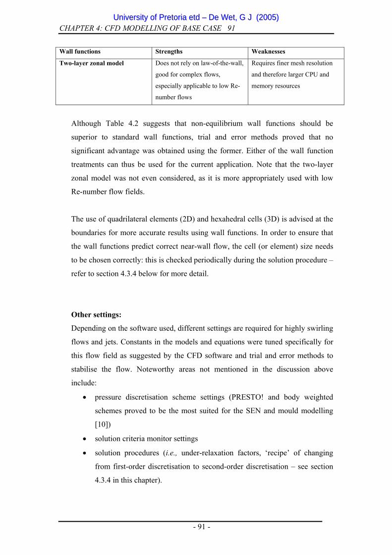
Although Table 4.2 suggests that non-equilibrium wall functions should be

superior to standard wall functions, trial and error methods proved that no

significant advantage was obtained using the former. Either of the wall function

treatments can thus be used for the current application. Note that the two-layer

zonal model was not even considered, as it is more appropriately used with low

Re-number flow fields.

The use of quadrilateral elements (2D) and hexahedral cells (3D) is advised at the

boundaries for more accurate results using wall functions. In order to ensure that

the wall functions predict correct near-wall flow, the cell (or element) size needs

to be chosen correctly: this is checked periodically during the solution procedure –

refer to section 4.3.4 below for more detail.

Other settings:

Depending on the software used, different settings are required for highly swirling

flows and jets. Constants in the models and equations were tuned specifically for

this flow field as suggested by the CFD software and trial and error methods to

stabilise the flow. Noteworthy areas not mentioned in the discussion above

include:

• pressure discretisation scheme settings (PRESTO! and body weighted

schemes proved to be the most suited for the SEN and mould modelling

[10])

• solution criteria monitor settings

• solution procedures (i.e., under-relaxation factors, ‘recipe’ of changing

from first-order discretisation to second-order discretisation – see section

4.3.4 in this chapter).

- 91 -



4.3.4 Solution Procedure

Initialisation:

During the iteration process, certain milestones must be reached before switching

to more accurate solver algorithms. For example, before the iteration process can

commence, an initial solution must be guessed. This initial estimate of a flow field

can thus be seen as a first milestone before the iteration process can begin.

1st-order and 2nd-order discretisation schemes:

Due to the nature of the numerical solution of the discretised Navier-Stokes

equations, the solution needs to “propagate” from the inlet boundary through the

SEN into the mould cavity. In order to speed up this process, the first few hundred

iterations (may differ immensely depending on type of grid, 2D or 3D, type of

turbulence model, etc.) are performed with first-order discretisation.

As the first-order solution approaches convergence, the second-order

discretisation scheme is enabled, using the solution of the first-order scheme as an

initial solution from which to iterate. When the second-order solution has

converged, it is assumed to be the solution to the initial CFD problem.

Under- and over-relaxation factors:

As explained in the Literature Survey (Chapter 2, section 2.3.4.2), it is often

necessary to adjust the over-relaxation factors to prevent the non-linear Navier-

Stokes equations from diverging. Under-relaxation comprises the slowing down of

changes from iteration to iteration. Over-relaxation (accelerating these changes) is

often used to test whether a “converged” solution is indeed converged and stable.

However, trial and error methods have indicated that a certain ‘recipe’ or rather

procedure is required to ensure convergence of SEN and mould CFD problems. It

is necessary to adjust the under-relaxation factors every few hundred iterations

(see below for solution procedure and Figure 4.8) to ensure that the residuals

converge sufficiently. As soon as the solution seems to be nearing convergence

(also comparing real flow indicators monitored during the iteration procedure), the

- 92 -



relaxation factors can be adjusted upwards (towards over-relaxation) to ensure a

true converged solution.

Wall functions – grid adaption necessary:

In order for the wall functions (described in section 4.3.3) to predict the near-wall

flow correctly, the grid cells adjacent to the wall need to be sized correctly. The

size is determined by the y+-value of that cell: the y+-value of a cell is a function

of the velocity of and the properties (density, viscosity inter alia) of the fluid in

that cell, and is in fact a local Reynolds number based on the friction velocity and

the normal spacing of the first cell. For the k-ε and k-ω turbulence models, the

wall function approach requires the y+-value to be between 50 and 500

[dimensionless].

Whenever reverse flow is experienced over any boundaries in a CFD model, the

situation may arise that mass imbalances occur. The SEN and mould CFD model

is an example where mass imbalances occur: due to a recirculation zone in the

mould, reverse flow is experienced over the pressure outlet boundary. These mass

imbalances must be periodically rectified during the solution procedure using grid

adaption (refer to the solution procedure below).

Grid adaption and virtual meshes:

Whenever virtual meshes are required and used (for 3D mesh of SEN and mould),

normal grid adaption during solution iterations is not possible. Consequently, grid

adaption due to mass-imbalances is also not possible.

Dynamic grid adaption:

However, a new feature added to FLUENT (FLUENT 6.1.1. [10]) enables the user

to dynamically adapt the virtual grid during the solution procedure. Starting (since

initialisation) from an initial mesh size (typically 500 000 cells for this 3D case),

the mesh is refined and coarsened as the solution proceeds, based on velocity

gradients (other criteria can also be used). This is an attempt to follow the

formation of the SEN jet with grid clustering. A maximum cell count of

approximately 850 000 is reached in this process depending on the complexity of

- 93 -



the flow field and the SEN geometry used (part size, number of design

parameters, etc.). The dynamic mesh adaption option is chosen and configured

before the solution iteration process is started, and dynamically adapts the mesh as

the solution proceeds until sufficient convergence is achieved.

Other solution procedure settings:

Different functions and schemes can be switched on and off during the solution

procedure to aid the solution to meet the convergence criteria as soon as possible.

Obviously, these setting changes can only be performed when the iteration

procedure has been interrupted. Over-zealous interruptions and setting changes

can have a negative impact on the convergence and subsequent correctness of the

CFD solution.

The (typical) solution procedure used to obtain the results displayed in section 4.4

is shown below. Refer to Figure 4.8 for the graphical presentation of the solution

procedure, using the residuals.

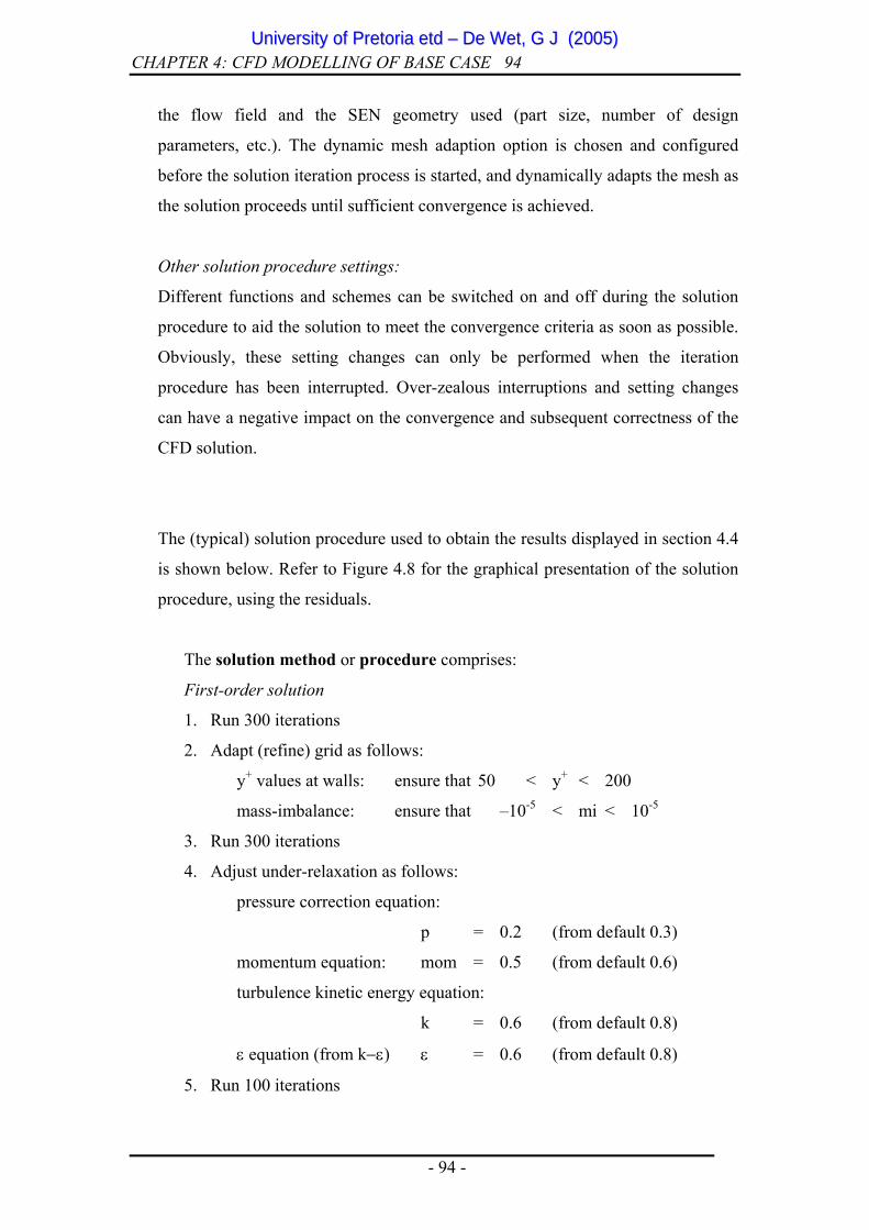
The solution method or procedure comprises:

First-order solution

1. Run 300 iterations

2. Adapt (refine) grid as follows:

y+ values at walls: ensure that 50 < y+ < 200

mass-imbalance: ensure that –10-5 < mi < 10-5


4. Adjust under-relaxation as follows:

pressure correction equation:

p = 0.2 (from default 0.3)

momentum equation: mom = 0.5 (from default 0.6)

turbulence kinetic energy equation:

k = 0.6 (from default 0.8)

ε equation (from k−ε) ε = 0.6 (from default 0.8)


- 94 -



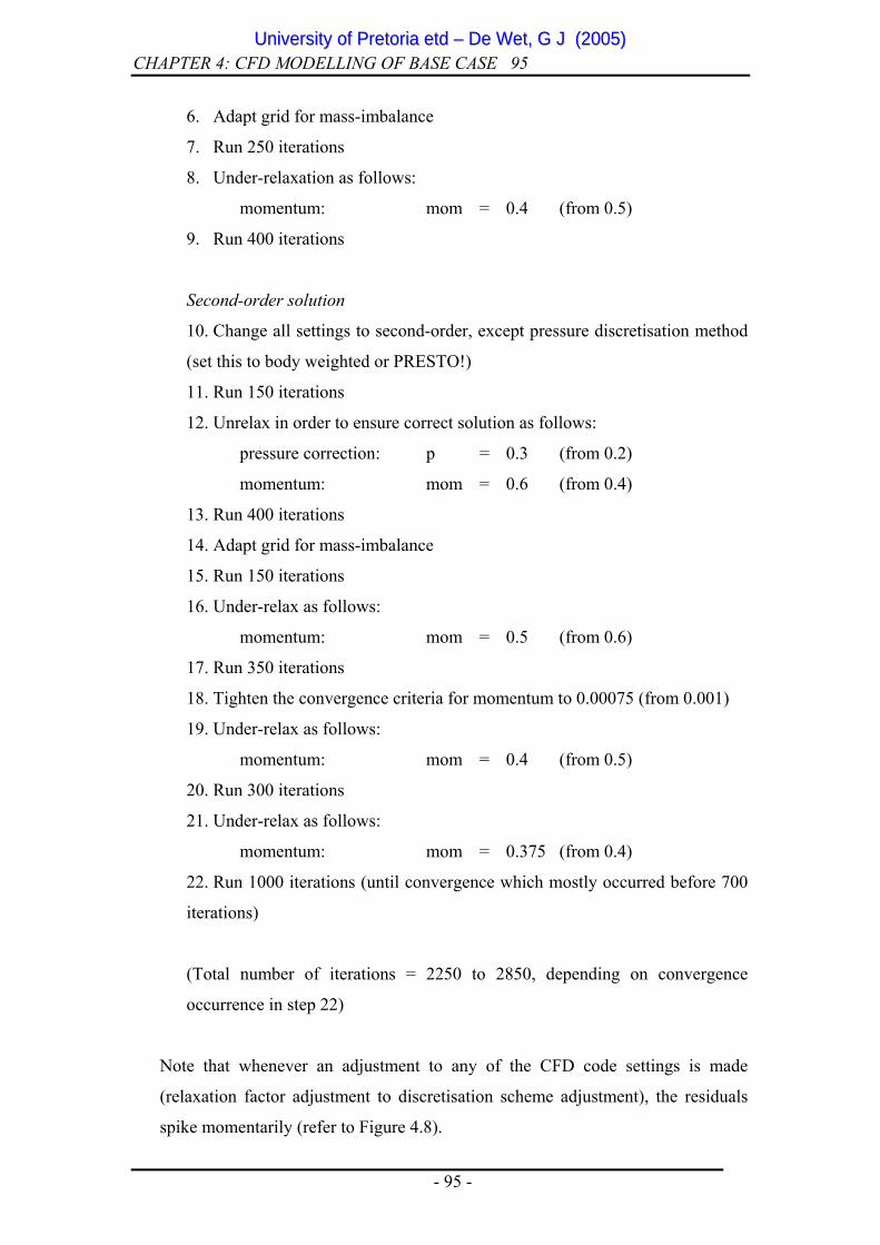
6. Adapt grid for mass-imbalance


8. Under-relaxation as follows:

momentum: mom = 0.4 (from 0.5)


Second-order solution

10. Change all settings to second-order, except pressure discretisation method

(set this to body weighted or PRESTO!)


12. Unrelax in order to ensure correct solution as follows:

pressure correction: p = 0.3 (from 0.2)



14. Adapt grid for mass-imbalance


16. Under-relax as follows:



18. Tighten the convergence criteria for momentum to 0.00075 (from 0.001)






22. Run 1000 iterations (until convergence which mostly occurred before 700

iterations)

(Total number of iterations = 2250 to 2850, depending on convergence

occurrence in step 22)

Note that whenever an adjustment to any of the CFD code settings is made

(relaxation factor adjustment to discretisation scheme adjustment), the residuals

spike momentarily (refer to Figure 4.8).

- 95 -



Figure 4.8: Residuals during solution procedure (‘recipe’)

4.4 CFD model: Verification Results

4.4.1 CFD model verification: mimic water model

The reason as to why a water model was designed and built by the University of

Pretoria (the author) was to validate the CFD model of the SEN and mould before

any design optimisation is attempted.

The first step to validate the model is to concentrate on the flow patterns only

(momentum only), by exactly imitating the 40%-scaled water model. If the CFD

momentum model closely matches the flow patterns of the 40%-scaled water

model, the model10 can be assumed to be acceptable.

From here, it is rather a straightforward exercise to extend the model to imitate

real plant circumstances, by scaling the geometry to full-scale, enabling the

10 The CFD “model” includes all aspects covered in Figure 4.1, and briefly includes geometry and gridding strategy, flow assumptions, CFD options and CFD assumptions, boundary conditions, and finally the solution procedure.

- 96 -



energy equation (and therefore allow temperature and buoyancy effects), and

adjusting and supplementing the boundary conditions. Refer to section 4.5 for

these actions. It should however be stressed that a high-fidelity modelling of the

plant situation (e.g., modelling of mould oscillation, solidification,

conglomeration of inclusions, etc.) falls outside the scope of this dissertation.

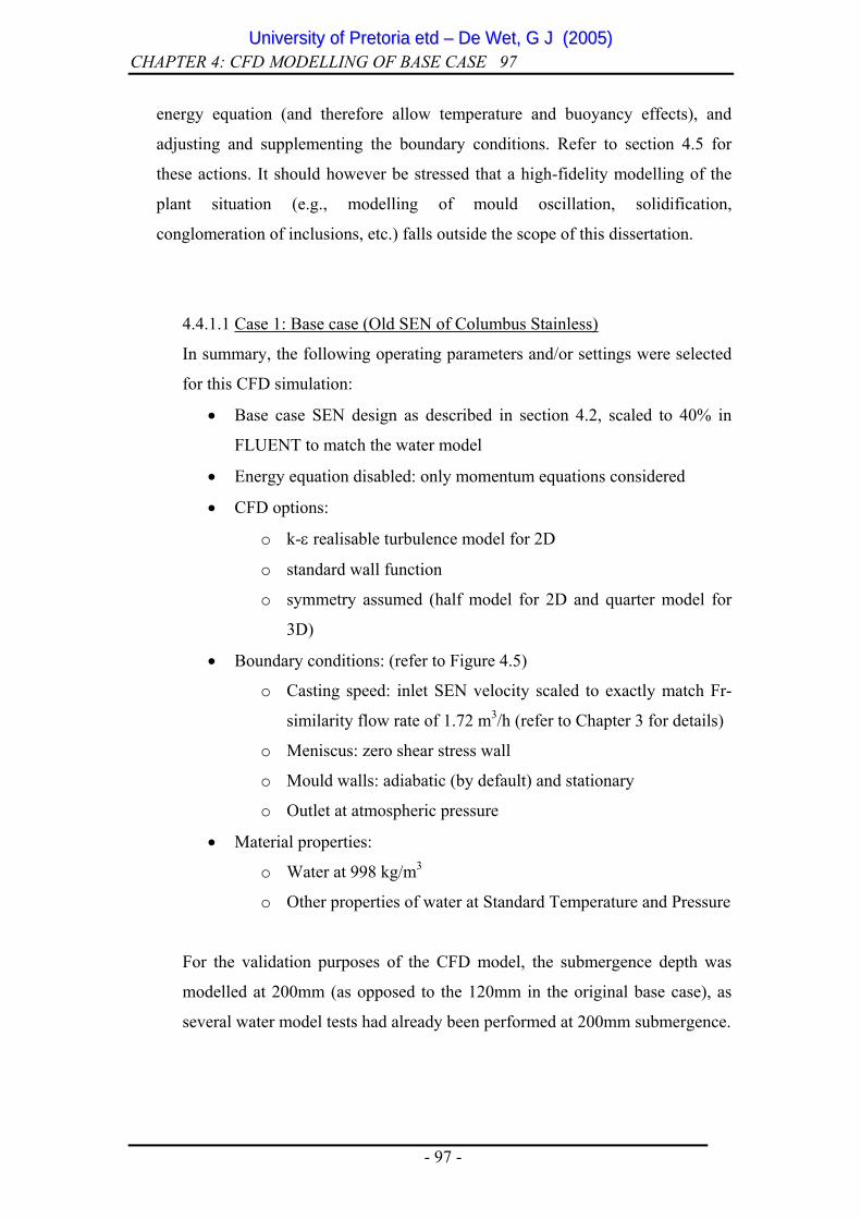
4.4.1.1 Case 1: Base case (Old SEN of Columbus Stainless)

In summary, the following operating parameters and/or settings were selected

for this CFD simulation:

• Base case SEN design as described in section 4.2, scaled to 40% in

FLUENT to match the water model

• Energy equation disabled: only momentum equations considered

• CFD options:

o k-ε realisable turbulence model for 2D

o standard wall function

o symmetry assumed (half model for 2D and quarter model for

3D)

• Boundary conditions: (refer to Figure 4.5)

o Casting speed: inlet SEN velocity scaled to exactly match Fr-

similarity flow rate of 1.72 m3/h (refer to Chapter 3 for details)

o Meniscus: zero shear stress wall

o Mould walls: adiabatic (by default) and stationary

o Outlet at atmospheric pressure

• Material properties:

o Water at 998 kg/m3

o Other properties of water at Standard Temperature and Pressure

For the validation purposes of the CFD model, the submergence depth was

modelled at 200mm (as opposed to the 120mm in the original base case), as

several water model tests had already been performed at 200mm submergence.

- 97 -



Refer to Table 4.3 for the comparison of the 2D CFD model with the water

model results. For the sake of completeness, the 2D results (Table 4.3) where

the meniscus boundary was evaluated as a free surface (as opposed to a less

expensive slip wall) are also shown to demonstrate the favourable comparison

(also see Appendix I).

It can be seen that the 2D CFD model predicts a jet that penetrates deeper than

observed in the water model. The intensity of the 2D simulated jet seems to be

higher than that of the water model, i.e., higher velocities are concentrated on

the centreline of the simulated jet, as opposed to the more dissipated nature of

the water model jet. The same trend is also observed when comparing

simulated 2D and 3D results, with the 3D results being more representative of

the water model observations.

The CFD results in Table 4.3 are displayed in the form of contours of velocity

magnitude, just to highlight the flow pattern (momentum only) for validation

purposes.

Table 4.3: Verification of 2D CFD model (slip wall and free surface meniscus boundary

condition) with 40%-scaled water model. CFD results displayed using contours of velocity

magnitude

CFD Scale

2D: zero shear stress (slip) wall meniscus

UP 40% Water model 2D: free surface meniscus

1

0.5

0

m/s

Slip wall Slip wall

Free surface Free surface

air

Base case (Old SEN): Submergence 80mm (200mm full-scale); Fr-similarity 1.72m3/h

- 98 -



4.4.1.2 Case 2: New SEN of Columbus Stainless

Columbus Stainless also requested water model testing of their more recent

SEN design. Subsequently, the author was in possession of another case

(physical SEN insert for the water model experimental set-up) to verify the

CFD model of the SEN and mould.

The parameters and/or settings were identical to that of the base case (Old

SEN), except for the different SEN design. The new design has the following

parameters: (refer to Appendix H for drawings of new SEN design)

• port angle: 15º upward

• port height: 60 mm

• port width and radii: 45mm and 35mm (similar to base case design)

• well depth: 15mm

• well angle: flat

Refer to Table 4.4 (below) for the comparison of the 2D CFD model of the

New SEN with the 40%-scaled water model results.

- 99 -



Table 4.4: Verification of 2D CFD model (slip wall and free surface meniscus boundary

condition) with 40%-scaled water model. CFD results displayed using contours of velocity

magnitude CFD Scale

2D: zero shear stress (slip) wall meniscus

UP 40% Water model 2D: free surface meniscus

1

0.5

0

m/s

Slip wall

Free surface Free surface

air

New SEN: Submergence 80mm (200mm full-scale); Fr-similarity 1.72m3/h

Again, it can be seen that the 2D CFD model predicts a jet that penetrates

deeper than that observed in the water model. The line drawn inside the jet (all

three figures in Table 4.4) corresponds closely to the concentrated jet of the

2D CFD solutions, indicating the more dissipative jet of the water model.

4.4.2 2D vs. 3D verification results

4.4.2.1 3D verification results

Settings:

Apart from extending the 2D CFD model settings and parameters to 3

dimensions, the turbulence model choice had to be altered:

As trial and error methods have proven, the k-ε turbulence models are not

suited for 3D modelling. Consequently, as explained in section 4.3.3, the

rather expensive RSM turbulence model was selected for this validation

study. However, it was soon realised that the RSM turbulence model is too

- 100 -



computational expensive for general optimisation purposes, as it also

demands a fine mesh (in excess of 2 million cells), apart from the fact that

it requires 7 equations to be solved per iteration (as opposed to only 2 of

the k-ε models). The result displayed in Table 4.5 has run for 52000

iterations, taking several months on a 3GHz Pentium IV with 2GB RAM

computer to complete.

The less expensive Standard k-ω turbulence model (also only 2 equations

per iteration) was selected as the turbulence model for the 3D model of the

steel plant (section 4.5), which proved to be a good assumption, especially

for smaller width moulds.

Refer to the Table 4.5 for the comparison between the 3D models of both

turbulence models (k-ω and RSM) on the base case SEN design, and the 40%-

scaled water model. The contours of velocity magnitude on the symmetry

plane (i.e., centre plane of the mould) of the CFD models are displayed. Note

that both CFD models were configured to exactly imitate the 40%-scaled

water model test.

Note on Table 4.5: differences between 3D CFD models and water model

results

There is a noticeable difference between the 3D CFD models (k-ω and RSM

turbulence closure) and the 40%-scaled water model. As more experience in

SEN 3D modelling was gained during this study, it was noticed that the wider

widths presented problems for most CFD methods. For example, the residuals

struggled to fall below 3rd-order convergence. Moreover, the flow field seem

unstable and pseudo-transient, although otherwise suggested by water model

experiments. Furthermore, the pseudo-transient nature of the results seems to

worsen as soon as 2nd-order upwinding is introduced.

Nevertheless, later 3D optimisation work in Chapter 5 was conducted on

narrower slab widths (range 1000 – 1300mm), and the 3D CFD models

- 101 -



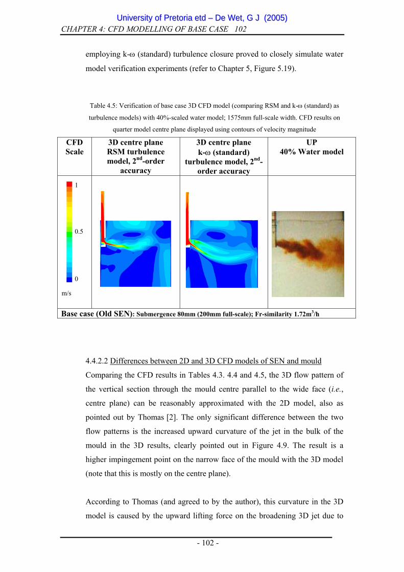
employing k-ω (standard) turbulence closure proved to closely simulate water

model verification experiments (refer to Chapter 5, Figure 5.19).

Table 4.5: Verification of base case 3D CFD model (comparing RSM and k-ω (standard) as

turbulence models) with 40%-scaled water model; 1575mm full-scale width. CFD results on

quarter model centre plane displayed using contours of velocity magnitude

CFD Scale

3D centre plane RSM turbulence model, 2nd-order

accuracy

3D centre plane k-ω (standard)

turbulence model, 2nd-order accuracy

UP 40% Water model

1

0.5

0

m/s

Base case (Old SEN): Submergence 80mm (200mm full-scale); Fr-similarity 1.72m3/h

4.4.2.2 Differences between 2D and 3D CFD models of SEN and mould

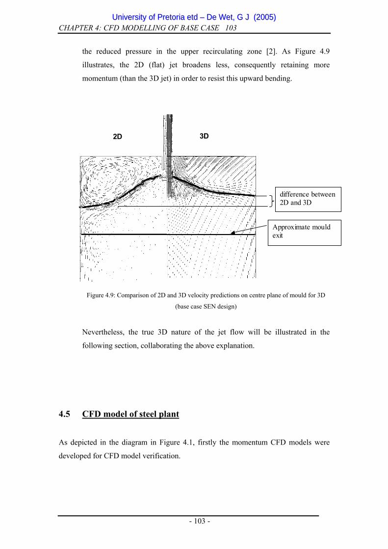
Comparing the CFD results in Tables 4.3. 4.4 and 4.5, the 3D flow pattern of

the vertical section through the mould centre parallel to the wide face (i.e.,

centre plane) can be reasonably approximated with the 2D model, also as

pointed out by Thomas [2]. The only significant difference between the two

flow patterns is the increased upward curvature of the jet in the bulk of the

mould in the 3D results, clearly pointed out in Figure 4.9. The result is a

higher impingement point on the narrow face of the mould with the 3D model

(note that this is mostly on the centre plane).

According to Thomas (and agreed to by the author), this curvature in the 3D

model is caused by the upward lifting force on the broadening 3D jet due to

- 102 -



the reduced pressure in the upper recirculating zone [2]. As Figure 4.9

illustrates, the 2D (flat) jet broadens less, consequently retaining more

momentum (than the 3D jet) in order to resist this upward bending.

Figure 4.9: Comparison of 2D and 3D velocity predictions on centre plane of mould for 3D

Nevertheless, the true 3D nature of the jet flow will be illustrated in the

.5 CFD model of steel plant

2D 3D

Approximate mould exit

difference between 2D and 3D

(base case SEN design)

following section, collaborating the above explanation.

4

s depicted in the diagram in Figure 4.1, firstly the momentum CFD models were

A

developed for CFD model verification.

- 103 -


CHAPTER 4: CFD MODELLING OF BASE CASE 104 The next step, now that the author is quite confident in the accuracy of the CFD

modelling process, is to extend the model to be able to imitate the real steel plant

circumstances.

All the preceding information in this chapter serves the purpose of a stepping-stone

for the final 3D CFD model of the base case SEN design.

4.5.1 Geometry and gridding strategy

A 3D quarter model geometry and mesh were constructed using approximately

500 000 exclusive hexahedral cells. As described earlier in this chapter, a special

function in GAMBIT [11] had to be employed to eliminate tetrahedral cells: a

virtual geometry and accompanying virtual hex-mesh were created before

exporting the mesh to FLUENT to set up all CFD parameters.

4.5.2 Boundary conditions

All the adiabatic walls (indicated in Figure 4.5) are replaced with walls with

predetermined heat fluxes and temperatures, amongst others. The heat fluxes are

estimated from 1D heat transfer simulations of the shell and mould. (Based on

work of BG Thomas [2] and [52] (300kW/m2 becomes 60kW/m for 0.2m wide 2D

case)).

The meniscus surface was modelled as a slip wall with a predetermined heat flux

towards the surroundings. The walls of the mould cavity were modelled with

downward moving walls (at casting speed of 1.0 m/min), while the walls were

kept at the liquidus temperature (1450 ºC) of the molten steel.

The mould cavity outlet was modelled as a pressure outlet at atmospheric

pressure. Choosing this boundary condition far enough away from the SEN, the

influence on the flow patterns surrounding the SEN will be small.

- 104 -



The inlet face at the top of the SEN was modelled as a velocity inlet, matching the

mass flow rate of the steel corresponding to a casting speed of 1.0 m/min.

Owing to the assumption of full symmetry, the centre planes (wide and narrow)

are defined as symmetry faces or boundaries.

4.5.3 CFD options and assumptions

Firstly, full symmetry was assumed due to the fact that a quarter model mesh was

used11, as already stated in section 4.5.2 above.

The flow was assumed to be steady-state. Although the author did encounter some

SEN and mould cases (verified by water model test) where the jet seemed to be

oscillating about an average position, most SEN designs demonstrated a steady jet

angle and flow pattern.

Operating conditions were specified as being standard atmospheric pressure

(101.3 kPa) and temperature of 20 ºC. Gravity was switched on at 9.81 m/s2,

which will of course have a buoyancy influence on the hotter emerging jet (albeit

practically negligible [2]).

The turbulence model chosen for 3D CFD modelling is the k-ω turbulence model

of Wilcox [10][50]. Although the RSM turbulence model is clearly the superior

model for 3D due to its anisotropic evaluation of turbulence (as opposed to k-ε

and k-ω -models’ assumption of isotropic turbulence), it is far too expensive for

optimising purposes. The Standard k-ω turbulence model is however “tweaked”12

11 Refer to Chapter 6 where complete SEN and mould models are discussed for potential future work. Robustness and reliability studies should be performed on SEN design for the event that one port may be smaller than the other due to manufacturing tolerances, for example. 12 Refer to section 4.3.3 for all the detail and comparisons between the turbulence models available in FLUENT.

- 105 -



to predict high shear flows and especially jet flow very accurately for 3D models

as well.

The standard near-wall function was selected for this model (to predict flow

accurately close to walls, by modelling turbulent boundary layers).

More complex phenomena like solidification and oscillating mould were not

modelled.

4.5.4 Solution procedure

In essence, the same solution procedure was followed as described in section

4.3.4. However, due to the use of a virtual mesh, normal grid adaption (for mass

imbalances and y+ adaption for near-wall functions) is not possible.

However, dynamic grid adaption is used instead, where the mesh is refined and/or

coarsened as the solution proceeds (hence “dynamic”) based on velocity gradients

(chosen for this case). This is an attempt to follow the formation of the SEN jet

with grid clustering, and to keep the number of cells as low as possible.

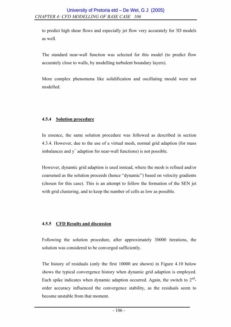
4.5.5 CFD Results and discussion

Following the solution procedure, after approximately 30000 iterations, the

solution was considered to be converged sufficiently.

The history of residuals (only the first 10000 are shown) in Figure 4.10 below

shows the typical convergence history when dynamic grid adaption is employed.

Each spike indicates when dynamic adaption occurred. Again, the switch to 2nd-

order accuracy influenced the convergence stability, as the residuals seem to

become unstable from that moment.

- 106 -



To ensure that the solution has truly converged, the maximum turbulent kinetic

energy (TKE)13 on the meniscus is displayed in Figure 4.11 as a function of each

iteration. The convergence of a physical property of the CFD model towards a

steady value, coinciding with sufficient and significant residual drops, constitutes

a converged solution. The failure of the maximum meniscus TKE to reach a

steady value (Figure 4.11) provides an indication of the possible unsteady nature

of the solution. A time accurate transient simulation is required to verify this,

although the water modelling experiments tend to indicate that the flow field is

steady.

Admittedly, the residuals for the 3D CFD model of the base case (presented in

Figure 4.10) suggest that the solution might not be converged. However, the

following reasons might be blamed:

• The flow seems to be pseudo-transient, as also reflected by Figure 4.11.

Pseudo-transient flow has been experienced to be more pronounced with

wider mould widths, as the history of residuals is much more stable and

convergent with narrower width moulds (3D exploration study in Chapter

5).

• The dynamic mesh adaption methods used (in an effort to control mesh

sizes) seem to prohibit the residuals from stabilising. As soon as the

solution starts to converge, the grid changes and the residuals are

simultaneously enlarged. More work on dynamic adaption methods is

necessary in future work.

The mesh quality is outstanding (100% hexahedral cells), and is thus not

suspected as being the main culprit, although this possibility cannot be ruled out

completely.

13 In Chapter 5, this measurement will play a significant role in the objective function during the optimisation of the SEN.

- 107 -



Figure 4.10: Residuals history (as a function of iteration number)

2nd-order

Figure 4.11: Physical property (maximum TKE on meniscus) as a function of iteration number

is noticeable in Figure 4.11 that there is noise in the physical measured property

(maximum TKE on meniscus in this case) as the solution progresses. If a certain

Iteration

Max

TK

E (m

2 /s2 )

It

- 108 -



property were to be used as part of the objective function for optimisation

purposes (Chapter 5), the specific property would need to be averaged in order to

obtain a more representative value.

The results of the 3D CFD half model are displayed symmetrically in Figures 4.12

4.20, in the form of:

ures 4.12 and 4.13)

• symmetry plane (Figure

• rs of temperature on the symmetry plane (Figure 4.17)

magnitude

and

The r ed in

Figure 21.

eatures of the jet and its three-dimensional shear layers can be

iscerned when comparing these results. E.g., path lines (Figure 4.18) and velocity

to

• contours of velocity and vorticity magnitude on the symmetry plane (i.e.,

centre plane) (Fig

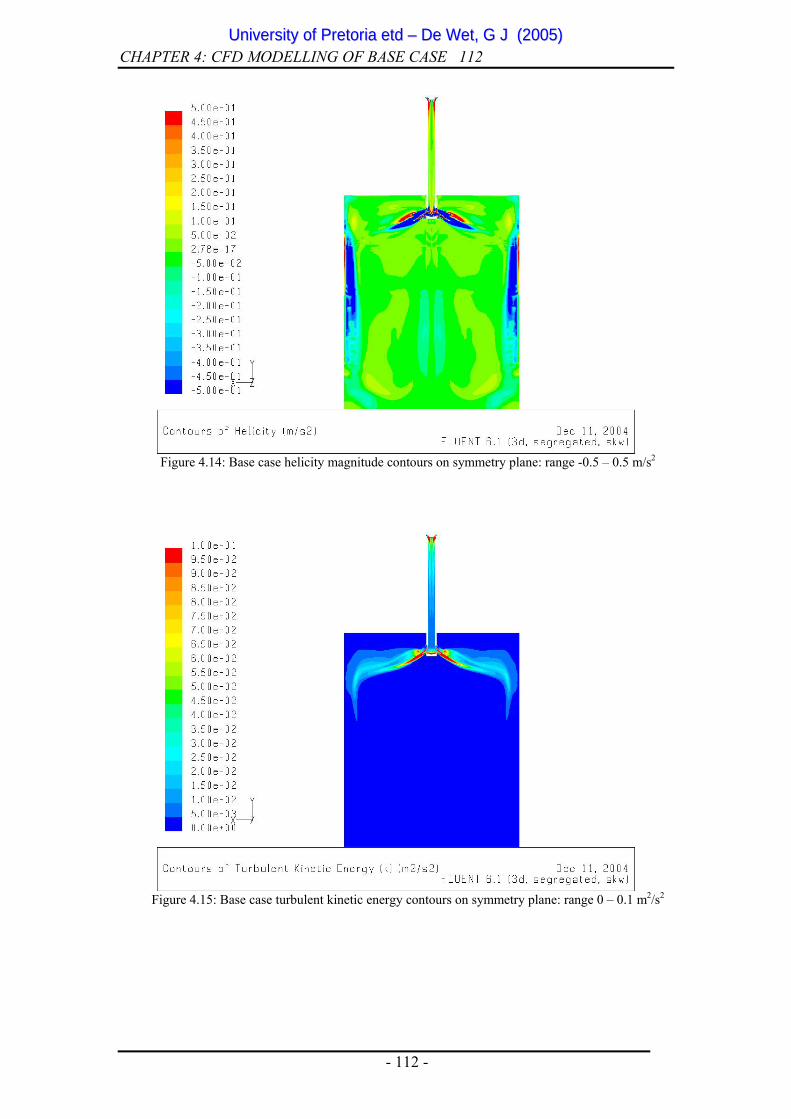
• contours of helicity14 on the symmetry plane (Figure 4.14)

contours of turbulent kinetic energy (TKE) on

4.15)

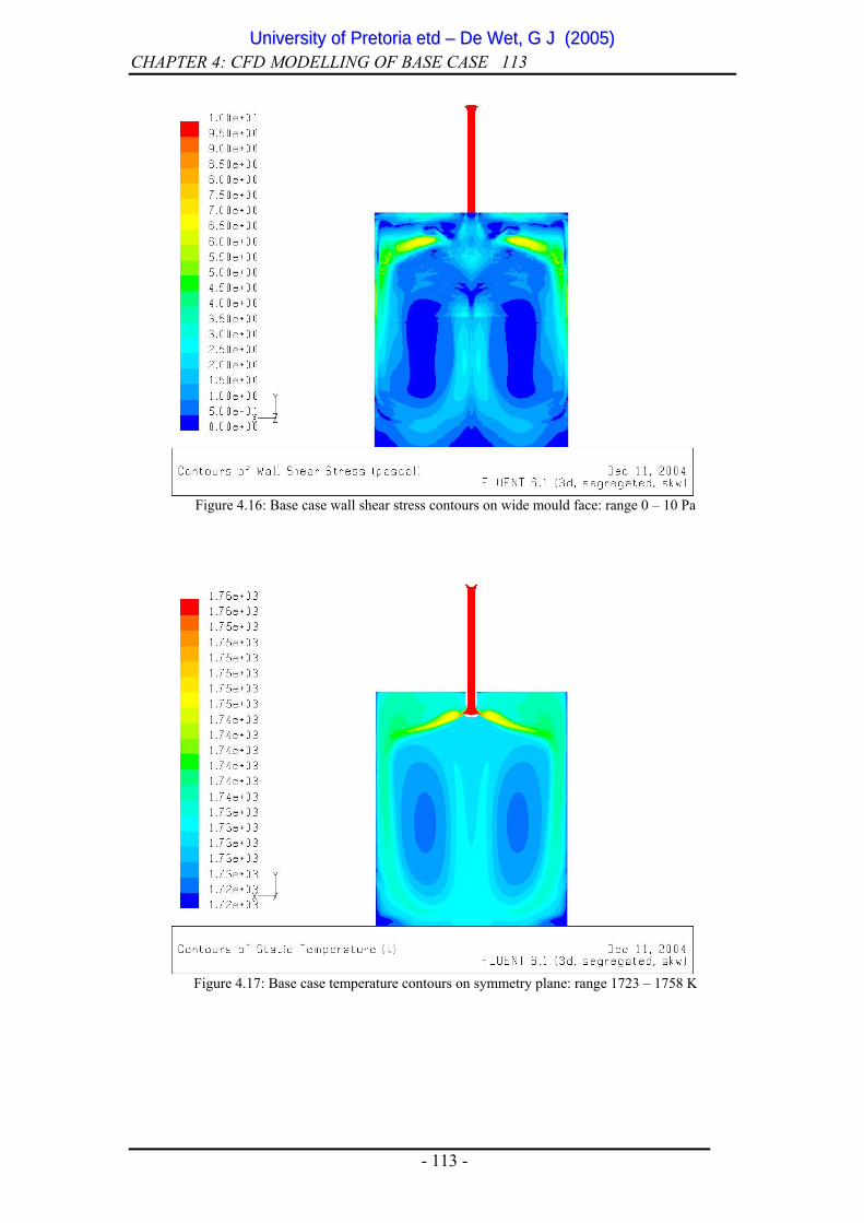
• contours of shear stress on the wide mould walls (Figure 4.16)

contou

• path lines originating from the SEN inlet, coloured by vorticity

(Figure 4.18)

• iso-surfaces of velocity magnitude coloured by turbulent kinetic energy

(Figure 4.19),

• velocity vectors scaled and coloured by its magnitude (Figure 4.20).

tu bulent kinetic energy on the meniscus surface (plan view) is display

Different f

d

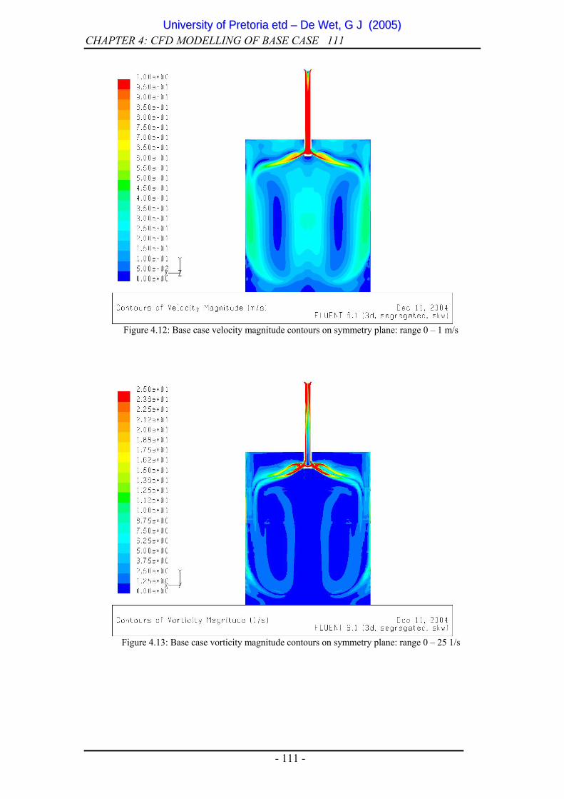
vectors (Figure 4.20) illustrate recirculating behaviour, whereas vorticity

magnitude (Figure 4.13) shows the extent of the jet shear layer. The impingement

location (important to prevent breakouts if this location is below the mould exit) is

most clearly depicted using path lines and helicity contours (Figure 4.14).

14 Helicity identifies the core of streamwise longitudinal vortices. By definition, normalised helicity represents the cosine of the angle between velocity and the vorticity vectors. The sign of helicity is dependent on the orientation of the local velocity vector relative to the vorticity vector. Thus the core of a streamwise vortex can be identified as the region of high helicity. Boundary layers are regions of high vorticity and low helicity [10].

- 109 -



The turbulent kinetic energy contours (Figure 4.15) show that the kinetic energy is

mostly concentrated inside the jet, as expected.

Figure 4.12, displaying contours of velocity magnitude on the centre plane of the

3D model, does not illustrate the true 3D nature of the flow, and the flow appears

be purely 2-dimensional.

place inside the mould: the yellow areas on the mould

all indicate that the jet dissipates (and lifts) as it propagates along the wall

rculating zones above jet exits). The iso-

rface of velocity magnitude contour (Figure 4.19) confirms the strange jet

n on the mould walls is satisfied, where

e mould walls are at the lowest temperature (in the accompanying temperature

to

However, the wall shear stress contours (Figure 4.16) clearly indicate the 3D

nature of the flow that takes

w

towards the narrow mould wall. This corresponds to the initial water model

experiments discussed in section 4.4.1.

The path lines (Figure 4.18) further illustrate the 3D flow patterns, as well as the

complexity of the flow (secondary reci

su

behaviour highlighted by the path lines and shear stress walls figures: the “ends”

of the jet lift up as the jet moves through the mould towards the narrow wall. It is

evident from this figure that the jet centre line (on the centre plane of the mould)

is lower than the sides or ends of the jet.

Figure 4.17, displaying contours of temperature magnitude on the centre plane,

clearly shows that the boundary conditio

th

scale), corresponding to the steel liquidus temperature (1723 K or 1450 ºC). As

expected, the (high) temperature of the jet is rapidly dissipated into the mould

cavity. The double recirculation zones (upper and lower) are also easily spotted in

this figure.

- 110 -



Figure 4.12: Base case velocity magnitude contours on symmetry plane: range 0 – 1 m/s

Figure 4.13: Base case vorticity magnitude contours on symmetry plane: range 0 – 25 1/s

- 111 -



Figure 4.14: Base case helicity magnitude contours on symmetry plane: range -0.5 – 0.5 m/s2

Figure 4.15: Base case turbulent kinetic energy contours on symmetry plane: range 0 – 0.1 m2/s2

- 112 -



Figure 4.16: Base case wall shear stress contours on wide mould face: range 0 – 10 Pa

Figure 4.17: Base case temperature contours on symmetry plane: range 1723 – 1758 K

- 113 -



Figure 4.18: Base case path lines coloured by vorticity magnitude: range 0 – 25 1/s (isometric

view)

Figure 4.19: Base case iso-surface of velocity magnitude (v=0.25m/s) coloured by turbulent kinetic

energy: range 0 – 0.1 m2/s2

- 114 -



Figure 4.20: Base case velocity vectors coloured by velocity magnitude: range 0 – 1 m/s (isometric

view)

The turbulent kinetic energy on the meniscus surface is shown in Figure 4.21,

illustrating the approximate positions where the maximum TKE occurs on the

meniscus. The figure is of a specific iteration and changes with each iteration

(refer to Figure 4.11), and appears to be transient in nature. In Chapter 5, the

maximum TKE on the meniscus surface will play a significant role in the

optimisation process of the SEN and mould.

- 115 -



Figure 4.21: Base case turbulent kinetic energy contours on meniscus surface: range 0 – 0.001

m2/s2 (top view)

4.6 CFD SEN and mould model: reduced widths

The initial base case and starting point of this study involved the 1575mm width

slabs, as Columbus Stainless (a major initiator of the study topic) experienced the

most quality problems on this width (their maximum width). As mentioned earlier in

this chapter, a number of problems regarding the CFD modelling resulted in so-called

unphysical flow solutions. Some inconsistencies still exist with models of the widest

width.

However, recently Columbus Stainless requested an optimum SEN design specifically

for narrower slab widths (range 1000mm – 1300mm)15. Naturally, CFD models of

these narrower widths were carried out, with surprising results:

15 Owing to availability of ADVENT full-scale water model results (also verified with UP 40%-scaled water model results), the widths 1060mm and 1250mm were chosen as representative for the 1000 – 1300mm range.

- 116 -


CHAPTER 4: CFD MODELLING OF BASE CASE 117 The 1060mm and 1250mm width results corresponded closely to water model

validation (full-scale and 40%-scaled) results.

Refer to Figure 4.22 showing the good correspondence between the 3D CFD model

velocity magnitude contours with the 40% water model test.

1060mm width; 80mm submergence depth; 1.1m/min casting d

UP 40% water model CFD k-ω turb model Figure 4.22: Comparison: Old SEN 40%-scaled water model with 3D CFD model (contours of

velocity) on centre plane

An interesting observation was that the submergence depth does not have a major

influence on the jet angle – it is mostly determined by the SEN design (port height,

angle, amongst others). Figure 4.23 clearly illustrates this point: the CFD model at a

(full-scale) submergence of 80mm, visualised using path lines, corresponds accurately

to the jet pattern of the 40%-scaled water model, at a much deeper submergence depth

of 150mm (full-scale). The SEN design used in Figure 4.23 is the base case (old SEN)

as described in section 4.2 of this chapter.

- 117 -



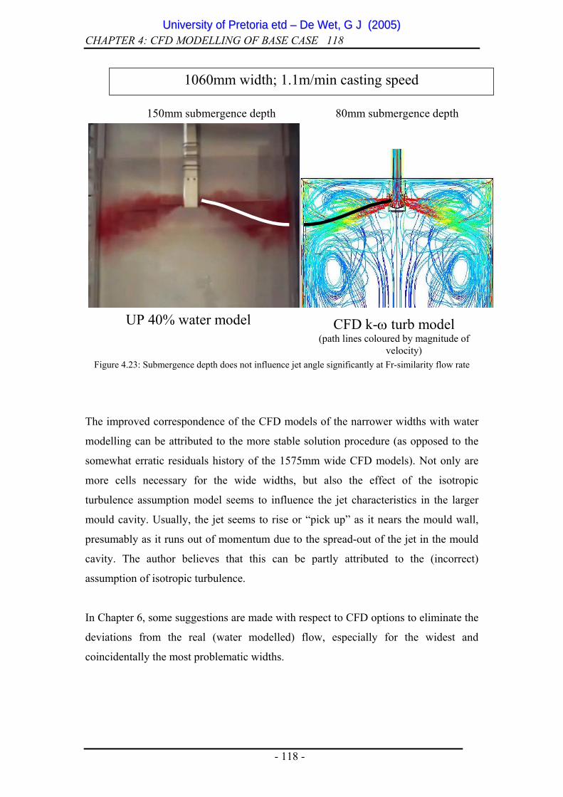
1060mm width; 1.1m/min casting speed

UP 40% water model CFD k-ω turb model (path lines coloured by magnitude of

velocity)

150mm submergence depth 80mm submergence depth

Figure 4.23: Submergence depth does not influence jet angle significantly at Fr-similarity flow rate

The improved correspondence of the CFD models of the narrower widths with water

modelling can be attributed to the more stable solution procedure (as opposed to the

somewhat erratic residuals history of the 1575mm wide CFD models). Not only are

more cells necessary for the wide widths, but also the effect of the isotropic

turbulence assumption model seems to influence the jet characteristics in the larger

mould cavity. Usually, the jet seems to rise or “pick up” as it nears the mould wall,

presumably as it runs out of momentum due to the spread-out of the jet in the mould

cavity. The author believes that this can be partly attributed to the (incorrect)

assumption of isotropic turbulence.

In Chapter 6, some suggestions are made with respect to CFD options to eliminate the

deviations from the real (water modelled) flow, especially for the widest and

coincidentally the most problematic widths.

- 118 -



- 119 -

4.7 Conclusion of base case CFD modelling

This chapter has illustrated CFD modelling of the SEN and mould base case as the

stepping-stone towards SEN optimisation with CFD.

A typical approach to any CFD simulation problem was illustrated using a diagram.

This approach was applied to the base case for this dissertation, which is the SEN

currently used by Columbus Stainless, Middelburg, South Africa:

Firstly, the base case was described in detail and certain assumptions were motivated

(e.g., simultaneous SEN and mould modelling, 2D vs. 3D modelling, etc.). Thereafter,

the CFD set-up was described, including choice of mesh elements, boundary

condition assumptions, choice of turbulence model, the solution procedure, to name

but a few. A momentum-only model was created to mimic water model conditions for

initial water model validation purposes.

After being confident that the CFD modelling of the water model was accurate, the

next step was to extend the CFD model to be able to imitate the real steel plant

circumstances. The solution of the full-scale CFD model of the real plant base case

was illustrated using a number of visualisation techniques. The (possible) transient

nature of the flow was also highlighted, which should be taken into account for

optimisation purposes (by averaging the properties that will be used for the objective

function/s). Furthermore, it was shown that reduced mould widths resulted in a more

stable flow field (of the CFD solution), which also confirms the fact that Columbus

Stainless experiences the most quality problems with their largest slabs with a width

of 1575mm.

In conclusion: the CFD modelling approach (including CFD set-up and solution

procedure) to typical SEN and mould applications was perfected and optimised for the

base case and other similar cases. These methods were verified by validating the CFD

solutions with water model experiments. Optimisation using these CFD modelling

techniques follows in the next chapter.


chapter 4: cfd modelling and base case verification

Documents