CHAPTER 4: ANGLES & DIRECTIONS

Definitions

Meridians longitude lines

True meridians converge to meet at the pole.

Grid meridians parallel to the central (true) meridian.

Magnetic meridian using magnetized needles that points to the magnetic North.

Horizontal angles deviation from the North direction or meridians.

Measured by Vernier transit (20")

Theodolite (1")

Vertical Angles are referenced to:

The horizon by plus (up) or minus (down) angles.

The zenith: directly above the observer.

The nadir: directly below the observer.

Q 1. Indicate which angles shown in the above figure are horizontal angles.

Vertical Angles are used in slope distance corrections

in height determination

Traverse: is a continues series of measured lines. Lines are measured by lengths and angles, and

defined by coordinates.

Closed polygons (traverse)

Sum of interior angles = (n - 2) 180

Sum of exterior angles = (n + 2) 180

281 10’ + 217 11’ + 220 59’ + 284 21’ + 256 19’

= 1258 120’ = 1260

Deflection angle:

From the prolongation of the back line to the forward line measured either to left (L) or to right

(R).

Azimuths & Bearings

Azimuth: Direction of a line given by the angle measured clockwise from the North meridian.

Range: 0 - 360

Q1. Calculate the Azimuths of lines 1-4.

Bearing: Acute angle between N-S meridian and the line measured clockwise or counterclockwise.

(1) N # # # E

(2) S # # # E

(3) S # # # W

(4) N # # # W

Q2. Calculate the Bearings of lines 5 - 8.

Relationship between Bearings and Azimuths

To convert from Azimuths to Bearings

NE quadrant: Bearing = Azimuth

SE quadrant: Bearing = 180 - Azimuth

SW quadrant: Bearing = Azimuth - 180

NW quadrant: Bearing = 360 - Azimuth

To convert from Bearings to Azimuths

NE quadrant: Azimuth = Bearing

SE quadrant: Azimuth = 180 - Bearing

SW quadrant: Azimuth = 180 + Bearing

NW quadrant: Azimuth = 360 - Bearing

Q3. Convert calculated Azimuths of lines 1 – 4 to Bearings, and convert calculated Bearings of lines 5 –

8 to Azimuths.

Reverse directions of lines

To reverse Bearing:

Reverse direction letters

AB BA

N S

S N

E W

W E

and angles stay as is.

To reverse Azimuth

if Azimuth < 180 add 180

if Azimuth 180 Subtract 180

Azimuth Computations

1: Check interior angles sum = (n - 2) 180

2: Counterclockwise (recommended)

a- reverse Azimuth

b- add next interior angle

c- go to start and check

3: Clockwise

a- find the Azimuth of the starting line (going clockwise)

b- reverse Azimuth

c- subtract interior angle

d- go to start to check

Note: you may need to add 360 to computations to facilitate subtraction.

Example: Find the azimuths of all the lines of the traverse.

1- Check sum of interior angles = (n - 2) 180

of internal angles = 7850’ + 14249’ + 1391’ + 7539’ + 10341’ = 54000’

(n - 2) * 180 = (5 – 2) *180 = 54000’ OK

2: Counterclockwise solution

Line AB

Az AB = 360 00’ - 7850’ = 28110’

Az BA = 28110’ - 18000’ = 10110’

+ B = 14249’

Az BC = 24359’

Az CB = 24359’ - 18000’ = 6359’

+ C = 13901’

Az CD = 20300’

Az DC = 20300’ - 18000’ = 2300’

+ D = 7539’

Az DE = 9839’

Az ED = 9839’ + 18000’ = 27839’

E = 10341’

Az EA = 38220’ = 2220’

Az AE = 2220’ + 18000’ = 20220’

A = 7850’

Az AB 28110’ OK.

Q1. Solve the same problem in a clockwise solution.

Bearing Computations

Computations solely depend on the trigonometric relationships.

The solution can proceed in either clockwise or anticlockwise procedures.

There is no systematic method for bearings computations.

Each bearing computation is regarded asd a separate problem.

A neat and a well labeled diagram should accompany each computation.

Example: Find the azimuths of all the lines of the traverse.

Soln.:

1- Line AB

N 58 W

2- Line BC

<X = 180 – 140 = 40

Bearing Angle = 180 – 58 - 40 = 82

BC = S 82 W

3- Line CD

<X = 180 – 128 = 52

Bearing Angle = 180 – 98 - 52 = 30

BC = S 30 W

4- Line DE

<X = 30 Why?

Bearing Angle = 180 – 84 - 30 = 66

BC = S 66 E

5- Line EA

<X = 66 Why?

<Y = 180 - 120 = 60

Bearing Angle = 180 – 60 - 66 = 54

BC = N 54 E

Q1. Solve the same problem in a clockwise solution, and compare your answers with the obtained ones.

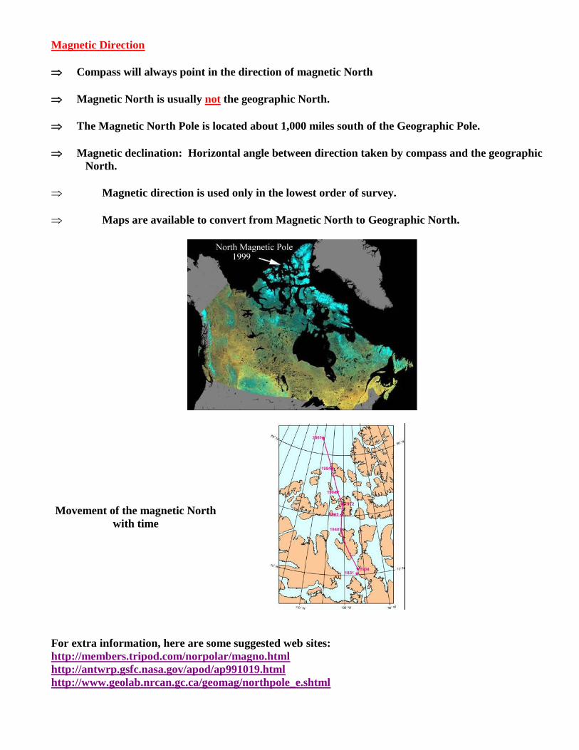
Magnetic Direction

Compass will always point in the direction of magnetic North

Magnetic North is usually not the geographic North.

The Magnetic North Pole is located about 1,000 miles south of the Geographic Pole.

Magnetic declination: Horizontal angle between direction taken by compass and the geographic

North.

Magnetic direction is used only in the lowest order of survey.

Maps are available to convert from Magnetic North to Geographic North.

Movement of the magnetic North

with time

For extra information, here are some suggested web sites:

http://members.tripod.com/norpolar/magno.html

http://antwrp.gsfc.nasa.gov/apod/ap991019.html

http://www.geolab.nrcan.gc.ca/geomag/northpole_e.shtml

Chapter 5: Theodolites/Transits

Older versions were called Transits. Nowadays, both words (Transits and Theodolites) are used

interchangeably.

Usage

Measure horizontal angles (deviation from the North).

Measure vertical angles (deviation from horizon, Nadir, or Zenith).

Establish straight lines.

Establish horizontal and vertical distances by using stadia.

Establish difference in elevation when used as leveling machine.

Major Parts

Alidade Assembly: includes telescope, vertical circle and vernier, horizontal verniers to read

horizontal angle, and clamps.

Circle Assembly: consists of a horizontal circle that has a hole to fit the spindle of the alidade

into it.

Leveling Head: were the circle assembly fits on.

Note: the circle assembly has two clamps

Upper clamp: to tighten the alidade to the circle

Lower clamp: to tighten the circle to the leveling head.

Targets: are plates having their center marked.

Types of Theodolites

In terms of measuring operation:

Repeating instruments:

Can be zeroed, measure 1, 2, 3, …

The circle assembly has two clamps (upper & lower)

Direction instruments:

Can not be zeroed.

The circle assembly has just one clamp (upper)

In terms of model:

Engineer transit:

Old

USA

Horizontal setting 0zenith

Optical theodolite (Repeating):

New

USA & other countries

Horizontal setting 90 or

270 zenith

0 zenith could be at the zenith

or Nadir

Electronic Theodolites:

Similar to optical theodolites

Precision is high

Digital readouts (no

interpolation)

Zero-set buttons

Horizontal angles can be turned

left or right

Automatic repeat - angle

averaging

Add EDM Total Station

How to check if the theodolite is measuring in Nadir, Zenith, or from Horizon?

Put telescope in a horizontal position and tilt it slightly up and check reading:

If reading close to zero Reading from horizon

If < 90 Zenith

If > 90 Nadir

Measuring Horizontal Angles

Turning the angle at least twice (plunging\transiting the telescope) will eliminate mistakes, most

instrument errors, and increase precision.

A. Directional Theodolites: Directional Theodolites can’t be zeroed.

1. Theodolite at A

2. While instrument at Face-Left (FL), vertical circle on the left side of surveyor, target telescope at "L"

point and record reading in the column FL (a) corresponding to point L.

ST PT Position I

(FL)

Position II

(FR) Mean Angle

A

L 276° 14’23”

(a)

96° 14’ 34”

(d) 276° 14’ 28”

31° 37’ 09”

R 307° 51’ 33”

(b)

127° 51’ 41”

(c) 307° 51’ 37”

3. Go clockwise and target at "R" point and record reading in the column FL (b) corresponding to point

R. The difference in the readings in the “FL” Column will be nearly equal to the value of the angle.

4. Plunge (transit) the telescope, now the instrument is Face Right (FR), vertical circle on the right side of

surveyor.

5. While still targeting on "R", record reading in the column FR corresponding to point R (c). The difference

between the FL and FR readings for the same point should be around 180.

6. Go anticlockwise and target on point "L" and record reading in the column FR corresponding to point L.

8. In the “Mean” column, take the mean of the minutes and seconds for each point and take the degrees for that

point either from the FL or FR column. You have to stick to one of the positions, FL or FR, in the whole table

for taking the degrees values.

9. The angle value is calculated by getting the difference between the two values in the “Mean” column.

10. The angle LÂR can be obtained by calculating difference in angels from position I (FL) and position II (FR).

ST. PT. POSITION I (F.L.) POSITION II (F.R.)

A

L 276° 14’ 22” 96° 14’ 34”

R 307° 51’ 33” 127° 51’ 41”

Difference 31° 37’ 11” 31° 37’ 07”

Mean 31° 37’ 09”

B. Repeating Theodolites

Repeating theodolites can be zeroed.

1. Theodolite at A

2. Zero instrument and target L

3. Go clockwise and target R

4. Record in (Direct)

5. Plunge telescope disengage lower motion gear

6. Target at L, record in (Direct)

7. Go clockwise and target R and record double

8. Take mean of double

ST Direct Double Mean =

Angle

A 13° 20’12” 26° 40’ 28” 13° 20’ 14”

Example 1:

ST Direct Double Mean =

Angle

A 78° 49’23” 157° 39’

08” 78° 49’ 34”

B 142° 49’53” 285° 38’ 28” 142° 49’ 14”

C 139° 00’17” 278° 01’ 56” 139° 00’ 48”

D 75° 39’12” 151° 17’ 56” 75° 38’ 58”

E 103° 41’10” 207° 22’ 28” 103° 41’ 14”

Summation 539° 59’ 58”

Correct Summation of angles = (n-2) * 180

= 3 * 180 = 540° 00’

Angular error of closure = 540° 00’ 00" - 539° 59’ 58”

= 02"

Measuring Vertical Angles

Vertical angles are angles measured in the vertical plane with zero or reference being a horizontal or

a vertical line. That is, a vertical angle is not measured from a low point to a high point, but from the

horizontal to the high point, a (+ve

) vertical angle or an angle of elevation, and from the horizontal to the low

point, a (-ve

) vertical angle or an angle of depression.

Vertical angles are referred to the vertical line in modern instruments and called zenithal angles (or

zenithal distances). If the angle lies between 0° and 90°, it is an angle of elevation (+ve

), otherwise it is an

angle of depression (-ve

) (between 90° and 180°).

Vertical angles are subject to index error which results from:

a. Displacement of the vertical circle

b. Lack of adjustment of the vertical circle reading device.

The index error is eliminated by sighting in two positions.

Measurement Procedure

1. Sight while the theodolite is in position I (Face Left) with the horizontal hair bisecting the target.

2. Center the bubble of the index level (match both ends in case of split bubble levels). This step is not

needed in theodolites with automatic vertical collimation.

3. Take the reading and record it (87° 22’ 43

”).

4. Reverse the telescope to position II (Face Right) and repeat steps 1, 2, and 3. Record the reading

(272° 39’ 57”).

5. Add both readings and compare the results with 360°. The difference (0° 2’ 40

”) is twice the value of

the index error.

6. Correct the readings such that their sum agrees with 360° exactly (87° 21’ 23” + 272° 38’ 37”= 360°

00’ 00”).

7. Subtract the corrected angle of position I from 90° to get the vertical angle (90° 00’ 0” - 87° 21’ 23”

= + 2° 38’ 37”).

PT. POSITION I POSITION

II SUM

INDEX

ERROR

VERTICAL

ANGLE

P5 87° 22

’ 43”

87° 21’ 23”

272° 39’ 57”

272° 38’ 37”

360° 02’ 04”

360° 00’ 00”

- 0° 1’ 20” +2° 38’ 37”

Field Application

I. Laying Out Angles

i) Laying out external angles:

Given Line AB required to layout line BC @ 3120'10"

Procedure:

1- Set Theodolite at B.

2- Sight on A and zero Theodolite.

3- Plunge (transit) telescope and turn required angle (3120'10").

4- Locate point C’.

5- Hold the angle reading and sight again on A.

6- Release the angle reading, plunge the telescope and turn it the required angle again. The reading

will be double the angle value (6240'20").

7- Locate point C”.

8- Locate point C which is midway between C’ and C”.

ii) Laying out internal angles:

Laying out internal angles is a special case of external angles.

Q1. Write the procedure for laying out internal angles; include a sketch in your procedure.

II. Prolonging straight lines

Given Line AB required to prolong the line

Procedure:

1- Set Theodolite at B and sight on A.

2- Plunge telescope and locate point C’.

3- Rotate telescope and sight again on A.

4- Plunge telescope and locate point C”.

5- Locate point C which is midway between C’ and C”.

III. Interlining (Balancing in)

Interlining is establishing a straight line between two not inter-visible points.

Procedure:

1- Select a point “C” between the two points that you can see both points from it.

2- Roughly align C’ between A & B.

3- Sight at A.

4- Plunge telescope and locate point B’.

5- Measure BB’ & calculate CC’.

6- Shift Theodolite to C”.

7- Repeat steps 3 – 6 until A, B & C are aligned.

IV. Intersection of two straight lines

This is a common situation when the surveyor is required to locate the intersection point when laying

out intersecting streets with the main street.

Procedure:

1- Set Theodolite @ main street center line (T1) and locate tow points (B & C) on it (about 1 m

apart) to be on both sides of the intersection point.

2- Stretch a string between points B & C.

3- Move the Theodolite to the center line of the crossing street (T2).

4- Align the telescope with the center line.

5- The instrument man is now in a position to find the intersection point between his view sight and

the stretched string.

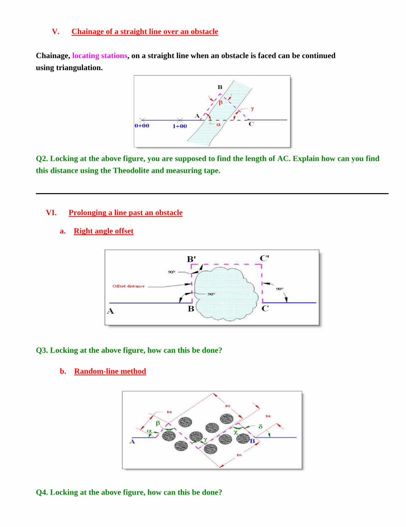
V. Chainage of a straight line over an obstacle

Chainage, locating stations, on a straight line when an obstacle is faced can be continued

using triangulation.

Q2. Locking at the above figure, you are supposed to find the length of AC. Explain how can you find

this distance using the Theodolite and measuring tape.

VI. Prolonging a line past an obstacle

a. Right angle offset

Q3. Locking at the above figure, how can this be done?

b. Random-line method

Q4. Locking at the above figure, how can this be done?

c. Triangulation Method

Using equilateral triangle.

Q5. Locking at the above figure, how can this be done?

Chapter 6: Traverse Surveys

Traverse: is a control survey which is a series of established stations that are tied together by angles

and distances.

Uses: (1) Locate topographic detail

(2) Layout engineering work

(3) Processing earth work.

Types: Close Traverse.

Open Travers.

Open Traverse

A series of measured straight lines and angles that do not geometrically close.

No geometric verification of stations

So for field verifications:

Distances measure twice

Angles doubled

When traverse stations can be tied to control monuments (BM’s) or by using accurate GPS then

verification is possible becomes Closed Travers.

Field notes of the above drawing

Station Direct Double Mean L/R

0+00 90° 00’ 180° 00’ 90° 00’ N 90° 00’ E

2+64 25° 12’ 50° 26’ 25° 13’ R

5+12 42° 20’ 84° 38’ 42° 19’ L

9+57 30° 56’ 61° 52’ 30° 56’ R

Chainages

Direct Reverse Mean Corrected

Chainage

0+00

264.3 264.5 264.4 2+64.4

248.1 248.0 248.1 5+12.5

445.4 445.8 445.6 9+58.1

235.7 235.9 235.8 11+93.9

Closed Traverse

Begins and ends at the same points

(Loop traverse)

Begins and ends at points of known position

Balancing Angles:

This is the first step in Traverse calculation

Interior angle sum = (n - 2) 180

Distribute error equally, arbitrary or according to weights (recommended).

Acceptable angular closure error is usually quite small (i.e., < 03')

Example:

Balance the following traverse.

Point Angle Value Correction Corrected Angle

A 78 49' (7849' / 540) * 03' =

+ 00 00' 26" 78 49' 26"

B 142 49' (14249' / 540) * 03' =

+ 00 00' 48" 142 49' 48"

C 139 01' + 00 00' 46" 139 01' 46"

D 75 37' + 00 00' 25" 75 37' 25"

E 103 41' + 00 00' 35" 103 41' 35"

Total 539 57' + 00 03' 540 00' 00"

Latitudes and Departures

Latitude: North/South rectangular component of a line

N = +ve

S = ve

Departure: East/West rectangular component

E = +ve

W = ve

Latitude (y) = dist (H) cos

Departure (x) = dist (H) sin

where, H horizontal dist of Traverse course

is Azimuth (sign is automatically corrected)

or

Bearing (sign must be entered).

Q1. In a tabular form calculate the latitudes and departures of the following lines.

In a perfect (or corrected) survey work;

+ve Latitudes = -ve Latitudes

+ve Departures = -ve Departures

Error of Closure & Precision

To find Linear Error of Closure (LEC) and Accuracy of a Traverse:

1. Balance the angles

2. Find azimuth (or bearing) of all traverse sides.

Points Angle Azimuth Bearing

A 78 50’

281 10’ N 78 50’ W

B 142 49’

243 59’ S 63 59’ W

C 139 01’

203 00’ S 23 00’ W

D 75 39’

98 39’ S 81 21’ E

E 103 41’

22 20’ N 22 20’ E

A 78 50’

3. Find latitudes (y) and departures (x)

Point Angle Length

(m) Azimuth Bearing

Latitude

(y) =

Hcos

Departure

(y) = H

sin

A 78 50’

11.39 281 10’ N 78 50’

W 2.21 -11.17

B 142 49’

9.86 243 59’ S 63 59’

W -4.32 -8.86

C 139 01’

8.29 203 00’ S 23 00’

W -7.63 -3.24

D 75 39’

18.35 98 39’ S 81 21’ E -2.76 18.14

E 103 41’

13.52 22 20’ N 22 20’ E 12.52 5.01

A 78 50’

540 00’ 61.41 0.02 -0.12

Note that in the above table, you have to end up with the same angle you have started with. We have started

and ended the table with point A.

Linear Error of Closure = LEC =

=

= 0.12

Accuracy Ratio = LEC / H = 0.12 / 61.41

= 1 / 511.75 = 1 / 500

The total error in the latitudes = 0.02

The total error in the departures = -0.12

Therefore, you have to subtract these errors from the latitudes and departures (according to

there weights) to have the corrected latitudes and departures.

Correction in Latitudes = Clat = - latitudes = - 0.02

Correction in departures = Cdep = - departures = 0.12

If we draw the measured traverse to scale on a paper by starting from point A going counter

clockwise to B, C, D, E then back to A, we find that starting A doesn't match ending A. This is

due to the error of closure.

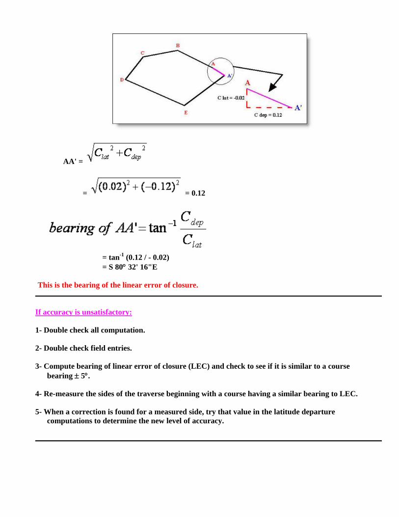
AA' =

= = 0.12

= tan-1

(0.12 / - 0.02)

= S 80 32' 16"E

This is the bearing of the linear error of closure.

If accuracy is unsatisfactory:

1- Double check all computation.

2- Double check field entries.

3- Compute bearing of linear error of closure (LEC) and check to see if it is similar to a course

bearing 5.

4- Re-measure the sides of the traverse beginning with a course having a similar bearing to LEC.

5- When a correction is found for a measured side, try that value in the latitude departure

computations to determine the new level of accuracy.

Accuracy ratio not enough for ensuring accuracy!

Errors might cancel each other

So in addition to accuracy ratio:

Check max allowable error in angle Ea

Check overall max allowable angular error

=Ea

Example 1.

For 5 sided traverse and linear accuracy 1/3000, find the allowable error in angles and overall max

allowable angular error.

Ea = = tan1

(1/3000)

Ea = 0.0191 = 1.1' = 1'

Overall allowable error = Ea = 1' = 2'

Error in any angle Ea 1'

and

Total error in all angles 2'

Transverse Adjustment:

Compass rule adjustment for lat & dep:-

Correction in Lat = (error in Lat)

Correction in Dep = (error in Dep)

where,

H side length (Horizontal distance)

P perimeter length ()

Latitudes and departures correction of the previous example

Point Angle Length

(m) Azimuth Bearing

Latitude

(y) =

Hcos

Departure

(x) =

H sin

Clat Cdep Balanced

Latitude

Balanced

Departure

A 7850’

11.39 281 10’ N 7850’ W 2.21 -11.17 - 0.02*

(11.39/61.41)

= - 0.004

+ 0.12*

(11.39/61.41)

= + 0.022

2.21 -11.15

B 14249’

9.86 243 59’ S 6359’ W -4.32 -8.86

- 0.02*

(9.86/61.41) = - 0.003

+ 0.12*

(9.86/61.41) = + 0.019

-4.32 -8.84

C 13901’

8.29 203 00’ S 2300’ W -7.63 -3.24 = - 0.003 = + 0.016 -7.63 -3.22

D 7539’

18.35 98 39’ S 8121’ E -2.76 18.14 = - 0.006 = + 0.036 -2.77 18.18

E 10341’

13.52 22 20’ N 2220’ E 12.52 5.01 = - 0.004 = + 0.026 12.52 5.04

A 7850’

54000’ 61.41 - 0.02 + 0.12 0.00 0.00

Correction of Original Traverse Data

AB (corrected) =

= = 11.37

= N 78 54' W

Point Angle Length

(m) Azimuth Bearing

Latitude

(y) =

Hcos

Departure

(x) =

H sin

Balanced

Latitude

Balanced

Departure

Corrected

Distance Corrected Bearing

A 7850’

11.39 281 10’ N 7850’ W 2.21 -11.17 2.21 -11.15 11.37 N 78 54’ W

B 14249’

9.86 243 59’ S 6359’ W -4.32 -8.86 -4.32 -8.84 9.84 S 63 57’ W

C 13901’

8.29 203 00’ S 2300’ W -7.63 -3.24 -7.63 -3.22 8.28 S 22 53’ W

D 7539’

18.35 98 39’ S 8121’ E -2.76 18.14 -2.77 18.18 18.39 S 81 20’ E

E 10341’

13.52 22 20’ N 2220’ E 12.52 5.01 12.52 5.04 13.50 N 22 56’ E

A 7850’

54000’ 61.41 - 0.02 + 0.12 0.00 0.00

Adjusted Coordinates Computed from Raw-Data Coordinates (introduction):

(1) Use original Azimuth, Distance, y, and x to find Northing and Easting coordinates.

(2) Adjust the computed Northing and Easting coordinates.

Good procedure for large computations using computers.

Coordinates Computation

Rectangular coordinates define the position of a point with respect to two perpendicular axes.

Coordinates using analytical geometry can be used for further computations.

In surveys where a coordinate grid system is not available, assume the X & Y axes in a position

to have positive coordinates of all stations.

Start the coordinates computation by assuming a large value for the starting station, (i.e.,

1000.00, 1000.00).

In your tabulation, start and end with the starting station.

Check that you have got the calculated coordinates of the starting station equal to the assumed

ones.

Latitudes and departures correction of the previous example

Point Angle Length

(m) Azimuth Bearing Lat. Dep.

Corrected

Latitude

Corrected

Departure Northing (y) Easting (x)

A 78 50’ 1000.00 1000.00

11.39 281 10’ N 7850’ W 2.21 -11.17 2.21 -11.15

B 14249’ 1000.00+2.21 =

1002.21

1000-11.15 =

988.85

9.86 243 59’ S 63 59’ W -4.32 -8.86 -4.32 -8.84

C 13901’ 1002.21-4.32 =

997.89

988.85–8.84 =

980.01

8.29 203 00’ S 23 00’ W -7.63 -3.24 -7.63 -3.22

D 75 39’ 990.26 976.79

18.35 98 39’ S 81 21’ E -2.76 18.14 -2.77 18.18

E 10341’ 987.49 994.97

13.52 22 20’ N 2220’ E 12.52 5.01 12.52 5.04

A 78 50’ 1000.00 1000.00

54000’ 61.41 - 0.02 + 0.12 0.00 0.00

Coordinate calculation is OK; since the assumed coordinate of point A is equal to its calculated

coordinate.

Missing Measurements

Due to presence of obstacles like trees, water tunnel, or highway, sometimes it is difficult to directly

measure one side of the traverse.

The technique of latitudes and departures can be used to find that side, and complete the traverse.

The idea is to arrange the sides in a form of closed traverse with one side missing.

Mainly you have to stick to a certain direction (clockwise or counterclockwise) in naming and

solving the traverse.

Example 1. Find the missing course in the following traverse:

Point Length

(m) Bearing Azimuth

Latitude

(y) =

Hcos

Departure

(x) = H

sin

A

261.27 N 31 22’ E

How? 31 22’ + 223.09 + 135.99

B

322.78 N 79 11’ E 79 11’ + 60.58 + 317.05

C

517.66 S 19 59’ W 199 59’ - 486.49 - 176.91

D

-202.82 + 276.13

Corrected + 202.82 - 276.13

A ?? ?? + 202.82 - 276.13

61.41 0.02 -0.12

Note that we have stuck with the direction and that distances are placed in the cells between the points.

DA =

Note it is DA not AD. Why?

= = 342.61

= N 53 42' W

Geometry of Rectangular Coordinates

Equation of line P1P2:

(1)

Length of line P1P2 = (2)

(3)

Slope of line P1P2 = = Cot

= 1/tan m (4)

From (1) & (4)

= Cot (5)

y - y1 = Cot (x - x1) (6)

Line to line of (6):

y - y1 = - tan (x - x1) (7)

Equations (6) & (7) are same equation except the slope term (m) is ( -1 / m)

dep. = H sin

lat. = H cos (9)

Equation of Circular Curve:

(x - H)2 + (y - K)

2 = r

2 (10)

Where: r radius, and H, K coordinate of the center

Equation of Circular Curve If center at origin

x2 + y

2 = r

2 (11)

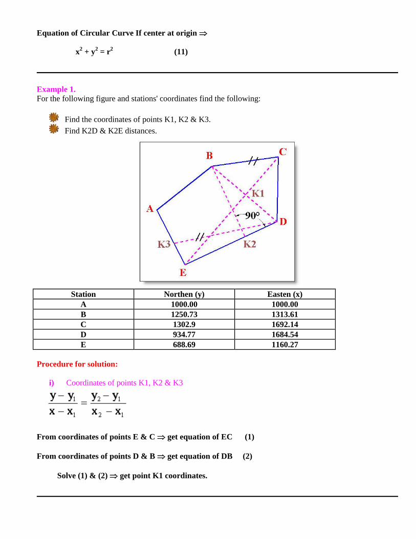
Example 1. For the following figure and stations' coordinates find the following:

Find the coordinates of points K1, K2 & K3.

Find K2D & K2E distances.

Station Northen (y) Easten (x)

A 1000.00 1000.00

B 1250.73 1313.61

C 1302.9 1692.14

D 934.77 1684.54

E 688.69 1160.27

Procedure for solution:

i) Coordinates of points K1, K2 & K3

From coordinates of points E & C get equation of EC (1)

From coordinates of points D & B get equation of DB (2)

Solve (1) & (2) get point K1 coordinates.

From coordinates of points E & D get equation of ED (3)

y - y1 = m (x – x1)

Equation of BK2 y - y1 = -1/m (x – x1) (4)

Solve (3) & (4) get point K2 coordinates.

From coordinates of points C & B get equation of CB

y – 1302.96 = (-52.23 / -378.53) (x – 1692.14)

(-52.23 / -378.53) = slope of BC = m = slope of DK3

Equation of DK3 y – Dy = m (x – Dx) (5)

From coordinates of points E & A get equation of EA (6)

Solve (5) & (6) get point K3 coordinates.

ii) K2D & K2E distances

Use coordinates of points K2, D & E

and l =

get K2D & K2E distances.

Q1. Numerically solve this example.

Example 2. From the information shown in the following figure, calculate the coordinates of the point of intersection (L)

of the centerlines of the straight and circular road sections.

Procedure for solution:

Since the coordinate values are very large which will cause significant rounding errors, it is

recommended to refer them to a transferred local coordinate system. At the end of solution, the

calculated coordinates will be referred back to the original coordinate system.

The transferred coordinate system will be at (316500.00, 4850.00).

Therefore the reduced coordinates are:

M (409.433, 277.101)

C (612.656, 317.313)

From the slope of the straight section and point M coordinates

Get the equation of the straight section. (1)

From the radius of the circular section and center coordinates

Get the equation of the circular section. (2)

Solve (1) & (2) get point L coordinates.

Q2. Numerically solve this example.

Area of Closed Traverse

Coordinate Method

Double Meridian Distance (DMD) Method

1- Area of Closed Traverse by Coordinate Method

Dividing the traverse area into two areas will give:

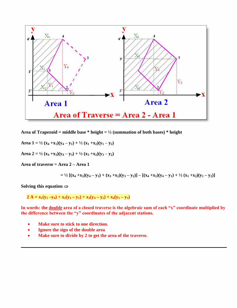
Area of Trapezoid = middle base * height = ½ (summation of both bases) * height

Area 1 = ½ (x4 +x1)(y4 – y1) + ½ (x1 +x2)(y1 – y2)

Area 2 = ½ (x4 +x3)(y4 – y3) + ½ (x3 +x2)(y3 – y2)

Area of traverse = Area 2 – Area 1

= ½ [(x4 +x3)(y4 – y3) + (x3 +x2)(y3 – y2)] – [(x4 +x1)(y4 – y1) + ½ (x1 +x2)(y1 – y2)]

Solving this equation

2 A = x1(y2 –y4) + x2(y3 – y1) + x3(y4 – y2) + x4(y1 – y3)

In words: the double area of a closed traverse is the algebraic sum of each “x” coordinate multiplied by

the difference between the “y” coordinates of the adjacent stations.

Make sure to stick to one direction.

Ignore the sign of the double area

Make sure to divide by 2 to get the area of the traverse.

Chapter 7: Topographic Surveys

Topographic surveys: used to determine the position and elevation of natural & manmade

features. These features can then be drawn to scale on a plan or map.

All topographic surveys are tied into both horizontal (X & Y reference grid) and vertical controls

(Bench Mark).

Scale and precision

1 : 100 1cm on map = 1 m on land

or

1" on map = 100" on land

Large scale Intermediate Small scale

1 : 100

1 : 200 1 : 2,000 1 : 20,000

1 : 500 1 : 5,000 1 : 50,000

1 : 1000 1 : 10,000 1 : 100,000

1 : 200,000

1 : 500,000

1 : 1,000,000

1 cm = 10 Km

Field precision should be compatible with possible on map plotting precision at the designated

map scale.

Example 1.

If points can be plotted to the closest 0.5 mm at scale 1:500

Then: Required field precision = 0.5 500 mm

= 250 mm = 0.25 m

Location by right-angle offsets:

Measuring:

i- distance from base line to the object (offset distance)

ii- measuring along the baseline to the point of perpendicularity.

Right angle using pentaprism

(double right angle prism)

The Double Right-Angle Prism 90

If a perpendicular line that is generally needed, the double right-angle prism is often the tool of choice. It is used when measuring cross-sections or setting slope stakes. This double right-angle prism consists of two pentagonal prisms

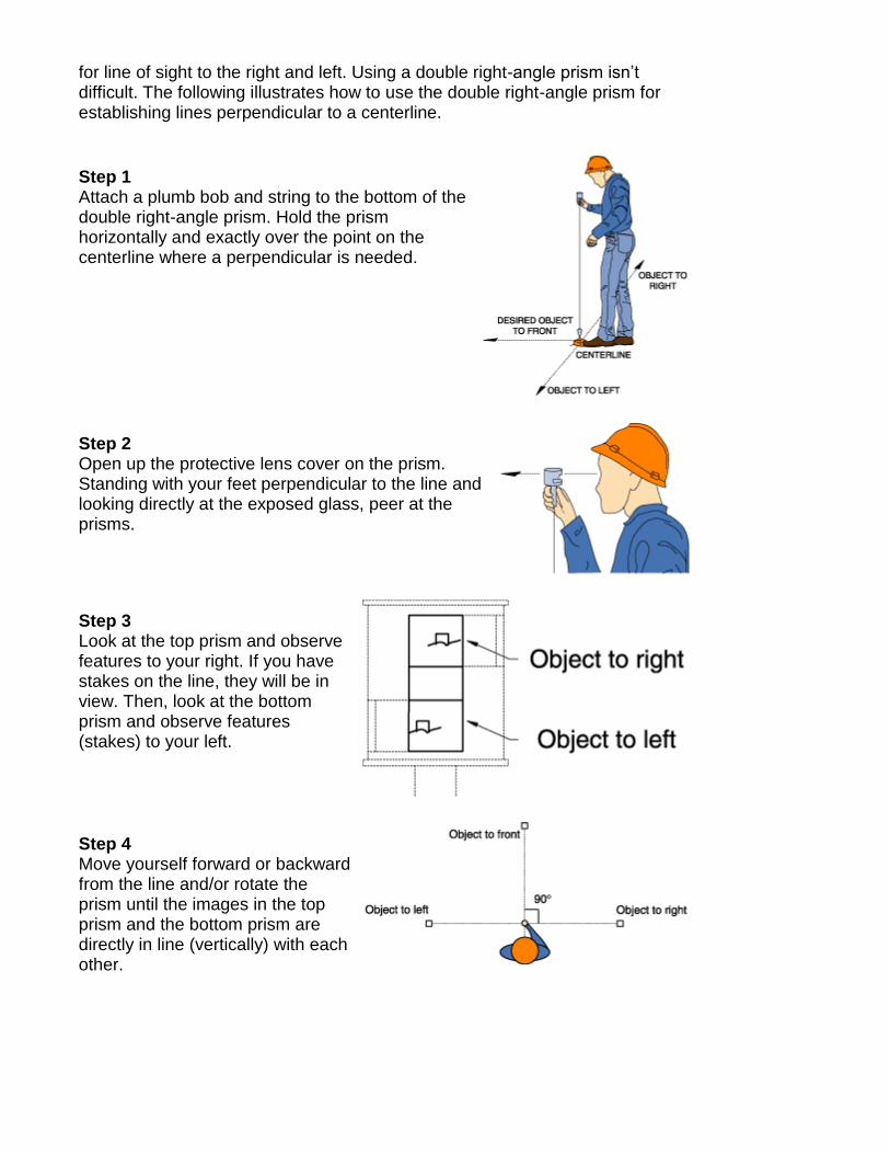
for line of sight to the right and left. Using a double right-angle prism isn’t difficult. The following illustrates how to use the double right-angle prism for establishing lines perpendicular to a centerline.

Step 1 Attach a plumb bob and string to the bottom of the double right-angle prism. Hold the prism horizontally and exactly over the point on the centerline where a perpendicular is needed.

Step 2 Open up the protective lens cover on the prism. Standing with your feet perpendicular to the line and looking directly at the exposed glass, peer at the prisms.

Step 3 Look at the top prism and observe features to your right. If you have stakes on the line, they will be in view. Then, look at the bottom prism and observe features (stakes) to your left.

Step 4 Move yourself forward or backward from the line and/or rotate the prism until the images in the top prism and the bottom prism are directly in line (vertically) with each other.

Step 5 When the top and bottom images are in a vertical line, communicate to your rod holder to move left or right until the rod being held is directly in line with the other images. When all three images are in a vertical line, the rod being held is perpendicular to the line. Tell your rod holder to mark the point. Thus, you have completed the double right-angle 90.

By Wesley G. Crawford, RPLS, is professor of building construction management at PurdueUniversity

Topographic survey can generate single or split baseline topographic details.

Double baseline topographic detail is used when the drawing becomes too congested. In this case the

horizontal control is split into two lines, just in the drawing, to show details in both

sides of the control line. The actual distance between the split lines is zero.

Cross Sections and Profiles

Profiles: a series of elevations taken along a baseline at some specified repetitive station interval.

Cross section: a series of elevations taken at right angles to a baseline at specific stations.

Stadia Principles

Tachometry technique (uses trigonometry calculation) to measure distances

Used in topographic surveys where accuracy is around 1/400

Uses the horizontal marks on the theodolite or level cross-hair

Stadia hairs are positioned in the reticle so that, if a rod is held 100m away from instrument, the

difference between upper and lower stadia hairs readings on a level rod is 1m

Horizontal distance (D) = Rod interval (S) * 100

If level or theodolite with leveled telescope in addition to the rod are used

Horizontal distance (D) = Rod interval(S) * 100

Elevation of B = Elevation of A + hi – RR

Q1. In the following figure, how can you tie point C to line AB (x, y, z) with one set of observations?

Inclined Stadia Measurements

If the stadia principle is applied when the rod is on a hilly area

The telescope will be inclined leading to error in the read interval

The rod interval of a sloped sighting must be reduced to what the interval would have been

if the line of sight had been perpendicular to the rod.

Fro the figure, the read interval is S’, while the corrected interval is S

S = S’ cos

D = 100 S

S = S’ cos

D = 100 S’ cos

H = D cos

H = 100 S’ cos2

V = D sin

D = 100 S’ cos

V = 100 S’ cos sin

Elevation of B = Elevation of A + hi + V – RR

The vertical distance (V) should be taken with its sign.

i.e., if A is lower than B the angle is an angle of inclination (+ve) leading to (+ve) V.

i.e., if A is higher than B the angle is an angle of depression (-ve) leading to (-ve) V.

Q 1. Calculate elevation of point A in the following figure:

Q 2. Calculate elevation of point A in the following figure:

Q 3. Calculate elevation of point A in the following figure:

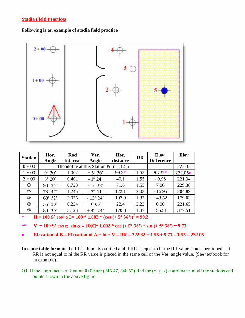
Stadia Field Practices

Following is an example of stadia field practice

Station Hor.

Angle

Rod

Interval

Ver.

Angle

Hor.

distance RR

Elev.

Difference

Elev

0 + 00 Theodolite at this Station & hi = 1.55 222.32

1 + 00 0 30’ 1.002 + 5 36’ 99.2* 1.55 9.73** 232.05

2 + 00 5 20’ 0.401 - 1 24’ 40.1 1.55 - 0.98 221.34

93 25’ 0.723 + 5 38’ 71.6 1.55 7.06 229.38

73 47’ 1.245 - 7 54’ 122.1 2.03 - 16.95 204.89

68 32’ 2.075 - 12 24’ 197.9 1.32 - 43.52 179.03

35 20’ 0.224 0 00’ 22.4 2.22 0.00 221.65

80 30’ 3.123 + 4224’ 170.3 1.87 155.51 377.51

* H = 100 S’ cos2 = 100 * 1.002 * (cos (+ 5 36’))

2 = 99.2

** V = 100 S’ cos sin * 1.002 * cos (+ 5 36’) * sin (+ 5 36’) = 9.73

Elevation of B = Elevation of A + hi + V – RR = 222.32 + 1.55 + 9.73 – 1.55 = 232.05

In some table formats the RR column is omitted and if RR is equal to hi the RR value is not mentioned. If

RR is not equal to hi the RR value is placed in the same cell of the Ver. angle value. (See textbook for

an example).

Q1. If the coordinates of Station 0+00 are (245.47, 348.57) find the (x, y, z) coordinates of all the stations and

points shown in the above figure.