chapter 4: a california nitrogen mass balance for...
TRANSCRIPT

California Nitrogen Assessment – Stakeholder review 27 June 2015
Chapter 4: A California nitrogen mass balance for 2005 1
Chapter 4: A California nitrogen mass balance for 2005 1
Lead authors: Dan Liptzin, Randy Dahlgren 2
Contributing author: Thomas Harter 3
4
Contents: 5
What is this chapter about? 6
Stakeholder questions 7
Main messages 8
4.0 Using a mass balance approach to quantify nitrogen flows in California 9
4.1 Statewide and subsystem nitrogen mass balances 10
4.1.1 Statewide nitrogen flows 11
4.1.2 Cropland nitrogen flows 12
4.1.2.1 Cropland N imports and inputs 13
4.1.2.2 Cropland N outputs and storage 14
4.1.3 Livestock nitrogen flows 15
4.1.3.1 Livestock feed 16
4.1.3.2 Livestock manure 17
4.1.4 Urban land nitrogen flows 18
4.1.4.1 Urban land imports and inputs 19
4.1.4.2 Urban land N outputs and storage 20
4.1.5 Household nitrogen flows 21
4.1.5.1 Human food 22

California Nitrogen Assessment – Stakeholder review 27 June 2015
Chapter 4: A California nitrogen mass balance for 2005 2
4.1.5.2 Human waste 23
4.1.5.3 Household pets 24
4.1.6 Natural land nitrogen flows 25
4.1.6.1 Natural land N imports and inputs 26
4.1.6.2 Natural land N outputs and storage 27
4.1.7 Atmosphere nitrogen flows 28
4.1.7.1 Atmosphere N imports and inputs 29
4.1.7.2 Atmosphere N exports and outputs 30
4.1.8 Surface water nitrogen flows 31
4.1.8.1 Surface water N inputs 32
4.1.8.2 Surface water exports, outputs and storage 33
4.1.9 Groundwater nitrogen flows 34
4.1.9.1 Groundwater inputs 35
4.1.9.2 Groundwater outputs and storage 36
4.2 Mass balance calculations and data sources 37
4.2.1 Fossil fuel combustion 38
4.2.2 Atmospheric deposition 39
4.2.3 Biological nitrogen fixation 40
4.2.3.1 Natural land N fixation 41
4.2.3.2 Cropland N fixation 42
4.2.4 Synthetic nitrogen fixation 43
4.2.4.1 Non-fertilizer synthetic chemicals 44
4.2.4.2 Synthetic fertilizer 45
4.2.5 Agricultural production and consumption: food, feed, and fiber 46

California Nitrogen Assessment – Stakeholder review 27 June 2015
Chapter 4: A California nitrogen mass balance for 2005 3
4.2.6 Manure production and disposal 47
4.2.7 Household waste production and disposal 48
4.2.8 Gaseous emissions 49
4.2.9 Surface water loadings and withdrawals 50
4.2.10 Groundwater loading and withdrawals 51
4.2.11 Storage 52
53
Boxes: 54
Box 4.1 Language used to categorize different N flows 55
Box 4.2 Language for describing absolute and relative N flows 56
Box 4.3 The problem of fertilizer accounting 57
Box 4.4 The Haber-Bosch process and cropland nitrogen 58
Box 4.5 Denitrification in groundwater 59
60
Figures: 61
Figure 4.1 Significant nitrogen flows in California, 2005 62
Figure 4.2 Land cover map of California, 2005 63
Figure 4.3 Measuring uncertainty in the California nitrogen mass balance 64
Figure 4.4a Statewide nitrogen imports to California in 2005 (1617 Gg N yr-1) 65
Figure 4.4b Statewide nitrogen exports and storage in California in 2005 (1617 Gg N yr-1) 66
Figure 4.5a Summary of nitrogen imports and inputs for the three California land subsystems in 67
2005 68
Figure 4.5b Summary of nitrogen outputs and storage for the three California land subsystems in 69
2005 70
California Nitrogen Assessment – Stakeholder review 27 June 2015
Chapter 4: A California nitrogen mass balance for 2005 4
Figure 4.6 Flows of nitrogen in California cropland in 2005 71
Figure 4.7 Flows of nitrogen in California urban land in 2005 72
Figure 4.8 Flows of nitrogen in California natural land in 2005 73
Figure 4.9 Relationship between wastewater treatment plant design flow and nitrogen discharge in 74
California 75
Figure 4.10 N imports and exports/storage per capita (Kg N person-1 yr-1) 76
Figure 4.11 N imports and exports/storage per unit area (Kg N ha-1 yr-1) 77
Figure 4.12 Relative contribution of N imports and exports/storage 78
79
Tables: 80
Table 4.1a California statewide nitrogen mass balance for 2005: imports 81
Table 4.1b California statewide nitrogen mass balance for 2005: exports and storage 82
Table 4.2 California cropland nitrogen mass balance in 2005 83
Table 4.3 Biological nitrogen fixation for agricultural crops in California in 2005 84
Table 4.4 Harvested nitrogen by crop 85
Table 4.5 Sources of data for biome-specific NO and N2O fluxes 86
Table 4.6 California livestock nitrogen mass balance in 2005 87
Table 4.7 Confined livestock populations and manure and animal food products for California in 88
2005 89
Table 4.8 Fate of manure nitrogen from confined livestock in California in 2005 90
Table 4.9 California urban land nitrogen mass balance in 2005 91
Table 4.10 Sources of nitrogen to landfills in California in 2005 92
Table 4.11 Fate of nitrogen in human excretion in California in 2005 93
Table 4.12 California natural land nitrogen mass balance in 2005 94
California Nitrogen Assessment – Stakeholder review 27 June 2015
Chapter 4: A California nitrogen mass balance for 2005 5
Table 4.13 Atmospheric nitrogen balance for California in 2005 95
Table 4.14 California surface water nitrogen mass balance in 2005 96
Table 4.15 Estimated annual N discharge to the ocean by watershed for California 97
Table 4.16 California groundwater nitrogen flows in 2005 98
Table 4.17 Major non-fertilizer uses of synthetic nitrogen in the United States 99
Table 4.18 Synthetic nitrogen consumption (Gg N yr-1) in the United States 100
Table 4.19 Assumed nitrogen content of animal products 101
Table 4.20 References for other nitrogen mass balance studies 102
103
104
105
106
107
108
109
110
111
112
113
114
115
116
California Nitrogen Assessment – Stakeholder review 27 June 2015
Chapter 4: A California nitrogen mass balance for 2005 6
What is this chapter about? 117
A mass balance of nitrogen inputs and outputs for California was calculated for the year 2005. This 118
scientifically rigorous accounting method tracks the size of nitrogen flows which allows us to understand 119
which sectors are the major users of nitrogen and which contribute most to the nitrogen in the air, 120
water, and ecosystems of California. New reactive nitrogen enters California largely in the form of 121
fertilizer, imported animal feed, and fossil fuel combustion. While some of that nitrogen contributes to 122
productive agriculture, excess nitrogen from those sources contributes to groundwater contamination 123
and air pollutants in the form of ammonia, nitric oxides, and nitrous oxide. In addition to statewide 124
calculations, the magnitude of nitrogen flows was also examined for eight subsystems: cropland; 125
livestock; urban land; people and pets; natural land; atmosphere; surface water; and 126
groundwater. Understanding the major nitrogen contributors will help policy makers and nitrogen users, 127
like farmers, prioritize efforts to improve nitrogen use. 128
129
Stakeholder questions 130
The California Nitrogen Assessment engaged with industry groups, policy makers, non-profit 131
organizations, farmers, farm advisors, scientists, and government agencies. This outreach generated 132
more than 100 nitrogen-related questions which were then synthesized into five overarching research 133
areas to guide the assessment (Figure 1.4). Stakeholder generated questions addressed in this chapter 134
include: 135
• What are the relative contributions of different sectors to N cycling in California? 136
• What are the relative amounts of different forms of reactive nitrogen in air and water? 137
• Are measurements of gaseous losses and water contamination accurate? 138
139
California Nitrogen Assessment – Stakeholder review 27 June 2015
Chapter 4: A California nitrogen mass balance for 2005 7
Main Messages 140
Synthetic fertilizer is the largest statewide import (519 Gg N yr-1) of nitrogen (N) in California. The 141
predominant fate of this fertilizer is cropland including cultivated agriculture (422 Gg N yr-1) and 142
environmental horticulture (44 Gg N yr-1). However, moderate amounts of synthetic fertilizer are also 143
used on urban land for turfgrass (53 Gg N yr-1). 144
145
The excretion of manure is the second largest N flow (416 Gg N yr-1) in California. The predominant 146
(72%) source of this N is dairy production, with minor contributions from beef, poultry and horses. A 147
large fraction (35%,) of this manure is volatilized as ammonia (NH3) from livestock facilities (97 Gg N yr-148
1) and after cropland application (45 Gg N yr-1). However, there is limited evidence for rates of ammonia 149
volatilization from manure. While liquid dairy manure must be applied very locally (within a few 150
kilometers (km) of the source), the solid manure from dairies and other concentrated animal feeding 151
operations can be composted to varying degrees and transported much longer distances (>100 km). 152
However, because of the increased regulation of dairies in the Central Valley (see Chapter 8), it will soon 153
be possible to determine what fraction of the dairy manure is used on the dairy farm compared to what 154
is exported based on the nutrient management plans produced for each dairy. 155
156
Synthetically fixed N dominates the N flows to cropland. Synthetic fertilizer (466 Gg N yr-1) is the 157
largest flow of N to cropland, but a large fraction of N applied in manure and irrigation water to 158
cropland is also originally fixed synthetically. On average, we estimated that 69% of the N added 159
annually to cropland statewide is derived from synthetic fixation. 160
161
The biological N fixation that occurs on natural land (139 Gg N yr-1) has become completely 162
overshadowed by the reactive N related to human activity in California. While this flow was once the 163

California Nitrogen Assessment – Stakeholder review 27 June 2015
Chapter 4: A California nitrogen mass balance for 2005 8
major source of new reactive (i.e., biologically available) N to California, it now accounts for less than 164
10% of new imports at the statewide level. The areal rate (8 kg N ha-1 yr-1) representing the sum of all N 165
inputs to natural lands, including N deposition, is an order of magnitude lower than either urban or 166
cropland. 167
168
The synthetic fixation of chemicals for uses other than fertilizer is a moderate (71 Gg N yr-1) N flow. 169
These chemicals include everyday household products such as nylon, polyurethane, and acrylonitrile 170
butadiene styrene plastic (ABS). These compounds have been tracked to some degree at the national 171
level (e.g., Domene and Ayres 2001), but the data were largely compiled in expensive and proprietary 172
reports. The true breadth and depth of their production, use, and disposal is poorly established. 173
174
Urban land is accumulating N. Lawn fertilizer, organic waste disposed in landfills, pet waste, fiber (i.e 175
wood products), and non-fertilizer synthetic chemicals are all accumulating in the soils (75 Gg N yr-1), 176
landfills (68 Gg N yr-1), and other built areas associated with urban land (122 Gg N yr-1). 177
178
Nitrogen exports to the ocean (39 Gg N yr-1) from California rivers accounts for less than 3% of 179
statewide N imports. In part, this low rate of export is due to the fact that a major (45%) fraction of the 180
land in California occurs in closed basins with no surface water drainage to the ocean. While 181
concentrations of nitrate in some rivers can be quite high, the total volume of water reaching the ocean 182
is quite low. 183
184
Direct sewage export of N to the ocean (82 Gg N yr-1) is more than double the N in the discharge of all 185
rivers in the state combined. Because of the predominantly coastal population, the majority of 186

California Nitrogen Assessment – Stakeholder review 27 June 2015
Chapter 4: A California nitrogen mass balance for 2005 9
wastewater is piped several miles out to the ocean. A growing number of facilities (> 100) in California 187
appear to be using some form of N removal treatment prior to discharge. 188
189
Nitrous oxide (N2O) production is a moderate (38 Gg N yr-1) export pathway for N. Human activities 190
produce 70% of the emissions of this greenhouse gas while the remainder is released from natural land. 191
Agriculture (cropland soils and manure management) was a large fraction (32%) of N2O emissions in the 192
state. 193
194
Ammonia is not tracked as closely as other gaseous N emissions because it is not currently regulated 195
in the state. While acute exposures to NH3 are rare, both human health and ecosystem health are 196
potentially threatened by the increasing regional emissions and deposition of NH3. However, rigorous 197
methods for inventorying emissions related to human activities as well as natural soil emissions are 198
currently lacking. 199
200
Atmospheric N deposition rates in parts of California are among the highest in the country, with the N 201
deposited predominantly as dry deposition. The Community Multiscale Air Quality model predicts that 202
66% of the deposition is oxidized N and 82% of the total deposition is dry deposition not associated with 203
precipitation events. In urban areas and the adjacent natural ecosystems of southern California, 204
deposition rates can exceed 30 kg N ha-1 yr-1, but deposition is, on average, 5 kg N ha-1 yr-1 statewide. 205
206
The atmospheric N emitted as NOx or NH3 in California is largely exported via the atmosphere 207
downwind (i.e., east) from California. Approximately 65% of the NOx and 73% of the NH3 emitted in 208
California is not redeposited within state boundaries making California a major source of atmospheric N 209
pollution. Further, atmospheric exports of N are more than 20 times higher than riverine N exports. 210

California Nitrogen Assessment – Stakeholder review 27 June 2015
Chapter 4: A California nitrogen mass balance for 2005 10
Leaching from cropland (333 Gg N yr-1) was the predominant (88%) input of N to groundwater. It 211
appears that N is rapidly accumulating in groundwater with only half of the annual N inputs extracted in 212
irrigation and drinking water wells or removed by denitrification in the aquifer. On the whole, 213
groundwater is still relatively clean, with a median concentration ~ 2 mg N L-1 throughout the state. 214
However, there are many wells in California that already have nitrate concentrations above the 215
Maximum Contaminant Level. Because of the time lags associated with groundwater transport (decades 216
to millennia), the current N contamination in wells is from past activities and current N flows to 217
groundwater will have impacts far into the future. 218
219
The amount of evidence and level of agreement varies between N flows. The most important sources 220
of uncertainty in the mass balance calculations are for major flows with either limited evidence or low 221
agreement or both. Based on these criteria, biological N fixation on cropland and natural land, the fate 222
of manure, denitrification in groundwater, and the storage terms are the most important sources of 223
uncertainty. 224
225
In many ways, the N flows in California are similar to other parts of the world. In a comparison with 226
other comprehensive mass balances - Netherlands, United States, Korea, China, Europe, and Phoenix - 227
California stands out in its low surface water exports and high N storage, primarily in groundwater and 228
urban land. Further, when compared to these other regions of varying size, California has a relatively 229
low N use on both a per capita, but especially on a per hectare, basis. 230

California Nitrogen Assessment – Stakeholder review draft 27 June 2015
Chapter 4: A California nitrogen mass balance for 2005 11
4.0 Using a mass balance approach to quantify nitrogen flows in California 231
Human activities, including agriculture and urban development, have led to dramatic increases in 232
biologically available or reactive nitrogen (N). As such, the anthropogenic alteration of the N cycle is 233
emerging as one of the greatest challenges to the health and vitality of California’s people, ecosystems, 234
and agricultural economy. Input of N to terrestrial ecosystems has more than doubled in the past 235
century due to nitrogen fixation associated with food production and energy consumption (Galloway 236
1998). This mobilization of anthropogenic N has been connected with increased N loading to aquatic 237
ecosystems, emissions of nitrous oxide (a greenhouse gas), and associated ecosystem and human-health 238
effects (Galloway et al. 2003). In some cases, the N flow itself is inherently a component of an 239
ecosystem service (e.g., harvesting N in crops is an essential part of food provisioning), while in other 240
cases N flows are more indirectly linked to impairing ecosystem services (e.g., excess nitrogen (i.e., 241
eutrophication)) in surface water bodies leads to hypoxia and harmful algal blooms). This chapter will 242
focus on the current state of N flows and the following chapter will address how the current N flows and 243
trends in N flows are affecting ecosystem services and human well-being in California. 244
A mass balance is an efficient and scientifically rigorous method to track the flows of N in a 245
system. The underlying premise of a mass balance is that all of the reactive N entering (i.e., inputs) the 246
study area must be exactly balanced by N leaving (i.e., outputs) and N retained in the study area (i.e., 247
change in storage): 248
N Inputs = N Outputs + ∆Storage 249
A mass balance approach is not only very useful to compare the size of N flows but also to identify gaps 250
in understanding the size and directions of these flows. Some flows are difficult to quantify – they are 251
highly variable in time and/or space, or there are simply no methodologies to easily measure or predict 252
the flows. Nevertheless, knowledge of the relative magnitude of the flows is needed to make informed 253
management and policy decisions for targeting N reductions. 254
California Nitrogen Assessment – Stakeholder review draft 27 June 2015
Chapter 4: A California nitrogen mass balance for 2005 12
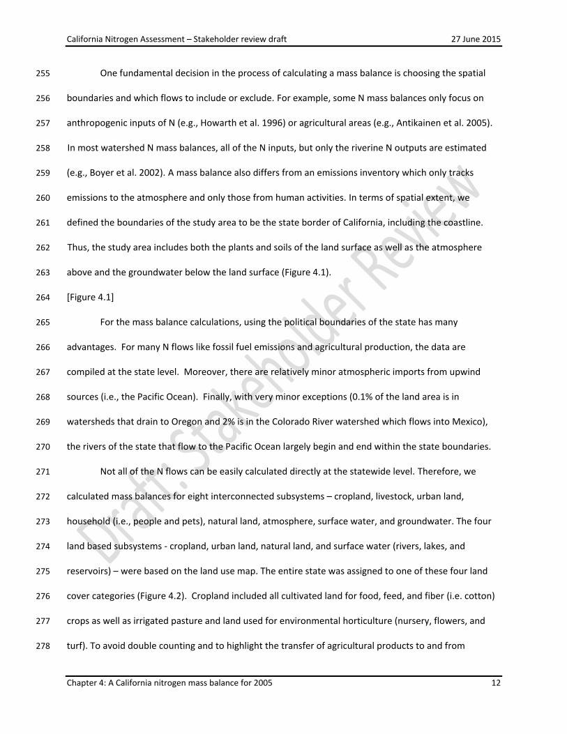
One fundamental decision in the process of calculating a mass balance is choosing the spatial 255
boundaries and which flows to include or exclude. For example, some N mass balances only focus on 256
anthropogenic inputs of N (e.g., Howarth et al. 1996) or agricultural areas (e.g., Antikainen et al. 2005). 257
In most watershed N mass balances, all of the N inputs, but only the riverine N outputs are estimated 258
(e.g., Boyer et al. 2002). A mass balance also differs from an emissions inventory which only tracks 259
emissions to the atmosphere and only those from human activities. In terms of spatial extent, we 260
defined the boundaries of the study area to be the state border of California, including the coastline. 261
Thus, the study area includes both the plants and soils of the land surface as well as the atmosphere 262
above and the groundwater below the land surface (Figure 4.1). 263
[Figure 4.1] 264
For the mass balance calculations, using the political boundaries of the state has many 265
advantages. For many N flows like fossil fuel emissions and agricultural production, the data are 266
compiled at the state level. Moreover, there are relatively minor atmospheric imports from upwind 267
sources (i.e., the Pacific Ocean). Finally, with very minor exceptions (0.1% of the land area is in 268
watersheds that drain to Oregon and 2% is in the Colorado River watershed which flows into Mexico), 269
the rivers of the state that flow to the Pacific Ocean largely begin and end within the state boundaries. 270
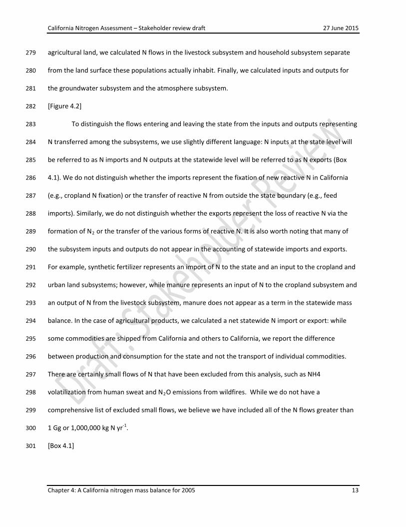
Not all of the N flows can be easily calculated directly at the statewide level. Therefore, we 271
calculated mass balances for eight interconnected subsystems – cropland, livestock, urban land, 272
household (i.e., people and pets), natural land, atmosphere, surface water, and groundwater. The four 273
land based subsystems - cropland, urban land, natural land, and surface water (rivers, lakes, and 274
reservoirs) – were based on the land use map. The entire state was assigned to one of these four land 275
cover categories (Figure 4.2). Cropland included all cultivated land for food, feed, and fiber (i.e. cotton) 276
crops as well as irrigated pasture and land used for environmental horticulture (nursery, flowers, and 277
turf). To avoid double counting and to highlight the transfer of agricultural products to and from 278
California Nitrogen Assessment – Stakeholder review draft 27 June 2015
Chapter 4: A California nitrogen mass balance for 2005 13
agricultural land, we calculated N flows in the livestock subsystem and household subsystem separate 279
from the land surface these populations actually inhabit. Finally, we calculated inputs and outputs for 280
the groundwater subsystem and the atmosphere subsystem. 281
[Figure 4.2] 282
To distinguish the flows entering and leaving the state from the inputs and outputs representing 283
N transferred among the subsystems, we use slightly different language: N inputs at the state level will 284
be referred to as N imports and N outputs at the statewide level will be referred to as N exports (Box 285
4.1). We do not distinguish whether the imports represent the fixation of new reactive N in California 286
(e.g., cropland N fixation) or the transfer of reactive N from outside the state boundary (e.g., feed 287
imports). Similarly, we do not distinguish whether the exports represent the loss of reactive N via the 288
formation of N2 or the transfer of the various forms of reactive N. It is also worth noting that many of 289
the subsystem inputs and outputs do not appear in the accounting of statewide imports and exports. 290
For example, synthetic fertilizer represents an import of N to the state and an input to the cropland and 291
urban land subsystems; however, while manure represents an input of N to the cropland subsystem and 292
an output of N from the livestock subsystem, manure does not appear as a term in the statewide mass 293
balance. In the case of agricultural products, we calculated a net statewide N import or export: while 294
some commodities are shipped from California and others to California, we report the difference 295
between production and consumption for the state and not the transport of individual commodities. 296
There are certainly small flows of N that have been excluded from this analysis, such as NH4 297
volatilization from human sweat and N2O emissions from wildfires. While we do not have a 298
comprehensive list of excluded small flows, we believe we have included all of the N flows greater than 299
1 Gg or 1,000,000 kg N yr-1. 300
[Box 4.1] 301

California Nitrogen Assessment – Stakeholder review draft 27 June 2015
Chapter 4: A California nitrogen mass balance for 2005 14
In addition to the spatial boundaries, it is important to consider temporal boundaries. Some 302
flows, like crop harvest, vary inter-annually with climate and other factors, but are measured every year. 303
Some N flows, like biological N fixation and gaseous soil emissions, tend to be average annual estimates 304
without reference to a particular time period. Finally, other flows, like atmospheric N deposition, are 305
estimated with data and computationally intensive methods and are only available for one year. Our 306
aim was to create a budget for 2005. For agricultural production, the averages were calculated for 2002-307
2007 while for most other N flows, any data available between the years 2000-2008 were used. The N 308
flows were calculated by compiling the necessary data from both peer-reviewed and non-peer reviewed 309
literature, government databases, and in some cases expert opinion. When possible, we calculated 310
multiple independent estimates of the N flows during this time period. A quantitative measure of 311
uncertainty is reported in Section 4.1 as part of the estimates of the N flows. 312
The concurrent goals of this mass balance were (1) to quantify current statewide N flows and (2) 313
to evaluate the scientific uncertainty in the magnitude of N flows. This chapter is divided into two 314
sections. The first section (Section 4.1) provides a summary of the statewide N imports and exports and 315
the N flows in the eight subsystems. Both the absolute and relative sizes of the N flows were grouped 316
into categories to help highlight which flows are particularly important (Box 4.2). The second section 317
(Section 4.2) provides a detailed description of the data sources and calculations used in the mass 318
balance. The spatial and temporal variability of important stocks and flows of N will be addressed in 319
detail in the Ecosystem Services and Human Well Being chapter (Chapter 5). 320
[Box 4.2] 321
Uncertainty in the mass balance is addressed in this chapter as well as the Data Tables. The 322
discussion in this chapter largely focuses on comparing multiple independent estimates of the same N 323
flow. In the data tables, we concentrate on the uncertaisnties associated with individual data sources 324
and methodologies. Following the model of the Intergovernmental Panel on Climate Change, we use 325

California Nitrogen Assessment – Stakeholder review draft 27 June 2015
Chapter 4: A California nitrogen mass balance for 2005 15
reserved words to quantify the level of scientific agreement and the amount of evidence (Box 1, Data 326
Tables). The uncertainties associated with each N flow depicted in Figure 4.1 are presented both in 327
Figure 4.3, in the various tables showing the state-level and subsystem mass balances, and in the Data 328
tables. 329
[Figure 4.3] 330
331
4.1 Statewide and subsystem N mass balances 332
This section describes the magnitude of the N flows at the statewide level as well as the eight 333
subsystems examined in the mass balance: cropland; livestock; urban land; household; natural land; 334
atmosphere; surface water; and groundwater. For the statewide flows of agricultural products, we 335
report net flows in the cases of food, feed, and fiber and not the transport of individual commodities. 336
We calculate the net flow as the difference between production and consumption. Based on our results, 337
feed and fiber represent statewide imports of N and food represents a statewide export of N. At the 338
statewide level, the California atmosphere was considered internal to the system with advection 339
resulting in N import to and export from the atmosphere. 340
341
4.1.1 Statewide N flows 342
There were six moderate to major statewide imports of N to California – synthetic N fixation, fossil fuel 343
combustion, biological N fixation, atmospheric imports (i.e. advection of N) feed, and fiber in the form of 344
wood products (Figure 4.1). Products created from synthetic N fixation by industrial processes, typically 345
by the Haber-Bosch process, represent the largest statewide import (590 Gg N yr-1) and a large (36%) 346
fraction of the new statewide imports (Table 4.1a, Figure 4.4a). Of this synthetically fixed N, the 347
predominant (88%) form was fertilizer. However, the mixture of other chemicals (e.g., nylon, 348
polyurethane, acrylonitrile butadiene styrene plastic) created from synthetically fixed NH3 also 349

California Nitrogen Assessment – Stakeholder review draft 27 June 2015
Chapter 4: A California nitrogen mass balance for 2005 16
represented a moderate (71 Gg N yr-1) N flow. Fossil fuel combustion was the second largest import (404 350
Gg N yr-1) of N to California with NOx the predominant (89%) form. This flow represents N emissions to 351
the atmosphere and is not equivalent to atmospheric N deposition in California (Section 4.1.7). 352
Biological N fixation was also a major statewide N import (335 Gg N yr-1) with more occurring on the 353
400,000 ha of alfalfa compared to the 33 million ha of natural land. While there was medium evidence 354
for this flow, there was low agreement. The import of livestock feed and fiber in the form of wood and 355
wood products to meet the demand in California represented major (200 Gg N yr-1) and moderate (40 356
Gg N yr-1) statewide imports of N, respectively. 357
[Table 4.1a; Figure 4.4a] 358
To satisfy the mass balance assumption, statewide N exports and storage were defined to be 359
equivalent to N imports at the statewide level. Atmospheric exports of N gases and particulate matter 360
were estimated based on the assumption of no N storage in the atmosphere. All nitrous oxide (N2O) and 361
nitrogen gas (N2) emitted was assumed to be exported from California while the export of NOx and NH3 362
was calculated as the difference of emissions and deposition to the land subsystems. The atmospheric N 363
export (NOx, NH3, N2O, and N2) accounted for the predominant (86%) fraction of the N exports from 364
California (Figure 4.4b, Table 4.1b). More NOx (270 Gg N yr-1) than NH3 (206 Gg N) was exported. Nitrous 365
oxide was a moderate (38 Gg N yr-1) statewide export of N while N2 represented a major statewide 366
export (204 Gg N yr-1). This total includes groundwater denitrification even though the N2 produced may 367
not reach the atmosphere for several decades until the groundwater is discharged at the surface. 368
Including groundwater denitrification, the inert N2 emissions account for 29% of the gaseous N export 369
from the state. While most of the NOx export was related to the N import related to fossil fuel 370
combustion, the export of the other gaseous forms represents N that was transformed within the state. 371
For example, a large fraction of the NH3 derives from manure, which previously was feed, which in turn 372
may have been imported to the state. California was a net exporter of food. That is, the total 373
California Nitrogen Assessment – Stakeholder review draft 27 June 2015
Chapter 4: A California nitrogen mass balance for 2005 17
production of N in food was 79 Gg N yr-1 greater than the estimated consumption of N in food. The 374
gross flow of food is likely significantly higher with many fresh fruits and vegetables as well as dairy 375
products transported out of the state. Moderate statewide exports of N to the ocean occurred in both 376
rivers (39 Gg N yr-1) and direct sewage discharge (82 Gg N yr-1). 377
[Table 4.1b; Figure 4.4b] 378
A large (43%) fraction of the N imports were stored in some form in California (701 Gg N yr-1). 379
Accumulation of N in groundwater was estimated to be 258 Gg N yr-1, with the input predominantly 380
from cropland. Storage in the soils or vegetation of the three land subsystems was estimated to be 230 381
Gg N yr-1. Within the urban subsystem, there was N storage associated with landfills (71 Gg N yr-1), but a 382
major (122 Gg N yr-1) source of storage was related to the buildup of synthetic chemicals and wood 383
products in structures and long-lived household items like nylon carpets, electronic equipment and 384
lumber. Finally, storage in surface water bodies (i.e. lakes and reservoirs) was 20 Gg N yr-1. We assumed 385
no storage in the atmosphere subsystem. 386
There are some examples of measured increases in N storage in California, but there is more 387
evidence related to carbon storage. Agricultural soils in California (Singer 2003) and turfgrass soils 388
(Raciti et al. 2011) have been shown to accumulate both carbon (C) and N. Ornamental lawns in 389
southern California were found to accumulate 1400 kg C ha-1 yr-1 for more than three decades after lawn 390
establishment (Townsend-Small and Czimzik 2010). Assuming a soil C:N ratio of 10, this would represent 391
140 kg N ha-1 yr-1, similar to the results of N accumulation reported by Raciti et al. (2011) for Maryland. 392
In other contexts, storage of N can be inferred from measurements of carbon storage. For example, the 393
increasing acreage of perennial crops in California (Kroodsma and Field 2006) results in net uptake of 394
carbon by ecosystems in California (Potter 2010). The disposal of organic materials like wood products 395
and food waste in landfills results in 10% of the total dry mass of solid waste sequestered in the form of 396
carbon (C) (Staley and Barlaz 2009). Depending on the chemical environment in the landfill and the C:N 397
California Nitrogen Assessment – Stakeholder review draft 27 June 2015
Chapter 4: A California nitrogen mass balance for 2005 18
ratio of the materials, varying amounts of N would be accumulating as well. With these multiple avenues 398
for C sequestration, it is very likely that N storage would be increasing as well in these settings. Some of 399
these storage pools (soils and vegetation) have an asymptotic capacity for N uptake which may be 400
saturated within years or decades. However, the disposal of waste in landfills and the use of long-lived 401
wood and synthetic materials can potentially keep increasing over time. The high capacity for retention 402
of N in surface water bodies is well established especially in reservoirs (e.g., Harrison et al. 2009), but 403
the fraction buried in sediments versus the fraction denitrified is not. 404
Nitrogen flows can also be tracked through the land-based subsystems: cropland, urban land, 405
and natural land. Because of the N flows among subsystems, the total sum of N inputs across all 406
subsystems was greater than the statewide N imports. For example, manure N was an input to the 407
cropland subsystem, but not an import to the state as it was considered a transformation of existing N 408
at the scale of California. Agriculture, including cropland and livestock, dominated the N inputs in 409
California (Figure 4.5a). Cropland had greater N inputs than urban land and natural land combined. 410
Similarly, livestock feed was more than double the amount of human and pet food. The two biggest 411
inputs to the three land subsystems were synthetic N fertilizer (to cropland and urban land) and manure 412
(to cropland). Less than half of the N inputs to cropland and one quarter of the N inputs to livestock 413
were converted into food or feed (Figure 4.5b). More than a third of cropland N inputs were leached to 414
groundwater and a similar fraction (40%) of livestock N inputs was emitted as ammonia. Other gaseous 415
N emissions from cropland and the other land subsystems were only minor N flows. Human food was 416
largely converted to sewage with the exception of the food waste that was disposed of in landfills. While 417
natural land and cropland were estimated to store small fractions of their N inputs, the predominant 418
fate of N inputs to urban land was storage in soils, landfills, or as long-lived synthetic materials or wood. 419
[Figure 4.5a; Figure 4.5b] 420
421

California Nitrogen Assessment – Stakeholder review draft 27 June 2015
Chapter 4: A California nitrogen mass balance for 2005 19
4.1.2 Cropland N flows 422
Cropland covers only 4.9 million of the 40.8 million hectares in California, but accounts a 423
disproportionate amount of the N flows (Table 4.2, Figure 4.6). A total of 1027 Gg N yr-1 was added to 424
cropland resulting in an average areal N input to cropland of 250 kg N ha-1 yr-1. 425
[Table 4.2; Figure 4.6] 426
427
4.1.2.1 Cropland N imports and inputs 428
The use of synthetic fertilizer on cropland represented the largest flow of N in California (Figure 4.6, 429
Table 4.2). The 2002-2007 average statewide synthetic N fertilizer sales were 762 Gg N yr-1. However, it 430
is unclear why there was nearly a 50% increase in sales from 2001-2002 or similarly a 50% increase from 431
the 1980-2001 mean to 2002-2007 mean fertilizer sales (Box 4.3). There was no significant linear change 432
(p=0.28) in fertilizer sales over the period 1980-2001. We believe that the mean from this period, 519 Gg 433
N yr-1, provides a more realistic estimate of statewide fertilizer sales than the 2002-2007 mean. The 434
fraction of fertilizer sales applied to cropland was calculated as the difference between turfgrass use (53 435
Gg N yr-1, see Section 4.1.4) and total fertilizer sales. Synthetic fertilizer use was therefore a major flow 436
of N (466 Gg N yr-1), representing a large (45%) fraction of total N flows to cropland soils. Manure 437
application was also a major (263 Gg N yr-1) N input to cropland (see Section 4.1.3). A large uncertainty 438
is related to the partitioning of manure between gaseous NH3 losses and application to cropland (Figure 439
4.3). In our accounting methodology we only considered synthetic N applied as fertilizer as a N import 440
(i.e., new input of N) in the budget calculations at the statewide scale. However, many of the other 441
sources of N to cropland (e.g., manure, irrigation, atmospheric deposition) also originally derive in part 442
from synthetic fertilizer applied to cropland (Box. 4.4). We assumed that half of the biosolids produced 443
in the state were applied to cropland soils. 444
[Box 4.3; Box 4.4] 445
California Nitrogen Assessment – Stakeholder review draft 27 June 2015
Chapter 4: A California nitrogen mass balance for 2005 20
Synthetic fertilizer applied to cropland can also be estimated based on the crop-specific 446
fertilization rates and harvested acreages. For the period 2002-2007, cultivated crops were estimated to 447
receive 539 Gg N yr-1. This value would be expected to be higher than the synthetic fertilizer sales data 448
for cropland if any manure was used as fertilizer. A total of 263 Gg N yr-1 of manure was estimated to be 449
applied to cropland. If 73 Gg N yr-1 of manure was used instead of synthetic fertilizer then the two 450
estimates would agree perfectly. While some manure likely does replace synthetic fertilizer to meet the 451
nutritional needs of crops, a significant fraction could have been applied in excess of plant needs on 452
dairy-forage crops as a form of waste disposal, or as an amendment to increase soil organic matter. 453
Synthetic fertilizer use in environmental horticulture was calculated separately because it relied 454
on different sources of data. There were 7,100 ha of sod, 6,200 ha of floriculture, and 13,100 ha of open 455
grown nursery stock which were estimated to receive 44 Gg N yr-1. 456
Biological N fixation was also a major (196 Gg N yr-1) flow to cropland and almost entirely 457
associated with alfalfa (Table 4.3). We were not aware of any N fixation rates for alfalfa measured in 458
California, where productivity, and thus N fixation, is much higher than the Midwestern states where 459
data have been collected. While there was variability associated with the productivity – N fixation 460
relationship, the biggest source of uncertainty in the estimate of N fixation is the amount of fixed N 461
belowground. 462
[Table 4.3] 463
Two moderate N flows to cropland are atmospheric deposition and N applied in irrigation water. 464
The total atmospheric deposition of N to cropland was estimated at 43 Gg N yr-1 based on the results of 465
the Community Multiscale Air Quality (CMAQ) model (Table 4.2). The mean N deposition rate for 466
cropland, 8.7 kg N ha-1 yr-1, was higher than the state average of 5.0 kg N ha-1 yr-1. Irrigation water 467
provided a similar quantity of N (59 Gg N yr-1) to cropland statewide as N deposition. Surface water was 468
withdrawn at a rate of 2.6*1013 L yr-1 for irrigation use in California in 2000 (Hutson et al. 2004). In 2000, 469
California Nitrogen Assessment – Stakeholder review draft 27 June 2015
Chapter 4: A California nitrogen mass balance for 2005 21
a total of 0.6 *1013 L yr-1 was pumped from the Sacramento-San Joaquin Delta (the Delta) at Tracy for 470
the Delta Mendota Canal and the California Aqueduct (Blue Ribbon Task Force Delta Vision 2008). 471
Because the Delta pumps are located downstream of the location of river gauges (which we consider to 472
be the boundary of the study area), this pumping resulted in the return of 8 Gg N yr-1 to the state. The 473
remaining surface water withdrawals for irrigation, calculated as the difference between total surface 474
water use and Delta pumping, provided another 18 Gg N yr-1 to cropland. Groundwater nitrate (NO3-) 475
concentrations (2.6 mg N L-1) were even higher than the N concentration in the water pumped from the 476
Delta. However, only 1.3 *1013 L yr-1 were pumped from groundwater in 2000 for irrigation, resulting in a 477
total of 33 Gg N yr-1. 478
479
4.1.2.2 Cropland N outputs and storage 480
Harvesting crops was a major flow of N and the largest N output from the cropland subsystem. The top 481
twenty crops in terms of harvested N are shown in Table 4.4. For 2002-2007, total harvest of food crops 482
was 185 Gg N yr-1 and feed crops was 357 Gg N yr-1. Cotton lint was the only fiber crop grown on 483
California cropland (timber was considered harvested from natural land), with only 1 Gg N yr-1 484
harvested. The production of nursery and floriculture crops was 14 Gg N yr-1. While there is transport of 485
this nursery material in and out of California, we estimate that CA produces 14% of the national total 486
and would use 12% based on its population resulting in no net flow of nursery material. 487
[Table 4.4] 488
The total production showed minimal variability over this time period with less than a 10% 489
difference between the lowest (2002) and highest (2003) quantity of N harvested. The two sources of 490
crop acreages, the county Agricultural Commissioners and National Agricultural Statistics Service (NASS) 491
annual surveys, were highly correlated (r > 0.95) for the common crops that are reported by both 492
agencies. The largest source of uncertainty in the crop calculations is in the conversion of production to 493
California Nitrogen Assessment – Stakeholder review draft 27 June 2015
Chapter 4: A California nitrogen mass balance for 2005 22
the N content of the biomass. The USDA crop nutrient tool is a compilation of data from several 494
decades ago, but no more recent database exists. The potential for large errors are greatest for the 495
forage crops where the whole plant is harvested and for the vegetables with high water content. 496
Gases were emitted from cropland soils as a result of both physical and biological processes. 497
Ammonia volatilization is a physical process based on the temperature and pH dependent equilibration 498
of gaseous NH3 and dissolved ammonium (NH4+) in the soil. Based on an emission factor of 3.2% for the 499
various synthetic fertilizers in California, as well as emissions from land applied manure, NH3 outputs 500
were a moderate flow (60 Gg N yr-1). The other gas outputs are associated with the microbial processes 501
of nitrification and denitrification. Based on the average of all sources of data (Table 4.5), nitric oxide 502
(NO) and N2O outputs were also minor flows (12 and 10 Gg N yr-1, respectively; Table 4.2). Using the 503
limited number of published literature estimates from California cropland soils, the median NO and N2O 504
fluxes were 1.9 kg NO-N ha-1 yr-1 and 2.9 kg N2O-N ha-1 yr-1, respectively (Supplementary 4.11). These 505
rates are considerably higher than the global median for NO (0.9 kg NO-N ha-1 yr-1) and N2O (1.4 kg N2O-506
N ha-1 yr-1) from the largest global compilation of gaseous emissions from cropland soils (Stehfest and 507
Bouwman 2006). The total emissions of N2O calculated from the California areal rates and cropland area 508
was 14 Gg N yr-1. This value is similar to the estimate of 9 Gg N yr-1 using the emissions factor approach. 509
Emissions of nitrogen (N2) gas from soils from denitrification were also a minor flow (17 Gg N yr-1), 510
estimated using a fixed N2:N2O ratio of 1.66. Because of the high variability in N2:N2O ratios and the 511
high reported rates measured in California in the 1970s, we estimated a lower and upper bound for the 512
N2:N2O as 1.25 and 2.31 as the mean ± 2 SE of the Schlesinger (2009) dataset. Taking into account the 513
uncertainty, the range of N2 emissions would be 13 to 23 Gg N yr-1. 514
[Table 4.5] 515
1 Supplementary materials will be available through the Agricultural Sustainability Institute’s website at www.nitrogen.ucdavis.edu.

California Nitrogen Assessment – Stakeholder review draft 27 June 2015
Chapter 4: A California nitrogen mass balance for 2005 23
Dissolved outputs of N to surface water from cropland were estimated based on a predicted N 516
yield (14 kg N ha-1 yr-1). As only 2.9 million ha of California cropland was located in watersheds with 517
surface water drainage, outputs of N to surface water (i.e., runoff) from cropland was a moderate N flow 518
(41 Gg N yr-1). Kratzer et al. (2011) reported similar N yields for the Central Valley sub-watersheds with 519
the highest fraction of agricultural land, the Orestimba Creek watershed (17.9 kg N ha-1) and the portion 520
of the San Joaquin River near Patterson (16.3 kg N ha-1). 521
Leaching below the rooting zone was a major flow (333 Gg N yr-1) of N from cropland. This value 522
is the average of two approaches which differ considerably in magnitude (Supplementary 4.2). 523
Multiplying recharge volume by the median concentration of NO3- from published studies in California 524
estimating leaching below the rooting zone, cropland leaching was estimated to be 395 Gg N yr-1. In 525
contrast, using the median of the fraction of applied fertilizer (synthetic + manure) that leaches from 526
published studies in California predicted only 272 Gg N yr-1 leached. Thus, the level of agreement on the 527
magnitude of N leaching is low. Conditions in the vadose zone in California are not conducive to 528
denitrification (Green et al. 2008a). Therefore, this leached nitrate would be predicted to reach the 529
groundwater table. Like many other fluxes, there was high spatial and temporal variability. However, 530
while it is relatively simple to measure NO3- concentrations in leachate, it is more difficult to estimate N 531
load as it also requires an estimate of the recharge volume. One recent estimate of leaching that 532
actually calculated the areal rate of N loading in recharge was nearly 100 kg N ha-1 yr-1 in an almond 533
orchard near the Merced River (Green et al. 2008b). Based on our statewide total N load and cropland 534
area, we estimated that the average areal rate of cropland N loading would be 68 kg N ha-1 yr-1. It is 535
possible to use models (e.g., Watershed Analysis Risk Management Framework, Soil and Water 536
Assessment Tool) to estimate nitrate leaching; however this approach is typically used for much smaller 537
regions than an entire state, or even the entire Central Valley, and requires a large number of 538
parameters to be estimated. 539

California Nitrogen Assessment – Stakeholder review draft 27 June 2015
Chapter 4: A California nitrogen mass balance for 2005 24
Based on the difference between inputs and outputs, soil storage was calculated as 65 Gg N yr-1. 540
There was limited evidence for storage of N in cropland soils in California. Based on the repeated 541
sampling of agricultural soils throughout California, on average, N content in cropland soils increased 542
from 0.9% to 0.29% in the upper 25 cm (Singer 2003). Assuming no change in bulk density over the 55 543
year period between samples, cropland soils would accumulate 1 kg N ha-1yr-1 for a total of 5 Gg N yr-544
1 statewide. This suggests that the estimate of storage by difference is too high. If we used the estimate 545
of soil storage and calculate leaching by difference, the N flow would be 395 N yr-1, equivalent to the 546
higher of the two estimates for leaching based on recharge volume and concentration. Based on data 547
from Post and Mann (1990), soils will accumulate carbon when carbon concentrations are less than 1% 548
in the top 15 cm, assuming an average soil bulk density of 1 g cm-3. Many of the agricultural areas in the 549
state, with the notable exception of the Delta, were established in areas with relatively low organic 550
matter soils. Therefore, increases in soil N would be expected as well. However, these increases in soil N 551
are not linear over time; with the highest increases expected soon after land conversion and saturating 552
after a certain time (e.g., Garten et al. 2011). 553
554
4.1.3 Livestock N flows 555
The N flows for the livestock subsystem assumed that all of the livestock in the state (with the exception 556
of beef cows and all calves) were on feed. 557
558
4.1.3.1 Livestock feed 559
The majority of crop production (357 Gg N yr-1) in California was harvested to feed livestock (Table 4.2). 560
However, this production must be supplemented with another 200 Gg N yr-1 of feed imported from out 561
of the state. Corn grain from the Midwest is a major source of livestock feed. The waybill samples from 562
the Surface Transportation Board suggest that over 300 million bushels of corn arrive in California 563
California Nitrogen Assessment – Stakeholder review draft 27 June 2015
Chapter 4: A California nitrogen mass balance for 2005 25
annually on trains originating in Nebraska and Iowa (US DOT 2010). This feed supply was converted into 564
141 Gg N yr-1 of food and 416 Gg N yr-1 of manure (Table 4.6). Dairy cows and replacement stock 565
dominated the demand for livestock feed and manure production, but beef cattle, poultry, and horses 566
contributed a significant fraction as well (Table 4.7). 567
[Table 4.6; Table 4.7] 568
569
4.1.3.2 Livestock manure 570
The majority of the N in livestock feed is excreted. Livestock manure is potentially a nutrient resource, 571
but concentrated quantities can pose a waste disposal problem (Table 4.8). The fraction of manure that 572
is volatilized as NH3 depends on the type of livestock. Using the US Environmental Protection Agency 573
(EPA) emission factors and our estimates of excretion, we calculated an emission of 97 Gg NH3-N yr-1. 574
from livestock facilities. When combined with manure-associated emissions from cropland (45 Gg NH3-575
N yr-1), this N flow is almost identical to the reported tonnage of NH3 in EPA (2004); however, this is far 576
larger than the value of 69 Gg N yr-1 in the 2005 EPA National Emissions Inventory for California (EPA 577
2008). While there is a high amount of evidence for the amount of manure excreted by livestock, there 578
is limited evidence for the fate of that manure. There are relatively few data measuring NH3 emissions 579
for the management practices and climate specific to California. Therefore, the emissions of NH3 and 580
the land application of manure are speculative (Figure 4.3). However, as the residence time of NH3 in 581
the atmosphere is relatively short, this reduced N may essentially be land applied from atmospheric 582
deposition downwind of dairy facilities. The underestimate of modeled compared to measured N 583
deposition in the ecosystems on the west slope of the Sierra Nevada could result from an underestimate 584
of NH3 emissions in the model. 585
[Table 4.8] 586

California Nitrogen Assessment – Stakeholder review draft 27 June 2015
Chapter 4: A California nitrogen mass balance for 2005 26
We assumed that all non-volatilized manure was applied to cropland. Dairy manure is unique 587
because it occurs in both solid and liquid form and its disposal is now regulated in the Central Valley. 588
With the 2007 General Order from the Central Valley Regional Water Board, there should soon be 589
information available on the amount of dairy manure applied on the dairy facility and the amount 590
transferred off the dairy. The crops that receive manure in any form and the amount of manure applied 591
are not well established and whether the manure is used more as an organic amendment or a source of 592
nutrients is not clear. 593
594
4.1.4 Urban land N flows 595
Urban land covers 2.3 million ha or 6% of the state. Nitrogen flows of 284 Gg N yr-1 correspond to an 596
areal input of 124 kg N ha-1, with much of the N remaining in the soils, structures, and landfills in the 597
urban system (Figure 4.7). 598
[Figure 4.7] 599
600
4.1.4.1 Urban land imports and inputs 601
Atmospheric N deposition was relatively high in urban areas (11 kg N ha-1 yr-1) adding 25 Gg N yr-1 (Table 602
4.9). Synthetically fixed N was a major (124 Gg N yr-1) flow of N and accounted for a large (44%) fraction 603
of the N flow to urban land subsystem. Synthetic fertilizer use, predominantly for residential, 604
commercial, and recreational turfgrass, was an import of 53 Gg N yr-1. Other synthetic N-containing 605
chemicals, such as resins, plastics (in particular acrylonitrile butadiene styrene (ABS)), polyurethane, and 606
nylon, was an input of 71 Gg N yr-1 that largely remains in urban landscapes. Wood and wood products 607
(i.e., fiber), though relatively low N content materials, still contribute 51 Gg N yr-1. Finally, a variety of 608
materials such as retail and consumer food waste (54 Gg N yr-1), pet waste (16 Gg N yr-1), and biosolids 609
(11 Gg N yr-1) were added to the urban subsystem (soils or landfills). 610
California Nitrogen Assessment – Stakeholder review draft 27 June 2015
Chapter 4: A California nitrogen mass balance for 2005 27
[Table 4.9] 611
612
4.1.4.2 Urban land N outputs and storage 613
The estimated outputs of N from urban land are relatively minor. Gaseous outputs in all forms, from the 614
fraction of urban areas covered by turfgrass, amounted to only 7 Gg N yr-1. Few data exist on gas fluxes 615
from turfgrass in California. For N2O, Townsend-Small et al. (2011) found that the turfgrass direct 616
emission factor ranged from 0.6 to 2.3% of fertilizer inputs, similar to the emission factor for cropland. 617
The literature-based N yield in surface water runoff (5.6 kg N ha-1 yr-1) was higher than for natural land 618
areas resulting in urban runoff being a minor (10 Gg N yr-1) output similar in magnitude to gas outputs. 619
The vast majority of N entering urban land remains there in some form. Storage occurs in soils 620
(75 Gg N yr-1), landfills (68 Gg N yr-1), and in the built environment (134 Gg N yr-1) While there are some 621
data related to N storage in landfills, there is limited evidence for most other forms of storage. Turfgrass 622
soils are well known for their capacity to accumulate N in soils for decades (e.g., Raciti et al. 2011), but 623
there are no data for California. Synthetically fixed N in forms other than fertilizer often is used for long-624
lived components of structures or is disposed of in landfills along with N from food and yard waste like 625
grass clippings. For example, polyurethane resins and nylon carpets will remain in buildings for years to 626
decades. A major use of ABS plastic is for the housing of electronic equipment and in cars. There is no 627
quantitative information on the ultimate fate of these synthetic N-containing chemicals. While plastic 628
disposal to landfills is tracked, there is no information on what fraction of that plastic is ABS. There is 629
also a growing recycling capability for these compounds as technologies for separating materials have 630
improved. Much of the synthetic N and organic N in urban land is eventually disposed of in landfills. Of 631
the known sources to landfills, food waste is the predominant (64%) source of N, but yard waste (i.e., 632
prunings, stumps, and leaves and grass; 14%) and wood products (e.g., lumber; 13%) comprise a 633
medium fraction of the landfill nitrogen disposal (Table 4.10). In the same way that the inputs and 634
California Nitrogen Assessment – Stakeholder review draft 27 June 2015
Chapter 4: A California nitrogen mass balance for 2005 28
outputs of the livestock subsystem were quantified apart from the cropland subsystem, the household 635
(food and waste) subsystem was considered separately from the urban land subsystem. Therefore, food 636
was only considered part of the urban subsystem if it was disposed of in a landfill. 637
[Table 4.10] 638
639
4.1.5 Household N flows 640
We assumed that the food supply for humans and their household pets (dogs and cats only) consisted of 641
the same materials. 642
643
4.1.5.1 Human food 644
On average there was 6.4 kg N yr-1 in food available per person in the United States (US) according to 645
the USDA Economic Research Service (USDA 2013d) on average from 2002-2007. Therefore, with a 646
population of 35.6 million people, a total of 228 Gg N yr-1 of food was available for California’s human 647
population. Assuming a demographic based food consumption of 4.9 kg N yr-1 per capita (Baker et al. 648
2001), a statewide total of 174 Gg N was consumed leaving 54 Gg N, or 23%, as food waste. This is close 649
to the 27% food waste reported by Kantor (1997). With a total production of 185 Gg N yr-1 of food crops 650
and 141 Gg N yr-1 of animal products, we estimated that there was a net export of 79 Gg N from 651
California. 652
653
4.1.5.2 Human waste 654
The analysis of the fate of food was based on three decision points. First, 25% of the available food was 655
not consumed by people, but was disposed of in landfills while the other 174 Gg N yr-1 was excreted and 656
became sewage. Secondly, ~10% of households in California use on-site waste treatment (i.e., septic) for 657
waste disposal instead of centralized wastewater treatment. Based on the literature, we assumed that 658
California Nitrogen Assessment – Stakeholder review draft 27 June 2015
Chapter 4: A California nitrogen mass balance for 2005 29
9% of septic N would be removed as biosolids, but there is limited evidence for the fate of the other 659
91%. It is very likely that some N from septic systems is taken up by vegetation near the leach fields or 660
quickly reaches surface water bodies; however, we assumed that all of this N would reach groundwater 661
to maximize the potential impact of septic systems on groundwater N. Finally, the N entering 662
wastewater treatment plants can be disposed of in liquid form (effluent), solid form (biosolids), or 663
gaseous form (predominantly denitrification to N2). 664
Because the population of California tends to live along the coast, the predominant (61%) fate of 665
wastewater influent is discharge into the Pacific Ocean (82 Gg N yr-1) (Table 4.11). This includes the 666
discharge from the Sacramento regional wastewater treatment plant (WWTP) and the Stockton regional 667
wastewater treatment facility. Even though they discharge into the Sacramento River and San Joaquin 668
River, respectively, their effluent is discharged downstream of the US Geological Survey (USGS) gauges 669
where N concentrations are measured. Only a small amount (12 Gg N yr-1) of wastewater N was 670
discharged into other surface water bodies of California from WWTPs. Discharge of treated wastewater 671
to land (11 Gg N yr-1) that largely leaches to groundwater was a small (9%) fraction of wastewater based 672
on the sum of N from facilities without a NPDES permit but with a “NON 15” land discharge permit from 673
the State Water Resources Control Board. The statewide production of biosolids is estimated to be 22 674
Gg N yr-1, which we assumed was equally split between application to cropland and use as alternative 675
daily cover at landfills. A fraction of the sewage is converted to gas during wastewater treatment, 676
although facilities with advanced secondary or tertiary treatment convert approximately two-thirds of 677
the total N into gaseous forms by denitrification. A small (2 Gg N yr-1) amount of N2O is produced during 678
treatment, but the N removal by advanced wastewater treatment produces largely N2. Based on the 679
assumption that half of the N load is converted to gaseous forms in the facilities in advanced treatment, 680
16 Gg N yr-1 would be emitted from wastewater facilities. If 2 Gg N yr-1 were in the form of N2O based 681
on the greenhouse gas inventory, then 14 Gg N yr-1 would be emitted as N2. 682

California Nitrogen Assessment – Stakeholder review draft 27 June 2015
Chapter 4: A California nitrogen mass balance for 2005 30
However, calculating all of the outputs independently results in a discrepancy of 15 Gg N yr-1 683
between sewage input (174 Gg N yr-1) and output pathways (159 Gg N yr-1). This discrepancy could be 684
explained by several potential errors. First, the empirical relationship of effluent N and WWTP design 685
flow is based on NH3 discharge and not total N discharge. Many, but not all, of the WWTPs in the state 686
are required to monitor NH3 concentrations monthly, but the data in most cases are only publicly 687
available in paper form at the regional Water Quality Control Board offices. Further, the other dissolved 688
N forms (NO3-) and organic N are rarely monitored because the predominant form of discharged N is 689
NH3 unless the facility uses advanced treatment to remove N. Secondly, we may underestimate the N 690
content of biosolids. The literature values vary widely, but the N content of biosolids in California are 691
not monitored. A third possibility is that there are emissions of N2 in facilities without advanced 692
wastewater treatment. Finally, the missing N might never have reached the wastewater treatment 693
plants. That is, 15 Gg N yr-1, or ~ 10% of the N in human waste could be leaking out of sewer pipes into 694
groundwater during the collection process. While the magnitude of N leaking from sewer pipes is 695
difficult to measure directly, the presence of leaky sewer pipes in urban areas is well documented (e.g., 696
Groffman et al. 2004). For the purposes of the mass balance we assumed that the missing N was in the 697
form of N2, resulting in a 29 Gg N yr-1 as N2 instead of the 14 Gg N yr-1 calculated based on the amount 698
of N denitrified (Table 4.11). 699
700
4.1.5.3 Household pets 701
With 7.0 million dogs and 8.8 million cats in the state, 19 Gg N yr-1 of food N was needed to feed 702
household pets. Assuming household pets and humans eat from the same food supply, total food 703
demand was 242 Gg N yr-1. The predominant fate of pet waste was urban soils (12 Gg N yr-1 ) with some 704
cat waste (3 Gg N yr-1) disposed in landfills and a minor (4 Gg N yr-1) flow of N emitted as NH3. 705
706
California Nitrogen Assessment – Stakeholder review draft 27 June 2015
Chapter 4: A California nitrogen mass balance for 2005 31
4.1.6 Natural land flows 707
Natural land covers 33 million ha, or more than 80% of the area of the state. Total N inputs of 271 Gg N 708
yr-1 resulted in an average areal input of 8 kg N ha-1 yr-1 (Figure 4.8). 709
[Figure 4.8] 710
711
4.1.6.1 Natural land N inputs 712
The input from atmospheric N deposition was 132 Gg N yr-1 for natural land rates reported in Fenn et al. 713
(2010) (Figure 4.8, Table 4.12). This value is based on the results from the CMAQ model but modified for 714
several ecosystems that have higher measured than modeled N deposition rates. However, the spatial 715
distribution of N deposition measurements is too sparse statewide to rigorously evaluate the model’s 716
results. 717
[Table 4.12] 718
Based on the biome-specific approach, biological N fixation in natural land ranged from 139 to 719
411 Gg N yr-1 for an average areal fixation rate of 4-13 kg N ha-1 yr-1, depending on the value of relative 720
cover of N fixing species. This total includes non-symbiotic fixation which is estimated to produce 10% of 721
biologically fixed N. A second approach using the empirical relationship predicting N fixation from 722
modeled evapotranspiration (ET) found statewide natural land N fixation ranged from 59-381 Gg N yr-1 723
for an average rate of 2-12 kg N ha-1 yr-1. Finally, with the mass balance approach (i.e. outputs minus 724
inputs assuming no storage), the statewide N fixation on natural land was estimated at 53 Gg N yr-1 or 725
1.6 kg N ha-1 yr-1. The overall range of these values translates to 30-75% of the new reactive inputs of N 726
to natural land and 4-23% of the inputs statewide (Table 4.1a, Table 4.12). 727
The estimates of natural land N fixation are speculative. One problem with using the 728
compilation of data to estimate N fixation is that the data may not be representative of the landscape as 729
a whole. That is, measurements are likely made in areas where N fixation is higher. For example, the N 730

California Nitrogen Assessment – Stakeholder review draft 27 June 2015
Chapter 4: A California nitrogen mass balance for 2005 32
fixation value of 16 kg N ha-1 yr-1 for forests is likely to be an overestimate for California since there is 731
relatively little area that has high cover of N-fixing species. In addition, many biomes in the state have 732
relatively few N-fixing species with medium to high fixation rates present at all. Further, as atmospheric 733
N deposition has increased by an order of magnitude from 0.5 to 5 kg N ha-1 yr-1 over the last century, 734
there may have been a corresponding decrease in N fixation with increasing N availability. This could be 735
due to changes in the amount of N fixed by N-fixing species or the decreased cover of N fixing species 736
(Suding et al. 2005). On the other hand, there are increasing numbers of invasive N-fixing species which 737
are likely expanding their areal extent. Therefore, we feel that the low-end estimate of 139 Gg N yr-1, 738
based on the biome-specific rates, would be the most appropriate value for statewide natural land N 739
fixation. 740
Prior to the human disturbance of the N cycle related to industrialization, biological N fixation 741
was the major source of reactive N to the biosphere. At pre-industrial rates of atmospheric N deposition 742
(0.5 kg N ha-1 yr-1), natural land fixation would have accounted for more than 75% of the N imports to 743
the state. For natural land, N fixation remains the predominant (52%) source of N input. At the 744
statewide level, however, biological N fixation in natural land has become a minor (9%) fraction of the 745
total N inputs because of the increase in anthropogenic N. 746
747
4.1.6.2 Natural land N outputs and storage 748
The largest N output from natural land soils is in gaseous forms. The biome-specific rates of gaseous 749
emissions and biome areas result in the output of 11 Gg NO-N yr-1, 47 Gg NH3-N yr-1, 13 Gg N2O-N yr-1, 750
and 13 Gg of N2-N yr-1. While the biome level rates of N2O and NO are averages of multiple datasets 751
often based on many published papers, it is difficult to discern how well they represent California 752
ecosystems. For example, abiotic NO emissions are possible in desert regions, where the surface 753
temperature can reach over 50 degrees C (McCalley and Sparks 2009). 754

California Nitrogen Assessment – Stakeholder review draft 27 June 2015
Chapter 4: A California nitrogen mass balance for 2005 33
Wildfire produces another 30 Gg N yr-1of gaseous N emissions. The area burned annually is 755
monitored carefully by the California Department of Forestry and Fire Protection. However, the amount 756
and form of N released by fire is more difficult to discern because it varies depending on the amount of 757
biomass and the burn characteristics. The 2005 EPA National Emissions Inventory reported 2 Gg N yr-1 758
emitted as NOx and 2 Gg N yr-1 emitted as NH3 related to natural land fires for California. Insignificant (< 759
1 Gg N yr-1) amounts of N2O were also emitted. Thus, by difference N2 must be the dominant N form of 760
wildfire emissions. Nitrogen volatilization from fires is considerably larger than the harvest of timber (11 761
Gg N yr-1) from natural land for wood products. 762
Runoff to surface water accounts for 44 Gg N yr-1 output from natural land soils based on an 763
export coefficient of 2.4 kg N ha-1 yr-1. However, based on the California specific-data in Kratzer et al. 764
(2011), we estimated the export coefficient to be only 1.3 kg N ha-1 yr-1. A large part of this difference 765
may be associated with the managed hydrology in California. Significant fractions of the Sacramento and 766
San Joaquin watersheds, especially the natural land, are located upstream of dams. Surface water 767
bodies, especially reservoirs, can retain large amounts of N (Harrison et al. 2009). In closed basins, 768
dissolved constituents cannot be transported to the ocean via surface water, but can only be leached 769
through the soil to groundwater. In desert regions of the southwest with a deep water table, the 770
estimated flux of 0.6 kg N ha-1 yr-1 would result in 10 Gg N yr-1 leaching to groundwater. This annual rate 771
is based on the NO3- stock of subsoil horizons that has accumulated over millennia. This subsurface 772
inorganic N storage can be considerably larger than the surface soil organic N pool. 773
The mass balance calculations indicate that storage is a moderate N flow (91 Gg N yr-1) in natural 774
land. There are three possible explanations. First, our estimate of N inputs may be too high, especially 775
the N fixation. Secondly, our estimate of N outputs may be too low, especially gaseous emissions. 776
Finally, N may be accumulating in vegetation and soils in California. The estimated storage term, while 777
large with respect to the annual mass balance, was small in terms of the soil N pool. Assuming that the 778

California Nitrogen Assessment – Stakeholder review draft 27 June 2015
Chapter 4: A California nitrogen mass balance for 2005 34
top 10 cm of soil in natural land is 0.1% N with a bulk density of 1 g cm-3, the addition of the calculated 779
annual change in N storage averaged across all natural land represents an increase of 0.25% in the size 780
of the soil N stock. That is, the top 10 cm would increase from 100 to 100.25 g N m-2. This increase 781
would be difficult to detect analytically, and even more so considering that the top 10 cm of soil only 782
contains a fraction of the total soil N pool. 783
784
4.1.7 Atmosphere N flows 785
The atmosphere is 78% N2 gas: this is an essentially unlimited supply of N as it represents more than 1 786
million times the annual flows of N to and from the atmosphere globally. At the scale of California, we 787
assumed the atmospheric stock of N2 is not changing, but we did estimate the export of fixed N as N2 788
related to denitrification. For the atmosphere subsystem N mass balance, we estimated (1) how much 789
reactive N was added to the portion of the atmosphere above the state, (2) deposition from the 790
atmosphere to the land surface, and (3) export from the state (with all N2O and N2 emissions considered 791
N exports because of their long atmospheric residence times). We discuss the uncertainties in the 792
estimates of atmospheric inputs in the sections where the gas emissions represent outputs. Overall, 793
California is a large source of reactive N to the atmosphere with the majority of the N exported beyond 794
the political boundaries of the state via the atmosphere (Table 4.13). 795
[Table 4.13] 796
797
4.1.7.1 Atmosphere N imports and inputs 798
Fossil fuel combustion is the major (40%) source of N to the atmosphere and NOx is the predominant 799
(89%) form of fossil fuel N generated. A total of 359 Gg NOx-N yr-1, 36 Gg NH3- N yr-1, and 9 Gg of N2O- N 800
yr-1 were emitted during fossil fuel combustion (Table 4.13). 801

California Nitrogen Assessment – Stakeholder review draft 27 June 2015
Chapter 4: A California nitrogen mass balance for 2005 35
Soils and manure were also large sources of N to the atmosphere and are discussed in more 802
detail in previous sections. Soils were the second largest contributor of N to the atmosphere with 24 Gg 803
NO - N yr-1, 110 Gg NH3- N yr-1, 24 Gg of N2O- N yr-1, and 31 Gg N2- N yr-1. These emissions encompass all 804
land cover types, as well as emissions from the land application of manure. Direct emissions from 805
manure management on livestock facilities and after land application was a moderate (97 Gg N yr-1) flow 806
and a major (36%) source of NH3 to the atmosphere. Dairy manure was the predominant (80%) source 807
of the NH3 emissions from manure management. Manure management on livestock faciltieswas also a 808
small (2 Gg N yr-1) source of N2O. 809
Wildfires, wastewater treatment, and surface water were all moderate N flows of similar 810
magnitude to the atmosphere (30 to 36 Gg N yr-1). For these three sources, unlike soils or fossil fuel 811
combustion, N2 is the dominant form of emissions. 812
A fraction of the reactive N in the atmosphere originates from areas upwind of California. Based 813
on the atmospheric deposition rates generated by the CMAQ model in areas off the coast of California, 814
the current background deposition rate is 1 kg N ha-1 yr-1, split evenly between oxidized and reduced N. 815
This rate does not represent the preindustrial N deposition rate because it includes anthropogenic N 816
from other regions of the world, particularly Asia. This deposition rate applied for the whole state would 817
result in 40 Gg N yr-1 deposited in California even in the absence of any N emissions to the atmosphere 818
in California. This background N deposition is considered an N import to California’s atmosphere 819
because it originates beyond the political boundaries of the state. We cannot estimate how much 820
reactive N enters California’s atmosphere from outside California and passes through the state without 821
being deposited. 822
823
4.1.7.2 Atmosphere N exports and outputs 824

California Nitrogen Assessment – Stakeholder review draft 27 June 2015
Chapter 4: A California nitrogen mass balance for 2005 36
We assumed that there was no N storage possible in the atmosphere. Therefore, NOx and NH3 825
emissions had to be redeposited in California or exported downwind from the state. In addition, all of 826
the N2O and N2 emitted were assumed to be exported. For both oxidized (33%) and reduced (25%) 827
forms of N, less than half of the emissions were redeposited in the state. Oxidized N emissions (NOx) 828
were 4 times higher than reduced N emissions (NH3) while oxidized deposition was only double that of 829
reduced deposition, highlighting that a greater fraction of oxidized emissions are exported. The emitted 830
N compounds can be exported in more stable forms after transformation to compounds like ammonium 831
nitrate particles, nitric acid, or various organic N compounds. 832
833
4.1.8 Surface water N flows 834
Surface water drainage differs in California for several reasons. First, more than 40% of the state has no 835
surface water drainage to the ocean. The watersheds in the Mojave Desert, Great Basin, Carrizo Plain, 836
and Tulare Basin, were assumed to have no external drainage. Secondly, almost every major river in the 837
state is dammed and water is transferred among river basins. Finally, the timing and amount of nutrient 838
inputs to surface water may differ from other parts of the United States because of the Mediterranean 839
climate (Sobota et al. 2009, Ahearn et al. 2004). 840
841
4.1.8.1 Surface water N inputs 842
We estimated that the N input to rivers from runoff from the three land cover types was 95 Gg N yr-1 843
with an additional loading of 12 Gg N yr-1 from wastewater treatment plants (Table 4.14, Table 4.15). 844
Non-point sources in natural land (44 Gg N yr-1), cropland (41 Gg N yr-1), and urban land (10 Gg N yr-1) 845
dominated the N inputs based on the export coefficients for these three land cover types. A small 846
amount of deposition (2 Gg N) fell directly on water bodies in the state. 847
[Table 4.14; Table 4.15] 848

California Nitrogen Assessment – Stakeholder review draft 27 June 2015
Chapter 4: A California nitrogen mass balance for 2005 37
849
4.1.8.2 Surface water exports, outputs and storage 850
Of the N entering rivers, less than half (39 Gg N yr-1) reached the ocean (Table 4.15). Nitrogen dissolved 851
in irrigation water withdrawals accounted for 18 Gg N yr-1 of the output from the surface water 852
subsystem. We estimated denitrification to N2 from rivers, lakes, and reservoirs to be 30 Gg N yr-1 and 853
production of N2O to be 2 Gg N yr-1. By difference, we calculate storage in surface water bodies as 20 Gg 854
N yr-1 (Table 4.14). The independent measures of N in surface water storage were similar. First, using 855
the sedimentation rate and N concentration of sediments, we estimated 65 Gg N yr-1 buried in 856
sediments. Based on Harrison et al. (2009), N retention was 8 Gg N yr-1 in lakes and 57 Gg N yr-1 in 857
reservoirs. The denitrification estimate of 30 Gg N yr-1 means that 37 Gg N yr-1 would be accumulating 858
in sediments. The dominance of reservoirs in N retention is consistent with the results of Harrison et al. 859
(2009) that found that reservoirs retained N at rates ten times higher than lakes. 860
[Table 4.14; Table 4.15] 861
862
4.1.9 Groundwater N flows 863
Groundwater N flows are rarely quantified directly, but we estimated their magnitude at the statewide 864
level as a function of recharge or withdrawal volume and N concentration. 865
866
4.1.9.1 Groundwater inputs 867
Leaching to groundwater was a major (380 Gg N yr-1) flow of N (Table 4.16). Almost 90% of the N flow to 868
the groundwater leached from cropland soils (333 Gg N yr-1). Small fluxes of N were related to leaching 869
from manure in dairy facilities (10 Gg N yr-1), natural land in areas with no surface drainage (10 Gg N yr-870
1), and discharge of treated wastewater (27 Gg N yr-1). The latter was a combination of septic systems 871
(16 Gg N yr-1) and treatment plants that dispose of treated wastewater on land (11 Gg N yr-1). The 872

California Nitrogen Assessment – Stakeholder review draft 27 June 2015
Chapter 4: A California nitrogen mass balance for 2005 38
estimate for septic systems is likely an overestimate of inputs to groundwater as we assumed that all of 873
the N, with the exception of the biosolids, would reach the groundwater, but even if 50% of the septic N 874
had some other fate, the impact on total groundwater N inputs would be minimal. 875
876
4.1.9.2. Groundwater outputs and storage 877
Groundwater pumping for irrigation removed 33 Gg N yr-1, with water containing, on average, 2.6 878
mg NO3-N L-1. Denitrification produced 91 Gg N yr-1 as N2 in 2005, but this flow is tentatively agreed by 879
most (Box 4.5). The three estimates ranged from 26 Gg N yr-1 using a fixed rate of denitrification, to 85 880
Gg N yr-1 using historical estimates of N loading and a fixed half-life of N, to 162 Gg N yr-1 using a fixed 881
ratio of denitrification to N inputs based on current inputs. Taking into account the irrigation 882
withdrawals and denitrification of historical nitrate in groundwater, almost 70% of the annual 883
groundwater inputs for 2005 would contribute to an increase in groundwater N storage of 258 Gg N 884
(Table 4.16). This assumes no net exchange of N with surface waters because the bidirectional flow is 885
close to zero and the N concentrations in groundwater and surface water are similar. We assumed that 886
groundwater denitrification produces solely N2 and not N2O. However, this N2 would not actually be 887
returned to the atmosphere until the groundwater discharges to surface waters which could take 888
decades to millenia. 889
[Box 4.5] 890
891
4.2 Mass balance calculations and data sources 892
The imports of new reactive N for the statewide mass balance were fossil fuel combustion, biological N 893
fixation, synthetic N fixation, agricultural feed, and fiber. The exports were gas/particle exports in the 894
atmosphere, food exports, discharge of rivers to the ocean, and discharge of sewage to the ocean. 895
Storage terms include soils and vegetation, reservoirs, landfills, and groundwater. We assumed no 896

California Nitrogen Assessment – Stakeholder review draft 27 June 2015
Chapter 4: A California nitrogen mass balance for 2005 39
storage in the atmosphere. In addition to the calculations at the statewide level, mass balances were 897
calculated for various subsystems within California: natural land, cropland, urban land, livestock, 898
households, surface waters, groundwater, and the atmosphere. In most cases the flows in the 899
subsystems could be estimated with one or more independent approaches, but some flows could only 900
be estimated by differences (e.g., groundwater in cropland). 901
For the calculations of flows in the three land-based subsystems, California was classified into 902
four main land cover classes: natural land, cropland, urban land, and water. An updated version of the 903
California Augmented Multisource Landcover (CAML) map was produced by the Information Center for 904
the Environment at the University of California – Davis (ICE 2006). The base map layer of CAML was the 905
2002 Multi-Source Land Cover dataset produced by the California Department of Forestry and Fire 906
Protection (FRAP). This layer was the source for the type of ecosystem vegetation in all of the natural 907
land and also delineated surface waters. For biome level estimates, the FRAP vegetation types were 908
lumped into biomes based on the California WHR13 classes: barren, desert (desert shrub and desert 909
woodland), forest (hardwood and conifer), herbaceous, shrub, woodland (hardwood and conifer), 910
water, and wetland. The agricultural land was further subdivided to individual crops based on the class 911
and subclass of the polygons in the most current digitized county maps produced by the California 912
Department of Water Resources (DWR). For counties without digitized DWR maps, agricultural land was 913
identified based on the categories in the FRAP base layer, supplemented with crop information from 914
pesticide use reports produced by the California Department of Pesticide Regulation. Urban areas were 915
identified by combining the urban boundaries indicated in the California Department of Conservation 916
Farmland Mapping Program and urban land-use types in the 2001 USDA National Land Cover Dataset. 917
The water pixels in CAML were divided into lakes, reservoirs, and rivers in two ways: first, areas 918
identified as riverine and estuarine wildlife habitats were categorized as rivers, while lacustrine wildlife 919
habitats were categorized as lakes. In pixels identified only as water, the spatial location of the pixel was 920
California Nitrogen Assessment – Stakeholder review draft 27 June 2015
Chapter 4: A California nitrogen mass balance for 2005 40
compared to the USGS National Hydrography Dataset (USDI 2013). If the pixel matched a lake or 921
reservoir, the pixel was designated a lake or reservoir; otherwise the water pixel was considered a river. 922
The final map was produced at a 50 m resolution. 923
924
4.2.1 Fossil fuel combustion 925
Fossil fuel combustion produces NOx, NH3, and N2O as incidental byproducts and are tracked and 926
regulated for different reasons. Nitrogen oxides are considered a criteria pollutant and all of the 927
anthropogenic sources of NOx included in the statewide inventory conducted by the California Air 928
Resources Board (ARB) and the US EPA were considered emissions. The emissions from the 2002 EPA 929
inventory (EPA 2007) were used for the calculations because that dataset was the basis for the N 930
deposition model described below. Ammonia is an unregulated pollutant, but it has become part of the 931
criteria pollutant monitoring program because of its role in forming secondary fine particulate matter 932
(PM2.5) in the atmosphere as either ammonium nitrate or ammonium sulfate. As with NOx, the 2002 EPA 933
dataset was used to estimate NH3 emissions; however, only categories related to fossil fuel combustion 934
(fuel combustion, highway vehicles, and off-highway vehicles) were included. Finally, N2O emissions are 935
not yet regulated, but are estimated as part of greenhouse gas inventories by both ARB and the EPA. All 936
“included” fossil fuel combustion sources from the ARB inventory, regardless of sector, were used to 937
calculate fossil fuel related N2O emissions and an average for 2002-2007 was calculated. 938
While not necessarily exclusively from fossil fuel combustion, there is import of reactive N to the 939
atmosphere above California from outside the boundaries of the study area. Some of this N will be 940
transmitted completely through the state and this fraction will be ignored. However, we estimated the 941
import of this reactive N by assuming that the offshore N deposition rate would occur across the entire 942
state of California in the absence of any emissions from California. Based on the atmospheric deposition 943
rates generated by the CMAQ model in areas off the coast of California as modeled by Tonnesen et al. 944
California Nitrogen Assessment – Stakeholder review draft 27 June 2015
Chapter 4: A California nitrogen mass balance for 2005 41
(2007), the current offshore deposition rate is 1 kg N ha-1 yr-1, split evenly between oxidized and reduced 945
N. 946
947
4.2.2 Atmospheric deposition 948
Atmospheric deposition was based on the results of Fenn et al. (2010). Their Geographic Information 949
System (GIS) map layer uses output from the CMAQ model based on 2002 emissions data. The CMAQ 950
model results for most of the state were available from Tonnesen et al. (2007) at a resolution of 4 km, 951
but for northern and southeastern California only the 36 km CMAQ output from the EPA was used to 952
create a statewide map. In certain biomes, based on the availability of field measurements, the model 953
output was replaced by measured deposition data. Total N deposition was partitioned statewide on the 954
various land-use types (natural land, cropland, urban land) based on the land-cover map. However, as 955
the composite statewide map in Fenn et al. (2010) only provided total N, the ratios of oxidized to 956
reduced and wet to dry N deposition were calculated based on the area modeled by Tonnesen et al. 957
(2007). 958
We assumed that storage was not possible in the atmosphere. Therefore, the export of NOx 959
and NH3 was calculated as the difference between all inputs and N deposition. By the time the export 960
from California occurs, secondary reactions will have occurred in the atmosphere such that NOy (NOx 961
plus its oxidization products like HNO3 or organic nitrates) and NHx (NH3 plus the NH4+) better describe 962
the forms of N. We assumed that all of the emitted N2 and N2O was exported from the study area. 963
964
4.2.3 Biological N fixation 965
Biological N fixation is also discussed in Chapter 3. A variety of field measurements of biological N 966
fixation have been used including 15N isotope methods, acetylene reduction, N accretion, and N 967
difference, which vary in their assumptions and limitations. 968
California Nitrogen Assessment – Stakeholder review draft 27 June 2015
Chapter 4: A California nitrogen mass balance for 2005 42
969
4.2.3.1 Natural land N fixation 970
Based on the USDA Plants database (USDA 2013c), a total of 56 native and 34 non-native non-crop 971
species are known to be symbiotic N fixers on natural land in California. However, field measurements 972
of rates and the relative abundances for most of these species are poorly known. Therefore, we used 973
three approaches to estimate biological N fixation in natural land based on Cleveland et al. (1999). First, 974
the biome areas calculated from the land-use map were multiplied by the biome-specific N fixation rates 975
compiled in this global synthesis of published rates. A range in values was estimated using the biome-976
specific low, medium, and high percent cover abundance of the N fixing species. Second, Cleveland et al. 977
(1999) developed an empirical linear relationship between biome-specific modeled values of actual ET 978
and N fixation rates. The mean modeled statewide ET (provided by Q. Mu, University of Montana) from 979
2001 (33.6 cm yr-1) was used because it was the only year when precipitation, modeled ET, and cropland 980
irrigation rates were available for the entire state. Third, we used a mass balance approach. That is, we 981
estimated all of the other N flows in and out of natural land, assumed steady-state conditions (i.e., no N 982
storage) and calculated N fixation by difference. 983
984
4.2.3.2 Cropland N fixation 985
Cropland N fixation rates were based on published species specific rates and harvested acreages. The 986
most comprehensive analysis of legume N fixation rates is a meta-analysis for Australia described in 987
Unkovich et al. (2010). These authors found highly variable rates, but a strong positive relationship 988
between fixed N in aboveground tissues and productivity. This may help explain, in part, the high 989
variability in the published rates. The only crop included in this analysis that is grown on a significant 990
acreage in California was alfalfa where the empirical relationship was aboveground fixed N (kg ha-1) = 991
18.2*Production (Mg ha-1) + 0.13. The rates for the other leguminous crops grown in California (dry 992
California Nitrogen Assessment – Stakeholder review draft 27 June 2015
Chapter 4: A California nitrogen mass balance for 2005 43
beans, dry and fresh lima beans, snap beans, and clover), but not included in the analysis, were based on 993
Smil (1999). We also include the fixation rates for rice paddies reported by Smil (1999) associated with 994
the cyanobacteria symbiotically associated with the aquatic ferns in the genus Azolla. Crop acreages for 995
all legumes except clover were calculated as the 2002-2007 average of the annual harvested acreages 996
reported in the statewide database of California Agricultural Commissioners’ reports (USDA 2013b). 997
Clover used to be planted widely in irrigated pastures, but now is estimated to compose only 10% of the 998
cover in these systems (M. George UCDavis). The acreage of irrigated pasture was calculated as the 999
average of the 2002 and 2007 Agricultural Census acreage for irrigated pasture (Table 10; USDA 2004, 1000
2009). 1001
1002
4.2.4 Synthetic N fixation 1003
Synthetic N fixation is largely the result of the Haber-Bosch process although a small amount of 1004
ammonium sulfate is still produced as a byproduct from coke oven gas during steelmaking (Kramer 1005
2004). This industrial process converts atmospheric N2 to NH3 at high temperature and pressure with 1006
natural gas being the source of hydrogen and energy. National estimates of fixed N are annually 1007
compiled by the US Geological Survey including national production, imports and exports. Fixed NH3 is 1008
the feedstock for essentially all synthetic N fertilizers as well as a variety of industrial N-containing 1009
chemicals and explosives (Kramer 2004). Less than 2% of the national explosives use occurs in California 1010
because of the limited amount of mining (USDI 2000). Ammonium nitrate/fuel oil mixtures are the 1011
dominant form of explosives, but we assumed that the N emissions from their use was N2 gas. Therefore 1012
explosives were not considered as part of the budget. 1013
1014
4.2.4.1 Non-fertilizer synthetic chemicals 1015

California Nitrogen Assessment – Stakeholder review draft 27 June 2015
Chapter 4: A California nitrogen mass balance for 2005 44
Non-fertilizer use of some individual compounds can be tracked, but as a whole it is typically calculated 1016
as the difference between total NH3 fixation and fertilizer use. Other common non-fertilizer uses include 1017
synthetic chemicals, such as melamine, nylon, plastics (e.g., acrylonitrile butadiene styrene), and 1018
polyurethane (Table 4.17). Several estimates of synthetic N consumption are available, but the Kramer 1019
(2004) source was used because it breaks down the non-fertilizer N consumption most completely 1020
(Table 4.18). The national total for non-fertilizer consumption of N was 1,722 Gg N yr-1 (Kramer 2004). 1021
Excluding the synthetic N for explosives, 567 Gg N yr-1 of non-fertilizer N was consumed nationally in 1022
2002 (Kramer 2004). We scaled the national estimate to California based on the mean 2002-2007 1023
population of California (35.6 million) and the United States (295 million) from the US Census Bureau 1024
(USDC 2013). We used the US Census as opposed to the California Department of Finance population 1025
estimate in order to make the most consistent estimate of California’s proportion of the US population. 1026
Most of these synthetic forms of N are assumed to be long-lasting chemicals, which become part of 1027
infrastructure and household items and eventually are disposed of in landfills (Table 4.17). One chemical 1028
class that is poorly tracked is N-containing compounds found in many common household products, 1029
such as surfactants and detergents that end up as part of the wastewater stream. 1030
[Table 4.17, Table 4.18] 1031
1032
4.2.4.2 Synthetic fertilizer 1033
Fertilizer sales, not necessarily fertilizer use, have been reported annually since the 1950s in the tonnage 1034
reports of the California Department of Food and Agriculture. These data are identical to the California 1035
data compiled by The Fertilizer Institute as part of their national survey. To prevent duplication, 1036
reporting of sales is supposed to occur when a licensed fertilizer dealer sells fertilizer to an unlicensed 1037
purchaser. The data are collected as tonnage of fertilizing materials and are converted to tons of 1038
nutrients based on the reported fertilizer grade. Fertilizer use was assumed to be on average equivalent 1039
California Nitrogen Assessment – Stakeholder review draft 27 June 2015
Chapter 4: A California nitrogen mass balance for 2005 45
to fertilizer sales at the state level. Because of uncertainty in these data starting in 2002, we used the 1040
average synthetic fertilizer sales for 1997-2001. 1041
Synthetic fertilizer use was first partitioned between agricultural and urban (i.e., turfgrass) use 1042
based on data provided by the Scotts Miracle-Gro Company. Annually, an estimated 2.7 million tonnes 1043
of fertilizer is applied nationally to turfgrass divided equally between homeowner use, commercial 1044
application to home lawns, and golf courses/athletic fields. This fertilizer tonnage was converted to N 1045
tonnage based on the typical N grade of lawn fertilizer (29%) based on the popular Scotts Turf Builder 1046
product. The national estimate was scaled down to California using remote-sensing based estimates of 1047
turfgrass acreage. California contains 11,159 km2 of turfgrass, or 6.8% of the total national turfgrass 1048
acreage (Milesi et al. 2005). The Scotts company also was willing to share their sales figures for the state 1049
and reported sales of 4 Mg N sold in 2005 for the do-it-yourself homeowners market. Their research 1050
suggests that they supply approximately half of the do-it-yourself homeowners market. 1051
Synthetic fertilizer use for cropland was calculated separately for ornamental horticulture and 1052
other crops. The amount used for environmental horticulture was based on the acreage of open grown 1053
commodities in the USDA Census of Agriculture, an annual irrigation rate of 2 m water yr-1, and an N 1054
concentration of 100 ppm N assuming no recycling of N in irrigation water (R. Evans, personal 1055
communication). Sod farms were assumed to use 400 kg N ha-1 (R. Green, personal communication). 1056
Synthetic fertilizer use on other crops was calculated by subtracting urban and environmental 1057
horticulture use from the total sales. Fertilizer use can also be validated based on crop-specific 1058
recommendations. Current (since 1999) fertilization rates by crop were extracted from UC Davis cost 1059
studies and the USDA Chemical Use Surveys and the two data sources were averaged (see Chapter 3 for 1060
further details on data). The fertilization rates were combined with the crop-specific acreages reported 1061
in the statewide Agricultural Commissioners dataset to calculate a total fertilizer recommendation that 1062
California Nitrogen Assessment – Stakeholder review draft 27 June 2015
Chapter 4: A California nitrogen mass balance for 2005 46
could be met with synthetic fertilizer or manure. Any difference between the calculated fertilizer use 1063
and the synthetic fertilizer sales for these crops indicates fertilization needs met by manure. 1064
1065
4.2.5 Agricultural production and consumption: food, feed, and fiber 1066
The production and consumption of food, feed, and fiber involve the majority of N flows in California. 1067
The N tonnage of all agricultural products, with the exception of wood products and ornamental 1068
horticulture, was calculated from production data compiled by the county Agricultural Commissioners 1069
(USDA 2013b). The 253 crop commodities in the database were consolidated into 121 classes based on 1070
similar characteristics. The 2002-2007 average N tonnage was calculated by matching each crop class to 1071
the most similar crop in the USDA Crop Nutrient Tool (USDA 2013c). This database, which is the most 1072
comprehensive source of its kind, is a compilation of the nutritional content of crops from a variety of 1073
published sources, but most of the sources are at least several decades old. The only commodity not 1074
present in the database was olives whose nutritional information was based on the 2009 USDA National 1075
Nutrient Database for Standard Reference (USDA 2013e). Commodity boards in the state were 1076
contacted to determine if they had more recent and California-specific data, but only the Almond Board 1077
of California provided information. The following crop classes were considered feed crops: alfalfa hay, 1078
almond hulls, grain and silage corn, cottonseed, non-alfalfa haylage, small grain hay, grain and silage 1079
sorghum, tame hay, and wild hay. 1080
Consumption of agricultural products was based on the population of humans, household pets, 1081
and livestock in the state. The average population of California during the period 2002-2007 was 35.6 1082
million people. The consumption of food was calculated in two ways. First, on average from 2002-2007, 1083
the national per capita food availability was 6.5 kg N yr-1 (USDA 2013d). Second, per capita N 1084
consumption varies globally, but in the United States, 5.0 kg N yr-1 is typical (Boyer et al. 2002). The 1085
waste of food by retailers, food service, and consumers has been estimated at 27%. Combining food 1086

California Nitrogen Assessment – Stakeholder review draft 27 June 2015
Chapter 4: A California nitrogen mass balance for 2005 47
waste with food consumption leads to a per capita demand of 6.4 kg N yr-1, almost identical to the USDA 1087
Economic Research Service (USDA 2013d) estimate of food availability. Thus, a per capita value of 6.4 kg 1088
N yr-1 was used to calculate human food supply. Household pet populations were determined from the 1089
American Veterinary Medical Association (AVMA) survey of pet ownership (AVMA 2007). Total 1090
household pet food consumption was based on an average body mass of dogs and cats (Baker et al. 1091
2001) and daily N intake requirements (NRC 2006). 1092
Nursery and floriculture N harvest was based on annual biomass production of 750 kg N ha-1 (R. 1093
Evans, personal communication) and the average of the reported acreage from the 2002 and 2007 USDA 1094
Census of Agriculture for all open grown horticultural commodities. We assumed that there was no net 1095
export of horticultural commodities. Based on the value of sales reported in the 2009 Census of 1096
Horticultural Specialties (USDA 2010), California produced 20% of the total national horticultural 1097
specialty crops. However, of the nursery and annual bedding/garden plants (which likely contribute the 1098
most to harvested N), California only produced 14%, similar to the state’s proportion of the national 1099
population (12%). 1100
The N tonnage of lint cotton, the only fiber commodity harvested on cropland, was calculated 1101
identically to the food crops. Annual cotton consumption for the population of California from 2002-1102
2007 was on average 1 Mg cotton (USDA 2013d). The wood harvest in California in 2004 was 56 million 1103
m3 (Morgan 2004). This was converted to N production based on the specific gravity (0.5 g cm-3 ) of 1104
Douglas fir (Pseudotsuga menziesii), and a typical wood N content (excluding bark) of 0.15% (Cowling 1105
and Merrill 1966, USDA 1999). The consumption of wood for California was based on the national per 1106
capita estimate of 67 ft3 per year of wood products scaled to the 2002-2007 average population of 35.6 1107
million. This volume was converted to N tonnage with the same factors as the volume of wood 1108
harvested. 1109

California Nitrogen Assessment – Stakeholder review draft 27 June 2015
Chapter 4: A California nitrogen mass balance for 2005 48
Livestock feed was determined based on animal populations and dietary needs. For non-cattle 1110
livestock that are raised for meat (broilers, turkeys, pigs), the population was the average of the 2002 1111
and 2007 USDA Agricultural Census quantity of animals sold. The feed requirements for these types of 1112
livestock were estimated on a grow-out basis (Van Horn 1998). For dairy cattle, steers, and layers the 1113
population estimates were the 2002-2007 average of the USDA National Agricultural Statistics Service 1114
(NASS) annual year-end inventory. All beef cows, beef replacement heifers, and all calves were assumed 1115
to be grazed on rangelands. We assumed that all dairy cattle were on feed, as more than 95% of the 1116
dairy cows were located in the counties of the Central Valley or in the Chino Basin (USDA 2013a) where 1117
confinement is the typical practice. The feed requirements for dairy cows were from Chang et al. (2006) 1118
with the assumption that for one-sixth of the year, the cows were dry. The feed requirement for dairy 1119
replacement heifers was based on a 440 kg Holstein heifer (ASAE 2005). Although horses are included in 1120
the USDA Agricultural Census, this survey underestimates their population because it excludes animals 1121
that are not working animals. Instead, the horse population was based on the AVMA (2007) survey of 1122
pet populations and N intake requirements were from NRC (2007). Unlike dogs and cats, the horse 1123
population was estimated regionally: the California horse population was estimated assuming that the 1124
number of horses per household was the same across the entire Pacific region (Washington, Oregon, 1125
and California). In addition, there is anecdotal evidence that horse owners in California feed alfalfa to 1126
horses in the state because it is perceived to be higher quality feed (C. Stull, personal communication). A 1127
diet of 100% alfalfa feed with the suggested dry matter intake would provide 50% more N to horses 1128
than is needed. 1129
Livestock-based food production (milk, eggs, meat) was based on 2002-2007 average production 1130
estimates from USDA annual surveys with the exception of broilers which were the average production 1131
from the 2002 and 2007 USDA Agricultural Census (USDA 2004, 2009). The N content of various 1132
California Nitrogen Assessment – Stakeholder review draft 27 June 2015
Chapter 4: A California nitrogen mass balance for 2005 49
products was from NRC (2003), except that turkey N content was assumed to be the same as broilers 1133
(Table 4.19). 1134
[Table 4.19] 1135
1136
4.2.6 Manure production and disposal 1137
Manure production was calculated based on the populations used for feed requirements and animal-1138
specific excretion rates. For dairy cows, excretion was 169 kg N head-1 yr-1 for lactating cows and 81 kg N 1139
head-1 yr-1 for dry cows (Chang et al. 2006). It was assumed that all cows were dry for 1/6th of the year 1140
and lactating for 5/6th of the year resulting in an average manure production of 208 kg N head-1 yr-1. 1141
Dairy replacement heifers excreted 43 kg N head-1 yr-1 (ASAE 2005). Excretion rates for beef steers, pigs 1142
and poultry were based on Van Horn (1998). Horse excretion was assumed to be equivalent to feed 1143
intake (i.e., what was consumed was excreted). As with the calculations for feed intake, we assumed 1144
that all beef cows, replacement heifers, and calves were permanently on range with insignificant N 1145
inputs and outputs. 1146
Manure N from confined animals was either leached to groundwater from the animal facilities, 1147
emitted to the atmosphere, or applied on cropland. The leaching of manure N was based on the amount 1148
of dairy manure N produced and the fraction leached from facilities reported by van der Schans et al. 1149
(2009). One source of data for livestock NH3 emissions was the 2005 EPA NH3 emission inventory for 1150
California (EPA 2008). A second method to estimate NH3 emissions was multiplying the manure 1151
production estimates described above by animal-specific NH3 emission factors from EPA (2004). Nitrous 1152
oxide produced prior to land application of manure was based on the average for 2002-2007 manure 1153
management subsector of the ARB greenhouse gas inventory (CARB 2013). There are few quantitative 1154
estimates of N2 emissions from the housing and production portion of dairies, but they are suggested to 1155
be small (Rotz 2004). 1156

California Nitrogen Assessment – Stakeholder review draft 27 June 2015
Chapter 4: A California nitrogen mass balance for 2005 50
The predominant source of manure produced in California is confined dairies. The N content of 1157
solid and liquid excreta from dairy cattle is well established. However, the manure that is applied to 1158
cropland in solid and liquid form represents a mixture of N from urine and feces diminished in 1159
magnitude by volatilization and leaching. There are no data currently that would allow for partitioning 1160
the manure applied on and off dairies into solid and liquid form. However, if the nutrient management 1161
plans required by the Central Valley Regional Water Quality Control Board become publically available, 1162
they will be an invaluable resource for understanding N flows in the dairy-forage system. The manure 1163
from pigs, poultry, feedlot beef cattle, horses, and sold dairy manure was also assumed to be applied to 1164
cropland. 1165
1166
4.2.7 Household waste production and disposal 1167
Per capita N availability nationally for 2002-2006 was reported as 110 g protein day-1 or 6.4 kg N yr-1 1168
(USDA 2013d). Statewide per capita N consumption (4.9 kg N yr-1) was estimated based on actual 1169
protein consumption reported for various demographic groups and the populations of these groups in 1170
the US Census for 2003-2007 following Baker et al. (2001). The consumed N was assumed to end up as 1171
sewage N. The difference between available food (228 Gg N) and food consumption (174 Gg N) was 1172
assumed to be waste. This 54 Gg N, or 23%, in waste is close to the 27% food waste reported at the 1173
retail and consumer level (Kantor 1997). Food waste has several potential fates: down the sink to 1174
wastewater, composted and applied to urban land or cropland, and disposal in landfills. While the 1175
number of communities collecting household green waste is growing, we assumed that food waste went 1176
to landfills. 1177
The tonnage of N discharged as wastewater without advanced treatment in areas with 1178
centralized sewage was calculated directly from measurements of wastewater N effluent. A list of 1179
facilities classified as wastewater dischargers was obtained from the State Water Resources Control 1180
California Nitrogen Assessment – Stakeholder review draft 27 June 2015
Chapter 4: A California nitrogen mass balance for 2005 51
Board’s (SWRCB) publically available database, the California Integrated Water Quality System (CIWQS) 1181
(SWRCB 2013b). This list was supplemented based on manually examining the list of dischargers without 1182
a category or those in the ‘other’ category. In addition, effluent discharge, and in many cases effluent N 1183
concentrations, was obtained. An empirical relationship was developed between design flow, which is 1184
included as part of the SWRCB facility database, and the discharge of NH3 for all of the facilities in the 1185
state that serve more than 100,000 people. Like the SWRCB, we refer to the sum of NH3 and NH4+ in 1186
effluent as NH3. In addition, NH3 concentration and flow data were available electronically for facilities 1187
within the San Francisco Bay Regional Water Quality Board. Because the flow and N tonnage varied by 1188
more than 5 orders of magnitude, a log-log relationship was used with a polynomial fit (Figure 4.9). 1189
While NH3 is the only N constituent commonly measured in effluent, in a few cases, organic N and/or 1190
NO3- were also monitored in facilities with no N treatment and they were <10% of the total N load. A 1191
minor amount of the N loading to wastewater treatment is from sink disposals and household chemicals 1192
(e.g., Baker et al. 2007), but these are typically insignificant sources of N. 1193
[Figure 4.9] 1194
The level of treatment in the known facilities was determined based on three data sources. First, 1195
the orders issued by the Regional Water Quality Control Boards (RWQCBs) were examined for the 1196
facilities with large (> 10 mgd) flows. Second, data on treatment level were compiled as part of a brine 1197
survey by the US Bureau of Reclamation (USBR) for coastal areas of southern California (USDI 2009). 1198
Third, the SWRCB wastewater user survey contains information on the treatment level of sewage 1199
agencies (SWRCB 2008). This database was matched based on the agency name in the CIWQS database. 1200
In some cases these databases disagreed, often because some facilities have a small water reclamation 1201
capability with advanced treatment, but the majority of the flow receives no advanced N removal 1202
treatment. In cases where the databases disagreed, the orders were assumed to be correct, followed by 1203
the USBR report, followed by the SWRCB wastewater use survey. Facilities with no information were 1204

California Nitrogen Assessment – Stakeholder review draft 27 June 2015
Chapter 4: A California nitrogen mass balance for 2005 52
assumed to have no advanced treatment. The average N load removed from these facilities with 1205
advanced treatment was ~50% based on dividing the median inorganic N (NH3+ NO3
-) concentration of 1206
the facilities with treatment by the median NH3 concentration of facilities without treatment. Dissolved 1207
organic N is rarely measured by itself and was assumed to be a minor portion of the flow and unaffected 1208
by treatment. The decrease in inorganic N associated with advanced N removal was assumed to be 1209
converted to N2 gas through denitrification. 1210
The fate of discharged wastewater N was based on the permit type and facility location. 1211
Facilities with a National Pollutant Discharge Elimination System (NPDES) permit were assumed to 1212
discharge to surface water and are regulated by the US EPA and subject to the federal Clean Water Act. 1213
Facilities with a NON15 Waste Discharge Requirement Program, regulated by the SWRCB, were assumed 1214
to discharge to land. If a facility had both permit types, the discharge was assumed to go to surface 1215
water. For facilities with NPDES permits, the surface water body receiving the effluent is listed as part of 1216
the permit. In many cases, the receiving water body was the Pacific Ocean. In addition to facilities 1217
discharging directly to the ocean, facilities that discharged to San Francisco Bay, San Pablo Bay, 1218
Carquinez Strait, or Suisun Bay (as well as Sacramento and Stockton which discharge downstream of the 1219
river gauging stations on the Sacramento and San Joaquin Rivers) were also included in calculations of 1220
wastewater discharge to the ocean. In some cases land applied effluent is applied to fields growing 1221
crops, while in others applied to the surface of recharge basins. However, we assumed that all 1222
wastewater N discharged to land would flow completely to groundwater with no gaseous outputs or 1223
plant uptake after application. To calculate the N load in rivers associated with sewage discharge, a 1224
point vector layer of the georeferenced facility addresses was created and joined with the polygon layer 1225
of major (> 1000 km2) watersheds in the state based on the USGS Hydrologic Units in ArcGIS. 1226
In addition to dissolved forms of N in effluent, wastewater treatment also results in the 1227
production of waste biosolids and gaseous forms of N. The two most common uses for the treated 1228

California Nitrogen Assessment – Stakeholder review draft 27 June 2015
Chapter 4: A California nitrogen mass balance for 2005 53
solids, or biosolids, are application as an organic amendment to soils, often in degraded areas, or use as 1229
an alternative daily cover in landfills. We assumed that all of the biosolids were used on urban land 1230
equally split between land application and landfills. The tonnage and fate of biosolids in the state were 1231
estimated by the California Association of Sanitation Agencies (CASA). The biosolids N content was 1232
assumed to be 3% (Tchobanoglous et al. 2002). 1233
A small fraction of the wastewater N is emitted as N2O during treatment, which is tracked as 1234
part of the statewide greenhouse gas inventory by both the California ARB and the US EPA. In addition, 1235
N2 can be produced most commonly in facilities that promote nitrification followed by denitrification 1236
during advanced wastewater treatment. Emission as N2 would be expected during advanced secondary 1237
or tertiary treatment (see above for calculations), but we assumed that no N2 was emitted in the 1238
absence of advanced N removal treatment. 1239
Approximately 10.4% of households in California were not on centralized sewage systems in the 1240
1990 US Census (USDC 1992) and the percentage with on-site waste treatment (i.e., septic systems) was 1241
essentially unchanged in 1999 (TCW Economics 2008). Based on Lauver and Baker (2000) we assumed 1242
that the N removal efficiency was 9%, which is already accounted for in the flow of biosolids from 1243
wastewater treatment plants. We assumed that the other 91% of the N from septic systems leached to 1244
groundwater. 1245
Households produce other forms of N-containing waste besides sewage. Food waste was 1246
described earlier in this section, but a fraction of household and yard waste is disposed of in landfills. 1247
Surveys of the materials transported to landfills are conducted periodically by the California Department 1248
of Resources Recycling and Recovery (Cal Recycle). Landfill N disposal was calculated based on the 1249
tonnage of organic materials and their N content (Table 4.10). 1250
Household pet waste was calculated based on the average body mass of dogs (20 kg) and cats 1251
(3.6 kg) from Baker et al. (2001) and feed intake requirements based on body mass (NRC 2006) with the 1252
California Nitrogen Assessment – Stakeholder review draft 27 June 2015
Chapter 4: A California nitrogen mass balance for 2005 54
assumption that all feed intake was excreted. Populations of dogs and cats for 2006 were from AVMA 1253
(2006). We follow the approach of Baker et al. (2001) by assuming that 100% of dog waste is added to 1254
urban soils as well as 50% of cat waste. Ammonia emissions from dog (24%) and cat (12%) waste were 1255
from Sutton et al. (2000). 1256
1257
4.2.8 Gaseous emissions 1258
Gas emissions were tracked by individual gas (NOx, N2O, N2, NH3) for all sources. Fossil fuel combustion 1259
(section 4.2.1), upwind sources (section 4.2.2), manure (section 4.2.6), wastewater (section 4.2.7), and 1260
surface waters (section 4.2.9) all emit one or all of these gases, but are described elsewhere. This 1261
section provides the methods for gaseous emissions from soils and forest wildfires. 1262
Total N volatilization during natural land fires was estimated as the product of average annual 1263
acreage burned (H Safford, personal communication) and an average areal N emission rate of 100 kg N 1264
ha-1 during fires (Johnson et al. 1998). The emission of NOx and NH3 from fires was based on the 2005 1265
EPA National Emission Inventory (EPA 2008) while N2O emissions were determined to be an insignificant 1266
flow based on the ARB greenhouse gas inventory. The balance of the volatilized N was assumed to be 1267
N2. 1268
Ammonia emissions for natural land soils were estimated from the biome-specific rates 1269
modeled by Potter et al. (2003) for California and extrapolated to the entire state based on the land 1270
cover map. Statewide emissions of NO and N2O from soils on natural land were scaled up with the land 1271
cover map using the average of published sources reporting typical biome-specific rates (Table 4.5). 1272
For cropland, unlike the natural land biomes, we also compiled published estimates of gaseous 1273
emissions in California. The only source of field NO emissions in California was the average daily flux of 1274
all crops reported in Matson et al. (1997). For N2O, the median rate was calculated across all crops and 1275
management practices for N2O emissions for California published in the last decade (Supplementary 1276
California Nitrogen Assessment – Stakeholder review draft 27 June 2015
Chapter 4: A California nitrogen mass balance for 2005 55
4.1). A second unique approach for estimating N2O emissions from cropland combined the estimate 1277
based on an emission factor for fertilizer combined with background emissions unrelated to fertilizer 1278
use. We assumed a direct emissions factor of 1% for both synthetic fertilizer and manure applied to 1279
cultivated cropland based on the ARB methodology in the greenhouse gas inventory. However, we also 1280
include a background soil emission rate of 1 kg N ha-1 yr-1 (Stehfest and Bouwman 2006) in order to 1281
estimate total N2O emissions and not just anthropogenic emissions. This background rate is higher than 1282
most natural ecosystems, but there are no current estimates of N2O emissions in California cropland 1283
soils that don’t receive fertilizer. For both cropland and natural land, N2 emissions were based on the 1284
mean N2:N2O ratios reported for natural land (1.03) and cropland (1.66) (Schlesinger 2009). Cropland 1285
NH3 emissions for synthetic fertilizer were based on the direct emissions factor reported in Krauter et al. 1286
(2006). On average, across the range of fertilizer types and crops with varying agronomic practices that 1287
were studied, 3.2 % of applied synthetic fertilizer was volatilized as NH3, but emissions ranged from 0.1 1288
to 6.5% of applied fertilizer. Based on the crop mix in California, Krauter et al. (2006) suggested that the 1289
actual emission factor was only 2.4%. While the emission factor for urea can be significantly higher, 1290
most other fertilizers are reported to have an emission factor of less than 5% (Battye et al. 2003). Using 1291
the values in Battye et al. (2003) and the reported sales of fertilizer in California during the study period, 1292
the emissions factor ranges from 4 to 5%. Ammonia emissions associated with manure application on 1293
cropland were based on the reported values for each class of livestock in EPA (2004), ranging from 3% 1294
for beef cattle to 15% for poultry. 1295
For urban land, gaseous emissions were assumed to occur only from turfgrass soils related to 1296
fertilization. Gaseous emissions were based on data compiled in Petrovic (1990) on the direct emissions 1297
of fertilizer N. The median fraction of fertilizer that volatilized as NH3 or was denitrified in turfgrass 1298
areas was calculated for all the reported data. Total emissions were calculated based on the total 1299
synthetic N fertilizer use in urban areas. 1300
California Nitrogen Assessment – Stakeholder review draft 27 June 2015
Chapter 4: A California nitrogen mass balance for 2005 56
1301
4.2.9 Surface water loadings and withdrawals 1302
Only 55% of California’s land area drains to the ocean. This area does not include the Tulare 1303
Basin, which is now essentially a closed basin because of water management. The only point source of N 1304
to surface waters was the discharge of wastewater effluent as described in Section 4.2.7. We did not 1305
include any discharge of food processors to surface water. These facilities are regulated Regional Water 1306
Quality Control Boards either in either the stormwater program or in the wastewater program. To get a 1307
sense of the potential for discharge to surface water from food processors, we calculated total N 1308
discharge for the 162 facilities in the Central Valley included by HydroGeoPhysics Inc. as part of the 1309
Hilmar Supplemental Environmental Project (HydroGeoPhysics 2007). While many facilities do not have 1310
monitoring data, the sum of the loading from those that do was ~ 2 Gg N yr-1. Because of the lack of 1311
complete data for these discharges, we do not include them in the calculations. We estimate 1312
atmospheric N deposition on surface water bodies by summing the modeled CMAQ deposition 1313
(described in Section 4.2.2) for all of the surface water pixels in the land use map. 1314
Total loading to surface water from non-point sources was calculated based on the export 1315
coefficients for cropland (ECC= 11.9 kg N ha-1 yr-1), natural land (ECN = 2.4 kg N ha-1 yr-1), and urban land 1316
(ECU = 9.3 kg N ha-1 yr-1) in Wickham et al. (2008). To check if these values were reasonable for 1317
California, we calculated export coefficients for 25 of the subwatersheds of the San Joaquin and 1318
Sacramento Rivers in the Central Valley measured by Kratzer et al. (2011) and the area of cropland, 1319
urban land, and natural land from our land use map. We excluded two drainages as outliers (Colusa 1320
Basin Drain and Sacramento Slough). We used the Solver function in Excel to calculate the best fit ECC, 1321
ECU, ECN for the Central Valley. We solved for the export coefficients by minimizing the sum of the 1322
squared difference between the measured and predicted yields with the predicted yield calculated as 1323

California Nitrogen Assessment – Stakeholder review draft 27 June 2015
Chapter 4: A California nitrogen mass balance for 2005 57
ECC* % Cropland + ECU* % Urban Land + ECN * % Natural Land. Similar to Wickham et al. (2008) we 1324
estimated ECC= 14.2 kg N ha-1 yr-1, ECN = 1.6 kg N ha-1 yr-1, and ECU = 7.0 kg N ha-1 yr-1. 1325
The N loading to the ocean was estimated in two distinct ways. First, for the major watersheds 1326
(> 1000 km2) where measured N discharge has been reported, we used the measured values from 1327
Sobota et al. (2009), Schaefer et al. (2009), and Kratzer et al. (2011). In watersheds where 1328
measurements have not been made, we used adjusted estimates from the export coefficients. The 1329
export coefficients provide a means to predict N loading to surface water, but not necessarily the N 1330
discharge to the ocean because of gaseous emissions and sedimentation in reservoirs. We calculated the 1331
log-log relationship between the measured values and predicted values for the 8 watersheds with 1332
measured data. We used the regression of this relationship log [ (Measured N) = 0.5685 * log (Predicted 1333
N) + 1.2991 (R2=0.71) ] for these ungauged watersheds to adjust the predicted N discharge from the 1334
export coefficients to predict the actual discharge of N. We report the values predicted by the export 1335
coefficients, the adjusted values predicted by the export coefficients and the measured values for the 1336
watersheds in the state (Table 4.15). Nitrogen loads for the urbanized areas in the San Francisco Bay 1337
watershed and along the southern coast from Santa Barbara to the Mexican border were estimated in 1338
Davis et al. (2004) and Ackerman and Schiff (2003), respectively. However, in both cases the estimates 1339
are for stormwater inputs of inorganic N only, so they likely underestimate the total N load. 1340
Water withdrawals for irrigation were considered an output from the surface water subsystem. 1341
The volume of water for irrigation was based on Hutson et al. (2004), which reported 26*1012 L yr-1 1342
withdrawn for California in 2000. A fraction of this water (7.8*1012 L yr-1) was pumped from the Delta on 1343
average from 2000-2004. The water pumped from the Delta was not included in the surface water mass 1344
balance as it was actually considered an N import to the state because of the location of USGS river 1345
gauges. That is, for the purposes of our N budget, the Delta pumps are located outside of the study area, 1346
so that the dissolved N in this water is considered an N import to the state. The water quality at the 1347
California Nitrogen Assessment – Stakeholder review draft 27 June 2015
Chapter 4: A California nitrogen mass balance for 2005 58
Harvey O. Banks Pumping Plant (Station number KA000331), where water is pumped from the Delta, 1348
was historically monitored monthly (DWR 2013). The total N concentration for 2002-2007 was on 1349
average ~1 mg N L-1, and was split almost evenly between nitrate and dissolved organic N. The N 1350
concentration was assumed to be the same for the 18.2*1012 L yr-1 withdrawn from other surface water 1351
bodies in California. A smaller volume of surface water was withdrawn for domestic use (4.6*1012 L yr-1): 1352
we ignored this flow as the majority of this water is used for indoor residential and industrial use which 1353
would likely be accounted for in wastewater effluent to surface water or the ocean (Gleick et al. 2003). 1354
Gaseous outputs from surface water were only significant in the form of N2 and N2O, 1355
predominantly from denitrification. For rivers, gas emissions were estimated based on the areal rates of 1356
2.8 kg N2O-N ha-1 (Beaulieu et al. 2011) and 51 kg N2-N ha-1 yr-1 (Mulholland et al. 2009). The gaseous 1357
emissions from lakes and reservoirs were also based on these sources given the similarity in 1358
denitrification rates in rivers and lakes reported in Seitzinger et al. (2006). The acreage of rivers, lakes 1359
and reservoirs was based on comparing the USGS National Hydrography Dataset to the CAML land use 1360
map. Pixels in the land use map not identified as lakes or reservoirs in the USGS dataset were 1361
categorized as rivers. 1362
The burial of N in lake and reservoir sediments was considered surface water storage and was 1363
estimated by difference for the purposes of the mass balance. However there are two potential 1364
independent approaches to calculating N retained for comparison. The first provides an estimate for just 1365
reservoirs, and the second, for both lakes and reservoirs. First, the total volume of sediment in all 1366
California reservoirs was estimated by Minear and Kondolf (2009). Based on the reservoir age, an annual 1367
sedimentation rate was calculated. The annual rate of N sedimentation was calculated by assuming a 1368
bulk density of 1 g cm-3 (Verstraeten et al. 2001), a carbon content of these sediments of 1.9% (Stallard 1369
1998) and a C:N ratio of 10 (Vanni et al. 2011). Second, Harrison et al. (2009) estimated that a global 1370
average of 306 kg N ha-1 yr-1 was retained in reservoirs. These authors also estimated that lakes retain 1371

California Nitrogen Assessment – Stakeholder review draft 27 June 2015
Chapter 4: A California nitrogen mass balance for 2005 59
~30 kg N ha-1 yr-1. The total annual N retention was calculated from the area of reservoirs (180,000 ha) 1372
and lakes (350,000 ha) in the state by partitioning the National Hydrography dataset. The difference 1373
between retention and denitrification as calculated above provides and estimate of burial in sediments. 1374
1375
4.2.10 Groundwater loading and withdrawals 1376
Groundwater inputs included leaching from septic tanks and wastewater treatment discharge (Section 1377
4.2.7), cropland soils, and natural land soils. For cropland, leaching to groundwater was calculated in 1378
two ways. First, the average NO3
- concentrations in water leached below the rooting zone in crop soils 1379
was calculated from a compilation of California literature (See Chapter 7 for details on data). The N 1380
concentration (38 mg N/L) was multiplied by the total volume of recharge in agricultural regions, where 1381
the majority of groundwater recharge occurs. All of the recharge was assumed to occur in the Central 1382
Valley (9.6*1012 L; Faunt et al. 2009), Salinas Valley (2.3*1011 L; Montgomery Watson 1997) and Imperial 1383
Valley (3.0*1011 L; Montgomery Watson 1995) groundwater basins. Second, the median fraction of 1384
applied fertilizer that leached was calculated from a compilation of California literature (see Chapter 7 1385
for further details on data). This fraction (38%) was multiplied by the sum of statewide fertilizer use in 1386
cropland (synthetic fertilizer + manure). In natural land, groundwater inputs were assumed only to occur 1387
in areas lacking drainage to the ocean. Leaching inputs in the driest portions of the state which occur in 1388
closed basins have been estimated based on the N stock in the subsurface that has accumulated over 1389
millennia. The annual N flow was calculate as the product of a leaching rate of 0.6 kg N ha-1 yr-1 1390
(Walvoord et al. 2003) and an area of 18 million ha. Leaching from turfgrass was estimated as the 1391
median of the fraction of applied fertilizer that leached summarized by Petrovic et al. (1990). 1392
Groundwater outputs were only from water pumped from the ground. Nitrogen removal from 1393
groundwater was calculated as the product of groundwater volume withdrawn and average 1394
groundwater N concentration. The volume of groundwater withdrawal was reported in both Hutson et 1395
California Nitrogen Assessment – Stakeholder review draft 27 June 2015
Chapter 4: A California nitrogen mass balance for 2005 60
al. (2004) and DWR (2003). However, we used the former for the calculations because it partitioned use 1396
into municipal vs. irrigation and also provided estimates of surface water withdrawals. Nitrogen 1397
concentrations were calculated as the average of all wells available in the USGS Groundwater Ambient 1398
Monitoring and Assessment and EPA STORET databases for the years 2002-2007 available on the 1399
Geotracker website (SWRCB 2013a). 1400
We calculated groundwater denitrification in three ways. (1) We estimated N inputs to 1401
groundwater since 1940 and used literature values for the half life of N to estimate denitrification 1402
losses. Green et al. (2008b) report a half life of 31 years at one site near Merced. These authors found 1403
limited evidence for denitrification in aquifers below cropland soils in California, with 50% N removal in 1404
groundwater after 31 years. This represents a rate of 2.3% yr-1. A second estimate of the half life can be 1405
made from the 3H/He and N2 excess reported in Landon et al. (2011). The data from this study, which 1406
covered a much larger area of the Central Valley, would result in a half life of 80 years or a loss rate of 1407
only 0.9% yr-1 (C. Green, personal communication). Because of the more regional nature of this study, 1408
we chose the value calculated from Landon et al. (2011). We assumed that groundwater recharge of N 1409
has increased linearly since 1940 with only the 10 Gg N of natural inputs occurring prior to 1940. We 1410
chose this starting date based on the trend in fertilizer use (sales of synthetic fertilizer plus dairy manure 1411
since 1980). Manure production was assumed to start in 1980 because dairies had largely transitioned 1412
to confined feeding by then. Manure production was calculated based on milk production reported by 1413
USDA (2013a) with an assumed efficiency of 25%. Manure applied as fertilizer was calculated assuming 1414
38% of manure production was volatilized. The x-intercept of the fertilizer-time relationship was 1940. 1415
Finally, groundwater N extraction was assumed to be zero in 1940 and increased linearly to 2005. 1416
Starting in 1940 10 Gg N was leached, 0 Gg N was extracted, 0.23 Gg N was denitrified, and 9.67 Gg N 1417
was stored. This process was assumed to continue with 0.9% of the annual input plus the groundwater 1418
storage denitrified annually. (2) We used the product of a concentration-based denitrification rate and 1419
California Nitrogen Assessment – Stakeholder review draft 27 June 2015
Chapter 4: A California nitrogen mass balance for 2005 61
the total volume of groundwater. Liao et al. (2012) reported denitrification in Merced County to be 0.2 1420
mg N L-1 yr-1. Based on the data in Landon et al. (2011), a more regional value of groundwater 1421
denitrification was estimated to be 0.04 mg N L-1 yr-1. The volume of recharge water contaminated with 1422
N was assumed to be constant between 1940 and 2005 and was estimated the same way as for 1423
determining the load of N leaching from soils. (3) We used the average proportion of groundwater N 1424
inputs that were denitrified as reported for Europe (46%; Leip et al. 2011) and globally (40%; Seitzinger 1425
et al. 2006). The groundwater denitrification was the average of the three independent estimates. 1426
We assumed that the net N exchange between groundwater and surface water was essentially 1427
zero. For the Central Valley aquifer, if anything, the flow of water (0.2*1012 L yr-1) moves from surface 1428
water to groundwater (Faunt et al. 2009). At a N concentration of 1 mg N L-1 as measured in the Delta 1429
representing the water in the Sacramento and San Joaquin rivers, this represents an insignificant flow of 1430
N. Nitrogen storage was calculated as the difference between inputs and withdrawals. 1431
1432
4.2.11 Storage 1433
Storage in cropland and natural land subsystems was calculated by difference. That is, storage was equal 1434
to the difference of N flows in and out. This storage could occur in either soils or perennial vegetation. 1435
Storage in urban systems has three components. First, landfills are considered storage and the methods 1436
of calculating N flows to landfill are described in Section 4.2.7. Second, land (soils + vegetation) storage 1437
was calculated as the difference between inputs of fertilizer, atmospheric deposition, and dog waste 1438
and the outputs in the form of soil gaseous emissions and surface runoff. Finally, other storage was 1439
calculated as the difference between synthetic chemical and wood N inputs and landfill N storage. 1440
The storage terms calculated for the surface water and groundwater subsystems are described 1441
in Sections 4.2.9 and 4.2.10, respectively. 1442
1443

California Nitrogen Assessment – Stakeholder review draft 27 June 2015
Chapter 4: A California nitrogen mass balance for 2005 62
4.3 Synthesis 1444
Calculating nitrogen mass balances has been occurring for decades. The first global N budget was 1445
published by Delwiche in 1970 with the first watershed N budget published by Bormann et al. (1977) for 1446
Hubbard Brook. The general approach has largely remained the same ever since, but more types of 1447
fluxes (especially in urban areas) have been incorporated. The published N mass balances vary in their 1448
spatial extent (from watersheds < 100 km2 to the entire planet) and the types of boundaries (political vs. 1449
watershed, just agriculture vs. the whole landscape). 1450
One common approach developed in the 1990s is termed Net Anthropogenic Nitrogen Inputs or 1451
NANI (Jordan and Weller 1996; Howarth et al. 1996). The NANI approach estimates imports of new 1452
reactive N from atmospheric deposition (total or just oxidized which is more likely to be from fossil fuel 1453
combustion instead of recycled N), net food and feed imports, crop biological N fixation, and synthetic N 1454
fertilizer. Typically the goal is to calculate the fraction of N imports that are accounted for in surface 1455
water exports. One advantage of this approach is that the imports are standardized so it is easy to 1456
compare across watersheds. A recent synthesis by Howarth et al. (2012) suggests that on average one 1457
quarter of the N imports were exported from watersheds globally. However, the watersheds included 1458
are largely temperate with moderate precipitation. The fraction of surface water exports has been 1459
suggested to be much lower in arid areas, but relatively few arid watersheds have been examined 1460
(Caraco and Cole 2001). Further, this approach neglects several potentially important flows: fiber 1461
(particularly wood products) and synthetic chemicals like plastics. Including these would not affect the 1462
magnitude of surface water exports, but they would decrease the fraction of surface water exports. 1463
In addition to the NANI method, several other approaches have been utilized (Table 4.20). These 1464
range from studies that focus solely on agricultural regions, intermediate studies that include more 1465
imports and exports than NANI, and comprehensive studies that include all significant N flows. The 1466
spatial extent of these studies can be watersheds or political boundaries ranging from regions (e.g., the 1467

California Nitrogen Assessment – Stakeholder review draft 27 June 2015
Chapter 4: A California nitrogen mass balance for 2005 63
San Joaquin Valley) to states (e.g., Wisconsin) to countries (e.g., the United States) to continents and 1468
Earth (Galloway et al. 2004). The comprehensive mass balances have largely been attempted in the last 1469
decades. Because these comprehensive studies include measurements of all N flows, they can also be 1470
standardized by area, population, or as fractions of the total flow. 1471
[Table 4.20] 1472
We standardized five of the published comprehensive mass balances: Netherlands and Europe 1473
(Leip et al. 2011), the Guangzhou region of China (Gu et al. 2009), the Phoenix region (Baker et al. 2001), 1474
and South Korea (Kim et al. 2008) and compared them to the California N mass balance. These five area 1475
differ in the size, climate, and land cover, but the comparison among them can provide useful insight 1476
into N dynamics. In some cases this required adjustments to the boundaries of the study, but the flows 1477
included were the same to compare across the different areas. For example, in Europe the coastal 1478
regions were included in the study area whereas the boundary in California was the coastline. In a few 1479
cases, flows were not available. For example in both China and South Korea, there was no estimate of 1480
N2O distinct from total denitrification and in South Korea there was no estimate of synthetic N 1481
chemicals. In some cases, storage or N accumulation, was not explicitly calculated, but we estimated it 1482
by difference between imports and exports. Based on the data available in these papers, the 1483
population, and the area of the study region, we calculated N imports and exports per unit area and per 1484
capita. We also calculated N flows as a percentage of the total. 1485
When compared to other regions of various sizes, California has a relatively low N use on both a 1486
per capita, but especially on a per hectare basis (Figure 4.10, 4.11). The United States has by far the 1487
largest per capita imports of N (118 kg N person-1 year-1). Similarly, the Netherlands has by far the 1488
largest imports of N on an areal basis (334 kg N ha-1 yr-1). 1489
[Figure 4.10; Figure 4.11] 1490
California Nitrogen Assessment – Stakeholder review draft 27 June 2015
Chapter 4: A California nitrogen mass balance for 2005 64
Synthetic fertilizer is the largest N import in all studies, with the exception of the Netherlands 1491
where there was slightly more N feed imported. With the exception of the United States as a whole, all 1492
studies reported feed import, often as a large fraction of the total N imports (Figure 4.12). Similarly, 1493
only the United States as a whole, has a medium (22%) fraction of imports from crop N fixation with 1494
most studies reporting less than 10%. Food import is less common and typically only a small fraction of 1495
new imports. The N import from fossil fuel combustion ranges from 10% in the Netherlands to 38% in 1496
Phoenix. 1497
[Figure 4.12] 1498
Denitrification or N2 production was the largest export of N except in California and South 1499
Korea. In both these studies export of NOx + NH3 was larger. In South Korea, surface water exports 1500
were the largest export flow. Surface water export ranged from 2.2% in California to 29% in South 1501
Korea. Low surface water export (2.7%) was also observed in Phoenix corroborating the phenomenon of 1502
low fractional export in arid areas. While most studies reported less than 20% of export in surface 1503
water, these values cannot be directly compared to the NANI approach because the imports are more 1504
inclusive. Nitrogen accumulation was reported or inferred from all the studies. The highest fraction 1505
(37%) occurred in California with other studies ranging from 14% in the United States to 30% in Europe. 1506
In many ways the N flows in California are similar to other parts of the world. The two ways that 1507
it stands out are the low surface water exports and the high N storage, primarily in groundwater and 1508
urban land. 1509
1510
1511
1512
1513
1514

California Nitrogen Assessment – Stakeholder review draft 27 June 2015
Chapter 4: A California nitrogen mass balance for 2005 65
1515
1516

California Nitrogen Assessment – Stakeholder review draft 27 June 2015
Chapter 4: A California nitrogen mass balance for 2005 66
References: 1517
Ackerman, D. and K. Schiff. 2003. “Modeling stormwater mass emissions to the southern California 1518
Bight.” Journal of the American Society of Civil Engineers 129:308-323. 1519
Ahearn, D. S., R. W. Sheibley, R. A. Dahlgren, K. E. Keller. 2004. "Temporal dynamics of stream water 1520
chemistry in the last free-flowing river draining the western Sierra Nevada, California." Journal of 1521
Hydrology 295(1-4): 47-63. 1522
American Society of Agricultural Engineers (ASAE). 2005. Manure Production and Characteristics. ASAE 1523
Standards. D384.2. 1524
American Veterinary Medical Association (AVMA). 2007. U.S. Pet Ownership & Demographics 1525
Sourcebook. Schaumburg, Ill., Membership & Field Services, American Veterinary Medical 1526
Association. 1527
Antikainen, R., R. Lemola, J. I. Nousiainen, L. Sokka, M. Esala, P. Huhtanen, and S. Rekolainen. 2005. 1528
"Stocks and flows of nitrogen and phosphorus in the Finnish food production and consumption 1529
system." Agriculture Ecosystems & Environment 107(2-3): 287-305. 1530
Baisre, J. A. 2006. “Assessment of Nitrogen Flows into the Cuban Landscape.” Nitrogen Cycling in the 1531
Americas: Natural and Anthropogenic Influences and Controls 91–108. 1532
Baker, L. A., P. M. Hartzheim, S. E. Hobbie, J. Y. King, and K. C. Nelson. 2007. "Effect of consumption 1533
choices on fluxes of carbon, nitrogen and phosphorus through households." Urban Ecosystems 1534
10(2): 97-117. 1535
Baker, L. A., D. Hope, Y. Xu, J. Edmonds, and L. Lauver. 2001. "Nitrogen balance for the central Arizona-1536
Phoenix (CAP) ecosystem." Ecosystems 4(6): 582-602. 1537

California Nitrogen Assessment – Stakeholder review draft 27 June 2015
Chapter 4: A California nitrogen mass balance for 2005 67
Battye, W., V.P. Aneja, and P.A. Roelle, 2003, “Evaluation and Improvement of Ammonia Emissions 1538
Inventories.” Atmospheric Environment, 37:3873-3883. 1539
Beaulieu, J. J., J. L. Tank, S. K. Hamilton, W. M. Wollheim, R. O. Hall Jr., P. J. Mulholland, B. J. Peterson, 1540
L.R. Ashkenas, L. W. Cooper, C. N. Dahm, W. K. Dodds, N. B. Grimm, S. L. Johnson, W. H. McDowell, 1541
G. C. Poole, H. M. Valett, C. P. Arango, M. J. Bernot, A. J. Burgin, C. L. Crenshaw, A. M. Helton, L. T. 1542
Johnson, J. M. O’Brien, J. D. Potter, R. W. Sheibley, D. J. Sobota, and S. M. Thomas. 2011. "Nitrous 1543
oxide emission from denitrification in stream and river networks." Proceedings of the National 1544
Academy of Sciences of the United States of America 108(1): 214-219. 1545
Blue Ribbon Task Force Delta Vision. 2008. Our Vision for the California Delta. State of California 1546
Resources Agency. 1547
http://deltavision.ca.gov/BlueRibbonTaskForce/FinalVision/Delta_Vision_Final.pdf 1548
Böhlke, J.K. and J.M. Denver. 1995. “Combined use of groundwater dating, chemical, and isotopic 1549
analyses to resolve the history and fate of nitrate contamination in two agricultural watersheds, 1550
Atlantic coastal plain, Maryland.” Water Resources Research 31(9):2319-2339. 1551
Bormann, F. H., G. E. Likens, and J. M. Melillo. 1977. “Nitrogen Budget for an Aggrading 1552
Northern Hardwood Forest Ecosystem.” Science 196 (4293): 981–983. 1553
Bouwman, A. F. (1996). "Direct emission of nitrous oxide from agricultural soils." Nutrient Cycling in 1554
Agroecosystems 46(1): 53-70. 1555
Boyer, E. W., C. L. Goodale, N. A. Jaworski, R. W. Howarth. 2002. "Anthropogenic nitrogen sources and 1556
relationships to riverine nitrogen export in the northeastern USA." Biogeochemistry 57(1): 137-169. 1557
California Nitrogen Assessment – Stakeholder review draft 27 June 2015
Chapter 4: A California nitrogen mass balance for 2005 68
Browne, B.A. and N.M. Guldan. 2005. “Understanding Long-Term Baseflow Water Quality Trends Using a 1558
Synoptic Survey of the Ground Water-Surface Water Interface, Central Wisconsin.” Journal of 1559
Environmental Quality 34: 825-835. 1560
Busse, M. D. 2000. Ecological significance of nitrogen fixation by actinorhizal shrubs in interior forests of 1561
California and Oregon. USDA Forest Service General Technical Report. PSW-GTR-178: 23-41. 1562
California Air Resources Board (CARB). 2013*. California Greenhouse Gas Emission Inventory. California 1563
Environmental Protection Agency. Last reviewed on March 21, 2013. 1564
http://www.arb.ca.gov/cc/inventory/inventory.htm 1565
California Association of Sanitation (CASA). 2009. “California Biosolids Trends for 2009.” 1566
http://casaweb.org/documents/California_Biosolids_Trends_2009.pdf 1567
California Department of Food and Agriculture (CDFA). 2013*. Fertilizer Tonnage Report by Year. 1568
http://www.cdfa.ca.gov/is/ffldrs/Fertilizer_Tonnage.html 1569
California Integrated Waste Management Board (CIWMB). 2004. Landfill Tonnage Reports. California 1570
Department of Resources Recycling and Recovery. 1571
http://www.calrecycle.ca.gov/publications/Documents/LocalAsst/34004005.pdf 1572
Caraco N.F. and J. J. Cole. 2001. Human influence on nitrogen export: a comparison of mesic and xeric 1573
catchments. Marine and Freshwater Research 52:119-25. 1574
Carey, A. E., W. B. Lyons, J. Bonzongo, and J. C. Lehrter. “Nitrogen Budget in the Upper Mississippi River 1575
Watershed.” Environmental & Engineering Geoscience 7(3): 251–265. 1576
Castro, M. S., C. T. Driscoll, T. E. Jordan, W. G. Reay, and W. R. Boynton. “Sources of Nitrogen to 1577
Estuaries in the United States.” Estuaries 26(3): 803–814. 1578
California Nitrogen Assessment – Stakeholder review draft 27 June 2015
Chapter 4: A California nitrogen mass balance for 2005 69
Chang, A. C., T. Harter, J. Letey, D. Meyer, R. D. Meyer, M. Campbell , Mathews, F. Mitloehner, S. 1579
Pettygrove, P. Robinson, and R. Zhang. 2005. "Managing Dairy Manure in the Central Valley of 1580
California." University of California: Division of Agricultural and Natural Resources-Committee of 1581
Experts on Dairy Manure Management. 1582
Cleveland, C. C., B. Z. Houlton, C. Neill, S. C. Reed, A. R. Townsend, and Y. Wang. 2010. "Using indirect 1583
methods to constrain symbiotic nitrogen fixation rates: a case study from an Amazonian rain forest." 1584
Biogeochemistry 99(1-3): 1-13. 1585
Cleveland, C. C., A. R. Townsend, D. S. Schimel, H. Fisher, R. W. Howarth, L. O. Hedin, S.S. Perakis, E. F. 1586
Latty, J. C. Von Fischer, A. Elseroad, and M. F. Wasson. 1999. "Global patterns of terrestrial biological 1587
nitrogen (N-2) fixation in natural ecosystems." Global Biogeochemical Cycles 13(2): 623-645. 1588
Conard, S. G., A. E. Jaramillo, K. Cromack Jr, and S. Rose. 1985. The role of the genus Ceanothus in 1589
Western forest ecosystems." Gen. Tech. Rep. PNW-182. Portland, OR: US Department of Agriculture, 1590
Forest Service, Pacific Northwest Forest and Range Experiment Station. 1591
Cowling, E. B. and W. Merrill. 1966. "Nitrogen in wood and its role in wood deterioration.” Canadian 1592
Journal of Botany 44(11): 1539-1554. 1593
David, M. B., and L. E. Gentry. 2000. “Anthropogenic Inputs of Nitrogen and Phosphorus and Riverine 1594
Export for Illinois, USA.” Journal of Environmental Quality 29(2): 494–508. 1595
Davidson, E. A. and W. Kingerlee. 1997. “A global inventory of nitric oxide emissions from soils.” 1596
Nutrient Cycling in Agroecosystems 45:37-50. 1597
Davis, D. R., M. D. Epp, and H. D. Riordan. 2004. "Changes in USDA food composition data for 43 garden 1598
crops, 1950 to 1999." Journal of the American College of Nutrition 23(6): 669-682. 1599

California Nitrogen Assessment – Stakeholder review draft 27 June 2015
Chapter 4: A California nitrogen mass balance for 2005 70
Dalal, R. C., and D. E. Allen. 2008. “Greenhouse Gas Fluxes from Natural Ecosystems.” 1600
Australian Journal of Botany 56(5): 369–407. 1601
Delwiche, C.C. 1970. “The Nitrogen Cycle.” Scientific American 223(3): 136-146. 1602
Department of Water Resources. 2003. California’s Groundwater Bulletin 118, Update 2003. 1603
Sacramento, CA. 1604
Department of Water Resources. 2013*. Water Quality Data Reports. 1605
http://www.water.ca.gov/waterdatalibrary/waterquality/index.cfm 1606
Domene, L. A. F. and R. U. Ayres. 2001. "Nitrogen's role in industrial systems." Journal of Industrial 1607
Ecology 5(1): 77-103. 1608
Environmental Protection Agency (EPA). 2004. National Emission Inventory – Ammonia Emissions from 1609
Animal Husbandry Operations – Draft Report. 1610
http://www.epa.gov/ttnchie1/ap42/ch09/related/nh3inventorydraft_jan2004.pdf 1611
Environmental Protection Agency (EPA). 2007. 2002 National Emissions Inventory Data & 1612
Documentation. United States Environmental Protection Agency. 1613
http://www.epa.gov/ttnchie1/net/2002inventory.html 1614
Environmental Protection Agency (EPA). 2008. 2005 National Emissions Inventory Data & 1615
Documentation. United States Environmental Protection Agency. 1616
http://www.epa.gov/ttn/chief/net/2005inventory.html#inventorydata 1617
Environmental Protection Agency (EPA). 2011. Reactive Nitrogen in the United States: An Analysis of 1618
Inputs, Flows, Consequences and Management Options. A Report of the EPA Science Advisory Board. 1619

California Nitrogen Assessment – Stakeholder review draft 27 June 2015
Chapter 4: A California nitrogen mass balance for 2005 71
EPA-SAB-11-013. Science Advisory Board. United States Environmental Protection Agency. 1620
Washington, DC 1621
Food and Agriculture Organization (FAO) of the United Nations. 2013*. FAOSTAT. http://faostat.fao.org/ 1622
Faunt, C. C., ed. 2009. Groundwater availability of the Central Valley Aquifer, California: U. S. Geological 1623
Survey Professional Paper 1766, 225 p. 1624
Fenn, M.E., E. B. Allen, S.B. Weiss, S. Jovan, L.H. Geiser, G.S. Tonnesen, T.F. Johnson, L. E. Rao, B. S. 1625
Gimeno, F. Yuan, T. Meixner, and A. Bytnerowicz. 2010. “Nitrogen critical loads and management 1626
alternatives for N-impacted ecosystems in California.” Journal of Environmental Management 91: 1627
2404-2423. 1628
Fogg, G.E., D.E. Rolston, D.L. Decker, D.T. Louie and M.E. Grismer. 1998. “Spatial variation in nitrogen 1629
isotope values beneath nitrate contamination sources.” Groundwater 36(3): 418–426. 1630
Galloway, J. N. 1998. "The global nitrogen cycle: changes and consequences." Environmental Pollution 1631
102: 15-24. 1632
Galloway, J. N., J. D. Aber, J. W. Erisman, S. P Seitzinger, R. W. Howarth, E. B. Cowling, and B. J. Cosby. 1633
2003. "The nitrogen cascade." Bioscience 53(4): 341-356. 1634
Galloway, J.N., F.J. Dentener, D.G. Capone, E.W. Boyer, R.W. Howarth, S.P. Seitzinger, G.P. Asner, C. 1635
Cleveland, P. Green, E. Holland, D.M. Karl, A.F. Michaels, J.H. Porter, A. Townsend and C. 1636
Vörösmarty. 2004. “Nitrogen Cycles: Past, Present and Future.” Biogeochemistry 70: 153-226. 1637
Garten Jr., C. T., S. D. Wullschleger, and A. T. Classen. 2011. "Review and model-based analysis of factors 1638
influencing soil carbon sequestration under hybrid poplar." Biomass and Bioenergy 35(1): 214-226. 1639
Gleick, P. H., G. H. Wolff, and K. K. Cushing. 2003. “Waste not, want not: the potential for urban water 1640
California Nitrogen Assessment – Stakeholder review draft 27 June 2015
Chapter 4: A California nitrogen mass balance for 2005 72
conservation in California.” Pacific Institute for Studies in Development, Environment, and Security. 1641
http://www.pacinst.org/wp-content/uploads/2013/02/waste_not_want_not_full_report3.pdf 1642
Goolsby, D. A., W. A. Battaglin, G. B. Lawrence, R. S. Artz, B. T. Aulenbach, R. P. Hooper, D. R. Keeney, 1643
and G. J. Stensland. 1999. Flux and Sources of Nutrients in the Mississippi-Atchafalaya River Basin: 1644
Topic 3 Report for the Integrated Assessment on Hypoxia in the Gulf of Mexico.” NOAA Coastal 1645
Ocean Program. Decision Analysis Series No. 17. United States Department of Commerce. 1646
Green, C.T., J. K. Böhlke, B. A. Bekins, and S.P. Phillips. 2010. “Mixing effects on apparent reaction rates 1647
and isotope fractionation during denitrification in a heterogeneous aquifer”. Water Resources 1648
Research 46(8): 1–19. 1649
Green, C. T., L. H. Fisher, and B. A. Bekins. 2008a. "Nitrogen fluxes through unsaturated zones in five 1650
agricultural settings across the United States." Journal of Environmental Quality 37(3): 1073-1085. 1651
Green, C. T., L. J. Puckett, J. K. Böhlke, B. A. Bekins, S. P. Phillips, L. J. Kauffman, J. M. Denver, and H. M. 1652
Johnson. 2008b. "Limited occurrence of denitrification in four shallow aquifers in agricultural areas 1653
of the United States." Journal of Environmental Quality 37(3): 994-1009. 1654
Groffman, P.M., N. L. Law, K. T. Belt, L. E. Band, and G. T. Fisher. 2004. “Nitrogen fluxes and retention in 1655
urban watershed ecosystems.” Ecosystems 7(4): 393-403. 1656
Gu, B., J. Chang, Y. Ge, H. Ge, C. Yuan, C. Peng, and H. Jiang. 2009. “Anthropogenic Modification of the 1657
Nitrogen Cycling Within the Greater Hangzhou Area System, China.” Ecological Applications 19(4): 1658
974–988. 1659
Han, H., and J. D. Allan. 2008. “Estimation of Nitrogen Inputs to Catchments: Comparison of Methods 1660
and Consequences for Riverine Export Prediction.” Biogeochemistry 91(2–3):177–199. 1661
California Nitrogen Assessment – Stakeholder review draft 27 June 2015
Chapter 4: A California nitrogen mass balance for 2005 73
Han, Y., X. Li, and Z. Nan. 2011. “Net Anthropogenic Nitrogen Accumulation in the Beijing Metropolitan 1662
Region.” Environmental Science and Pollution Research 18(3): 485–496. 1663
Harrison, J. A., R. J. Maranger, R. B. Alexander, A. E. Giblin, P.A. Jacinthe, E. Mayorga, S. P. Seitzinger, D. 1664
J. Sobota and W. M. Wollheim. 2009. "The regional and global significance of nitrogen removal in 1665
lakes and reservoirs." Biogeochemistry 93(1-2): 143-157. 1666
Howarth, R. W., G. Billen, D. Swaney, A. Townsend, N. Jaworski, K. Lajtha, J.A. Downing, R. Elmgren, N. 1667
Caraco, T. Jordan, F. Berendse, J. Freney, V. Kudeyarov, P. Murdoch, and Z. Zhau-Liang. 1996. 1668
"Regional nitrogen budgets and riverine N & P fluxes for the drainages to the North Atlantic Ocean: 1669
Natural and human influences." Biogeochemistry 35(1): 75-139. 1670
Howarth, R., D. Swaney, G. Billen, J. Garnier, B.Hong, C. Humborg, P. Johnes, C. Mörth, and R. Marino. 1671
2012. “Nitrogen Fluxes from the Landscape Are Controlled by Net Anthropogenic Nitrogen Inputs 1672
and by Climate.” Frontiers in Ecology and the Environment 10(1): 37–43. 1673
Hutson, S. S., N. L. Barber, J. F. Kenny, K. S. Linsey, D. S. Lumia, and M. A. Maupin. 2004. Estimated Use of 1674
Water in the United States in 2000. United States Geological Survey Circular 1268. U. S. Department 1675
of the Interior. 1676
HydroGeoPhysics Inc. 2007. Hilmar Supplementary Environmental Project. 1677
http://hgp-inc.net/projects.html 1678
Information Center for the Environment (ICE). 2006. California Augmented Multisource Landcover Map 1679
(CAML). California Information Node. University of California, Davis. 1680
http://cain.ice.ucdavis.edu/caml 1681
Janzen, H. H., K. A. Beauchemin, Y. Bruinsma, C. A. Campbell, R. L. Desjardins, B. H. Ellert, and E. G. 1682
California Nitrogen Assessment – Stakeholder review draft 27 June 2015
Chapter 4: A California nitrogen mass balance for 2005 74
Smith. 2003. “The Fate of Nitrogen in Agroecosystems: An Illustration Using Canadian Estimates.” 1683
Nutrient Cycling in Agroecosystems 67 (1): 85–102. 1684
Johnson, D. W. 1995. "Soil properties benath Ceanothus and pine stands in the eastern Sierra Nevada." 1685
Soil Science Society of America Journal 59(3): 918-924. 1686
Johnson, D. W., R. B. Susfalk, R. A. Dahlgren, and J. M. Klopatek. 1998. "Fire is more important than 1687
water for nitrogen fluxes in semi-arid forests." Environmental Science and Policy 1(2): 79-86. 1688
Jordan, T. E., and D. E. Weller. 1996. “Human Contributions to Terrestrial Nitrogen Flux.” BioScience 46 1689
(9): 655–664. 1690
Kantor, L. S., K. Lipton, A. Manchester, and V. Oliveira. 1997. "Estimating and addressing America’s food 1691
losses." Food Review 20(1): 2-12. 1692
Keeney, D. R. 1979. “A Mass Balance of Nitrogen in Wisconsin.” Wisconsin Academy of Sciences, Arts and 1693
Letters 67: 95–102. 1694
Kim, T., G. Kim, S. Kim, and E. Choi. 2008. “Estimating Riverine Discharge of Nitrogen from the South 1695
Korea by the Mass Balance Approach.” Environmental Monitoring and Assessment 136 (1-3): 371–1696
378. 1697
King, A.M., V.B. Jensen, T. Harter, and G. E. Fogg. 2012. Addressing Nitrate in California's Drinking Water: 1698
With a Focus on Tulare Lake Basin and Salinas Valley Groundwater: Report for the State Water 1699
Resources Control Board Report to the Legislature. Center for Watershed Sciences, University of 1700
California, Davis. 1701
Kramer, D. A. 2004. Mineral Commodity Profiles: Nitrogen. Open File Report 2004-1290. United States 1702
Geological Survey. http://pubs.usgs.gov/of/2004/1290/ 1703
California Nitrogen Assessment – Stakeholder review draft 27 June 2015
Chapter 4: A California nitrogen mass balance for 2005 75
Kratzer, C. R., R. H. Kent, D. K. Saleh, D. L. Knifong. P. D. Dileanis, and J. L. Orlando. 2011. “Trends in 1704
nutrient concentrations, loads, and yields in streams in the Sacramento, San Joaquin, and Santa Ana 1705
Basins, California, 1975–2004.” U.S. Geological Survey Scientific Investigations Report 2010-5228. 1706
http://pubs.usgs.gov/sir/2010/5228/ 1707
Krauter, C. F., C. Potter, S. Klooster. 2006. “Ammonia Emission Related to Nitrogen Fertilizer Application 1708
Practices.” California Department of Food and Agriculture Fertilizer Research and Education 1709
Program (FREP). 1710
Kroodsma, D. A. and C. B. Field. 2006. "Carbon sequestration in California agriculture, 1980-2000." 1711
Ecological Applications 16(5): 1975-1985. 1712
Landon, M.K., C. T. Green, K. Belitz, M. J. Singleton, and B. K. Esser. 2011. “Relations of hydrogeologic 1713
factors, groundwater reduction-oxidation conditions, and temporal and spatial distributions of 1714
nitrate, Central-Eastside San Joaquin Valley, California.” Hydrogeology Journal 19: 1203–1224. 1715
Lauver, L., and L. A. Baker. 2000. “Mass Balance for Wastewater Nitrogen in the Central Arizona–Phoenix 1716
Ecosystem.” Water Research 34(10): 2754–2760. 1717
Leip, A., B. Achermann, G. Billen, A. Bleeker, A.F. Bouwman, W. de Vries, U. Dragosits, U. l. Doring, D. 1718
Fernall, and M. Geupel. 2011. “Chapter 16: Integrating Nitrogen Fluxes at the European Scale.” The 1719
European Nitrogen Assessment: Sources, Effects and Policy Perspectives. Cambridge, Cambridge 1720
University Press, 345-376. 1721
Li, C., V. Narayanan, and C. Harriss. 1996. “Model Estimates of Nitrous Oxide Emissions from 1722
Agricultural Lands in the United States.” Global Biogeochemical Cycles 10(2): 297–306. 1723
Liao, L., C. T. Green, B. A. Bekins, and J. K. Böhlke. 2012. “Factors Controlling Nitrate 1724

California Nitrogen Assessment – Stakeholder review draft 27 June 2015
Chapter 4: A California nitrogen mass balance for 2005 76
Fluxes in Groundwater in Agricultural Areas.” Water Resources Research 48(6). W00L09, 1725
doi:10.1029/2011WR011008. 1726
Matson, P., M. Firestone, D. Herman, T. Billow, N. Kiang, T. Benning, and J. Burns. 1997. “Technical 1727
Report: Agricultural Systems in the San Joaquin Valley: development of emissions estimates for 1728
nitrogen oxides.” Contract Number: 94-732. California Air Resources Board and the California 1729
Environmental Protection Agency. http://www.arb.ca.gov/research/apr/past/94-732.pdf 1730
Messer, J., and P. L. Brezonik. 1983. “Agricultural Nitrogen Model: a Tool for Regional Environmental 1731
Management.” Environmental Management 7 (2): 177–187. 1732
McCalley, C. K. and J. P. Sparks. 2009. "Abiotic Gas Formation Drives Nitrogen Loss from a Desert 1733
Ecosystem." Science 326(5954): 837-840. 1734
Tchobanoglous, G., F. L. Burton, and H. D. Stensel. 2002. Wastewater Engineering: Treatment and Reuse 1735
4th edition. Boston: McGraw-Hill. 1736
Milesi, C., S. W. Running, C. D. Elvidge, J. B. Dietz, B. T. Tuttle, and R. R. Nemani. 2005. "Mapping and 1737
modeling the biogeochemical cycling of turf grasses in the United States." Environmental 1738
Management 36(3): 426-438. 1739
Miller, R.J., and R. B. Smith. 1976. “Nitrogen Balance in the Southern San Joaquin Valley.” 1740
Journal of Environmental Quality 5 (3): 274–278. 1741
Minear, J. T. and G. M. Kondolf. 2009. "Estimating reservoir sedimentation rates at large spatial and 1742
temporal scales: A case study of California." Water Resources Research 45(12). 1743
Montgomery Watson. 1997. Salinas Valley integrated ground water and surface model update, Final 1744
report, prepared for Monterey County Water Resources Agency, Salinas, California. 1745
California Nitrogen Assessment – Stakeholder review draft 27 June 2015
Chapter 4: A California nitrogen mass balance for 2005 77
Montgomery Watson. 1995. Imperial County Groundwater Study. Consultant’s report prepared for 1746
County of Imperial. 218 p. 1747
Moran, J.E., B.K. Esser, D. Hillegonds, M. Holtz, S.K. Roberts, M.J. Singleton, and A. Visser. 2011. 1748
California GAMA Special Study: Nitrate Fate and Transport in the Salinas Valley. Final Report for 1749
GAMA Special Studies Task 10.5: Surface water-groundwater interaction and nitrate in Central Coast 1750
streams LLNl-TR-484186. Lawrence Livermore National Laboratory. California State University, East 1751
Bay. http://www.waterboards.ca.gov/gama/docs/salinas_rpt.pdf 1752
Morgan, T. A., C. E. Keegan III, T. Dillon, A. L. Chase, J. S. Fried and M. N. Weber. 2004. “California’s 1753
Forest Products Industry: A Descriptive Analysis.” USDA Forest Service General Technical Report. 1754
PNW-GTR-615. United States Department of Agriculture. 1755
Mulholland, P. J., R. O. Hall Jr., D. J. Sobota, W. K. Dodds, S. E. G. Findlay, N. B. Grimm, S. K. Hamilton, W. 1756
H. McDowell, J. M. O’Brien, J. L. Tank, L. R. Ashkenas, L. W. Cooper, D. N. Dahm, S. V. Gregory, et al. 1757
2009. "Nitrate removal in stream ecosystems measured by 15N addition experiments: 1758
Denitrification.” Limnology and Oceanography 54(3):666-680. 1759
National Research Council (NRC). 1972. Accumulation of Nitrate. Committee on Nitrate Accumulation. 1760
Agriculture Board, National Academy of Sciences. Washington, D.C. 1761
National Research Council (NRC). 2003. Air Emissions from Animal Feeding Operations: Current 1762
Knowledge, Future Needs. Ad Hoc Committee on Air Emissions from Animal Feeding Operations. 1763
National Academies Press, Washington, D.C., National Academies Press. 1764
National Research Council (NRC). 2006. Nutrient requirements of dogs and cats. Ad Hoc Committee on 1765
Dog and Cat Nutrition. Washington, D.C., National Academies Press. 1766
California Nitrogen Assessment – Stakeholder review draft 27 June 2015
Chapter 4: A California nitrogen mass balance for 2005 78
National Research Council (NRC). 2007. Nutrient requirements of horses. Committee on Nutrient 1767
Requirements of Horses. Washington, D.C., National Academies Press. 1768
Organisation for Economic Co-operation and Development (OECD). 2001. OECD National Soil Surface 1769
Nitrogen Balances: Explanatory Notes. http://www.oecd.org/greengrowth/sustainable-1770
agriculture/1916652.pdf 1771
Parfitt, R. L., L. A. Schipper, W. T. Baisden, and A. H. Elliott. 2006. “Nitrogen Inputs and Outputs for New 1772
Zealand in 2001 at National and Regional Scales.” Biogeochemistry 80(1): 71–88. 1773
doi:10.1007/s10533-006-0002-y. 1774
Petrovic, A. M. 1990. "The fate of nitrogenous fertilizers applied to turfgrass." Journal of Environmental 1775
Quality 19(1): 1-14. 1776
Pettygrove, G. S. 2010. “Nitrogen Budgeting for Irrigated Forage Crops Receiving Dairy Manure.” Manure 1777
Technical Bulletin Series. University of California Cooperative Extension. 1778
Post, W. M. and L. K. Mann. 1990. “Changes in soil organic carbon and nitrogen as a result of 1779
cultivation,” in Soils and the Greenhouse Effect, ed. A. F. Bouwman (New York: John Wiley & Sons). 1780
401-406. 1781
Potter, C. 2010. "The carbon budget of California." Environmental Science & Policy 13(5): 373-383. 1782
Potter, C., S. Klooster, and C. Krauter. 2003. "Regional Modeling of Ammonia Emissions from Native Soil 1783
Sources in California." Earth Interactions 7:1-28. 1784
Potter, C. S., P. A. Matson, P.M. Vitousek, and E. A. Davidson. 1996.“Process Modeling of Controls on 1785
Nitrogen Trace Gas Emissions from Soils Worldwide.” Journal of Geophysical Research: Atmospheres 1786
101(D1): 1361–1377. 1787

California Nitrogen Assessment – Stakeholder review draft 27 June 2015
Chapter 4: A California nitrogen mass balance for 2005 79
Prasad, V. Krishna, K. V. S. Badarinath, S. Yonemura, and H. Tsuruta. 2004. “Regional Inventory of Soil 1788
Surface Nitrogen Balances in Indian Agriculture (2000–2001).” Journal of Environmental 1789
Management 73 (3): 209–218. 1790
Quynh, L. T. P., G. Billen, J. Garnier, S. Théry, C. Fézard, and C. Van Minh. 2005. “Nutrient (N, P) Budgets 1791
for the Red River Basin (Vietnam and China).” Global Biogeochemical Cycles 19(2). 1792
Raciti, S. M., P. M. Groffman, J. C. Jenkins, R. V. Pouyat, T. J. Fahey, S.T.A. Pickett, and M. L. Cadenasso. 1793
2011. "Accumulation of Carbon and Nitrogen in Residential Soils with Different Land-Use Histories." 1794
Ecosystems 14(2): 287-297. 1795
Robertson, G. P., and T. Rosswall. 1986. “Nitrogen in West Africa: The Regional Cycle.” Ecological 1796
Monographs: 43–72. 1797
Rotz, C. A. 2004. "Management to reduce nitrogen losses in animal production." Journal of Animal 1798
Science 82(E-Suppl): E119-137. 1799
Rynk, R., M. van de Kamp, G. B. Willson, M. E. Singley, T. L. Richard, J. J. Kolega, F. R. Gouin, L. Laliberty 1800
Jr., D. Kay, D. W. Murphy, H.A.J. Hoitink, W. F. Brinton. 1992. “On Farm Composting Handbook.” 1801
Northeast Regional Agricultural Engineering Service. Cornell Waste Management Institute. 1802
Department of Crop and Soil Sciences. 1803
Salo, T., R. Lemola, and M. Esala. 2008. “National and Regional Net Nitrogen Balances in Finland in 1990 1804
2005.” Agricultural and Food Science 16 (4): 366–375. 1805
Schaefer, S. C., and M. Alber. 2007. “Temporal and Spatial Trends in Nitrogen and Phosphorus Inputs to 1806
the Watershed of the Altamaha River, Georgia, USA.” Biogeochemistry 86 (3): 231–249. 1807
California Nitrogen Assessment – Stakeholder review draft 27 June 2015
Chapter 4: A California nitrogen mass balance for 2005 80
Schaefer, S. C., J. T. Hollibaugh, and M. Alber. 2009. "Watershed nitrogen input and riverine export on 1808
the west coast of the US." Biogeochemistry 93(3): 219-233. 1809
Schlesinger, W. H. 2009. "On the fate of anthropogenic nitrogen." Proceedings of the National Academy 1810
of Sciences of the United States of America 106(1): 203-208. 1811
Seitzinger, S., J. A. Harrison, J. K. Böhlke, A. F. Bouwman, R. Lowrance, B. Peterson, C. Tobias, and G. V. 1812
Drecht. 2006. “Denitrification Across Landscapes and Waterscapes: A Synthesis.” Ecological 1813
Applications 16:2064-2090. 1814
Singer, M.J. 2003. “Looking back 60 years, California soils maintain overall chemical quality.” California 1815
Agriculture 57(2): 38-41. 1816
Smil, V. 1999. "Nitrogen in crop production: An account of global flows." Global Biogeochemical Cycles 1817
13(2): 647-662. 1818
Sobota, D. J., J. A. Harrison, and R. A. Dahlgren. 2009. "Influences of climate, hydrology, and land use on 1819
input and export of nitrogen in California watersheds." Biogeochemistry 94(1): 43-62. 1820
Söderlund, R., and B. H. Svensson. 1976. “The Global Nitrogen Cycle.” Ecological Bulletins: 23–73. 1821
Staley, B. F. and M. A. Barlaz. 2009. "Composition of Municipal Solid Waste in the United States and 1822
Implications for Carbon Sequestration and Methane Yield." Journal of Environmental Engineering 1823
135(10): 901-909. 1824
Stallard, R. F. 1998. "Terrestrial sedimentation and the carbon cycle: Coupling weathering and erosion to 1825
carbon burial." Global Biogeochemical Cycles 12(2): 231-257. 1826
State Water Resources Control Board (SWRCB). 2008. Wastewater User Charge Survey Report. F.Y. 2007-1827
08. A Summary and Listing of Date from the September 2007 – April 2008 Survey of the California 1828
California Nitrogen Assessment – Stakeholder review draft 27 June 2015
Chapter 4: A California nitrogen mass balance for 2005 81
Wastewater Agencies. California Environmental Protection Agency. 1829
http://www.waterboards.ca.gov/publications_forms/publications/general/docs/wastewatersurvey01830
708.pdf 1831
State Water Resources Control Board (SWRCB). 2013a*. GeoTracker. 1832
http://geotracker.waterboards.ca.gov 1833
State Water Resources Control Board (SWRCB). 2013b*. California Integrated Water Quality System 1834
(CIWQS). California Environmental Protection Agency. http://www.waterboards.ca.gov/ciwqs/. 1835
Stehfest, E. and L. Bouwman. 2006. "N2O and NO emission from agricultural fields and soils under 1836
natural vegetation: summarizing available measurement data and modeling of global annual 1837
emissions." Nutrient Cycling in Agroecosystems 74(3): 207-228. 1838
Suding, K.N., S.L. Collins, L. Gough, C. Clark, E.E. Cleland, K.L. Gross, D.G. Milchunas, and S. Pennings. 1839
2005. “Functional- and abundance-based mechanisms explain diversity loss due to N fertilization.” 1840
Proceedings of the National Academy of Science 102: 4387-4392. 1841
TCW Economics. 2008. “Economic and Fiscal Effects of the Proposed Statewide Regulations for Onsite 1842
Wastewater Treatment Systems.” Prepared for EDAW, Sacramento, CA. 1843
Tonnesen, G., Z. Wang, M. Omary, and C.J. Chien. 2007. “Assessment of nitrogen deposition: modeling 1844
and habitat assessment.” California Energy Commission, PIER Energy-Related Environmental 1845
Research. http://www.energy.ca.gov/2006publications/CEC-500-2006-032/CEC-500-2006-032.PDF 1846
Townsend-Small, A., D. E. Pataki, C. I. Czimczik, and S. C. Tyler. 2011. “Nitrous oxide emissions and 1847
isotopic composition in urban and agricultural systems in southern California.” Journal of 1848
Geophysical Research – Biogeosciences (2005-1012) 116(G01013). 1849

California Nitrogen Assessment – Stakeholder review draft 27 June 2015
Chapter 4: A California nitrogen mass balance for 2005 82
Townsend-Small, A. and C. I. Czimczik. 2010. “Carbon sequestration and greenhouse gas emissions in 1850
urban turf.” Geophysical Research Letters 37(L06707). 1851
US Department of Agriculture (USDA). 1999. Wood Handbook: Wood as an Engineering Material. 1852
General Technical Report FPL-GTR-113. Madison, WI: U. S. Department of Agriculture, Forest Service, 1853
Forest Products Laboratory. 1854
US Department of Agriculture (USDA). 2004. 2002 Census of Agriculture. United States Summary and 1855
State Data. Volume 1, Geographic Area Series Part 51. AC-02-A-51. http://www.agcensus.usda.gov/ 1856
Publications/2002/Volume_1,_Chapter_1_State_Level/California/CAVolume104 1857
US Department of Agriculture (USDA). 2009. 2007 Census of Agriculture. California State and County 1858
Data. Volume 1, Geographic Area Series, Part 5. AC-07-A-5. 1859
http://www.agcensus.usda.gov/Publications/2007/Full_Report/Volume_1,_Chapter_1_State_Level/1860
California/cav1.pdf. 1861
US Department of Agriculture (USDA). 2010. 2007 Census of Agriculture. Census of Horticultural 1862
Specialties (2009).Volume 3 Special Studies Part 3. National Agricultural Statistics Service: 1863
Washington D. C. http://www.agcensus.usda.gov/Publications/2007/Online_Highlights/Census_of_ 1864
Horticulture_Specialties/HORTIC.pdf 1865
US Department of Agriculture (USDA). 2013a*. Agricultural Statistics Annual. National Agricultural 1866
Statistics Service. http://www.nass.usda.gov/Statistics_by_State/California/Historical_Data/ 1867
US Department of Agriculture (USDA). 2013b*. County Agricultural Commissioners’ Data. California Field 1868
Office. National Agricultural Statistics Service. United States Department of Agriculture. 1869
http://www.nass.usda.gov/Statistics_by_State/California/Publications/AgComm/Detail/index.asp 1870

California Nitrogen Assessment – Stakeholder review draft 27 June 2015
Chapter 4: A California nitrogen mass balance for 2005 83
US Department of Agriculture (USDA). 2013c*. Crop Nutrient Tool. Natural Resources Conservation 1871
Service. https://plants.usda.gov/npk/main. 1872
US Department of Agriculture (USDA). 2013d*. Food Availability (Per Capita) Data System. Economic 1873
Research Service. http://www.ers.usda.gov/data-products/food-availability-(per-capita)-data-1874
system.aspx 1875
US Department of Agriculture (USDA). 2013e*. USDA National Nutrient Database for Standard 1876
Reference, Release 25. Agricultural Research Service. Last modified: Dec, 7 2011. Nutrient Data 1877
Laboratory Home Page, http://www.ars.usda.gov/ba/bhnrc/ndl. 1878
US Department of Commerce (USDC). 1992. Historical Census of Housing Tables: Sewage Disposal. 1879
Census of Housing. Housing and Household Economics Statistics Division. U. S. Census Bureau. Last 1880
revised: October 31, 2011. 1881
http://www.census.gov/hhes/www/housing/census/historic/sewage.html. 1882
US Department of Commerce (USDC). 2013*. 2010 Census Interactive Population Search. U. S. Census 1883
Bureau. http://www.census.gov/2010census/ 1884
US Department of the Interior (USDI). 2000. The Mineral Industry of California - U. S. Geological Survey 1885
Minerals Yearbook. United States Geological Survey and California Department of Conservation, 1886
Division of Mines and Geology. http://minerals.usgs.gov/minerals/pubs/state/980601.pdf. 1887
US Department of the Interior (USDI). 2009. Reclamation: Managing Water in the West. 1888
Southern California Regional Brine-Concentrate Management Study – Phase I. U. S. Bureau of 1889
Reclamation. http://www.usbr.gov/lc/socal/reports/brineconcentrate/2Survey_part1.pdf 1890
US Department of the Interior (USDI). 2013*. National Hydrography Dataset. United States Geological 1891
Survey. http://nhd.usgs.gov 1892
California Nitrogen Assessment – Stakeholder review draft 27 June 2015
Chapter 4: A California nitrogen mass balance for 2005 84
US Department of Transportation (USDT). 2013*. Public Use Waybill Sample. Surface Transportation 1893
Board. 1894
http://www.stb.dot.gov/stb/industry/econ_waybill.html 1895
Unkovich, M. J., J. Baldock, and M. B. Peoples. 2010. "Prospects and problems of simple linear models 1896
for estimating symbiotic N2 fixation by crop and pasture legumes." Plant and Soil 329(1-2): 75-89. 1897
Valiela, I., and J. L. Bowen. 2002. “Nitrogen Sources to Watersheds and Estuaries: Role of Land Cover 1898
Mosaics and Losses Within Watersheds.” Environmental Pollution 118 (2): 239–248. 1899
van der Schans, M.L., Harter, T., Leijnse, A., Mathews, M.C., and Meyer, R.D. 2009. “Characterizing 1900
sources of nitrate leaching from an irrigated dairy farm in Merced County, California.” Journal of 1901
Contaminant Hydrology 110: 9–21. 1902
Van Drecht, G., A. F. Bouwman, J. M. Knoop, A. H. W. Beusen, and C. R. Meinardi. 2003. “Global 1903
Modeling of the Fate of Nitrogen from Point and Nonpoint Sources in Soils, Groundwater, and 1904
Surface Water.” Global Biogeochemical Cycles 17 (4): 1115. 1905
Van Horn, H. H. 1998. “Factors affecting manure quantity, quality, and use.” Proceedings of the Mid-1906
South Ruminant Nutrition Conference, Dallas-Ft. Worth, May 7-8, 1998. Texas Animal Nutrition 1907
Council, pp 9-20. 1908
Vanni, M. J., W. H. Renwick, A. M. Bowling, M. J. Horgan, and A. D. Christian. 2011. Nutrient 1909
Stoichiometry of Linked Catchment-lake Systems Along a Gradient of Land Use. Freshwater Biology 1910
56(5): 791–811. 1911
Velmurugan, A., V. K. Dadhwal, and Y. P. Abrol. 2008. “Regional Nitrogen Cycle: An Indian Perspective.” 1912
Current Science 94 (11): 1455–1468. 1913

California Nitrogen Assessment – Stakeholder review draft 27 June 2015
Chapter 4: A California nitrogen mass balance for 2005 85
Verstraeten, G. and J. Poesen. 2001. "Variability of dry sediment bulk density between and within 1914
retention ponds and its impact on the calculation of sediment yields." Earth Surface Processes and 1915
Landforms 26(4): 375-394. 1916
Walvoord, M. A., F. M. Phillips, D. A. Stonestrom, R. D. Evans, P. C. Hartsough, B. D. Newman, and R. G. 1917
Striegl. 2003. "A reservoir of nitrate beneath desert soils." Science 302(5647):1021-1024. 1918
Wang, Y. P. and B. Z. Houlton. 2009. "Nitrogen constraints on terrestrial carbon uptake: Implications for 1919
the global carbon-climate feedback." Geophysical Research Letters 36(24). 1920
Wickham, J.D., T. G. Wade, and K.H. Riitters. 2008. “Detecting Temporal Change in Watershed Nutrient 1921
Yields.” Environmental Management 42(2):223-231. 1922
Zhang, R., H. M. El-Mashad, K. Hartman, F. Wang, G. Liu, C. Choate, and P. Gamble. 2007. 1923
“Characterization of Food Waste as Feedstock for Anaerobic Digestion.” Bioresource Technology 1924
98(4):929–935. 1925
* Databases or lists of reports that were last accessed in 2013. 1926
1927
1928
1929
1930
1931

California Nitrogen Assessment – Stakeholder review draft 27 June 2015
Chapter 4: A California nitrogen mass balance for 2005 86
Box 4.1. Language used to categorize different N flows 1932
Import Flows of nitrogen entering the state
Export Flows of nitrogen leaving the state
Input Flows of nitrogen entering a subsystem from another subsystem within
the state
Output Flows of nitrogen leaving a subsystem to another subsystem within the
state
Storage Nitrogen that remains (i.e., stored) within a subsystem
1933
1934
Box 4.2. Language for describing absolute and relative N flows 1935
We adopted a specific vocabulary for categorizing the absolute and relative magnitude of N flows in the 1936
mass balance chapter. A gigagram (Gg) is equivalent to 1 million kilograms. 1937
1938 Absolute flow
(Gg N yr-1) Flow category Relative flow
(%) Fraction category
< 1 Insignificant 1 to 10 Small 1 to 25 Minor 10 to 25 Medium
25 to 100 Moderate 25 to 50 Large > 100 Major > 50 Predominant 1939
1940

California Nitrogen Assessment – Stakeholder review draft 27 June 2015
Chapter 4: A California nitrogen mass balance for 2005 87
Box 4.3. The problem of fertilizer accounting 1941
Nitrogen (N) fertilizer use is virtually certain to be the largest single flow of N in the state. In general, 1942
fertilizer sales data are assumed to be the best proxy for fertilizer use. In California, fertilizer sales are 1943
tracked by the California Department of Food and Agriculture (CDFA). The values are calculated twice 1944
per year and compiled and published in semi-annual Tonnage Reports (CDFA 2013). The data is 1945
reported by licensed fertilizer dealers to track sales of fertilizer to unlicensed buyers. This system is 1946
designed to prevent double counting. Currently the licensed dealers fill out a “Tonnage report for 1947
commercial fertilizers” form for every county where they have sales indicating the tonnage of all the 1948
types of fertilizer. There are seventeen listed grades of N fertilizer (e.g., anhydrous ammonia (NH3), 1949
ammonium nitrate (NH4NO3), urea (CO(NH2)2)) along with an “other” category without a grade listed. A 1950
similar list is used for phosphorus and potassium fertilizers as well as other agricultural minerals. The 1951
tonnage of each fertilizing material sold in each county by each licensed dealer for farm use is thus 1952
recorded. Farm use is defined as “Commercial Use, Farm, Golf Courses, Professional Landscaping, Not 1953
Home and Garden.” Non-farm use sales of “Registered Specialty Fertilizer/ Packaged Ag Minerals for 1954
Home and Garden Use” is recorded by the ton as well, but only subdivided into tons of dry bulk, dry 1955
packaged, liquid bulk, and liquid packaged with no grade associated with the sales. The tonnage reports 1956
are compiled by a third party that enters the data manually to convert it into a digital format. The raw 1957
data is then processed by Joe Slater, a professor at the University of Missouri – Columbia, into the final 1958
tonnage reports. 1959
It is unclear where the breakdown in the reporting system lies. A few possibilities exist to 1960
explain the large jump in 2002. First, it is possible that there was a change in methodology at this time. 1961
We have been unable to get confirmation from CDFA regarding any changes in the reporting form or 1962
data processing. Secondly, it is possible that the conversion of tons of fertilizing material into tons of 1963
nutrients is a large source of error. As this process requires the grade of fertilizer (i.e., the nutrient 1964

California Nitrogen Assessment – Stakeholder review draft 27 June 2015
Chapter 4: A California nitrogen mass balance for 2005 88
content) be known. For example, the grade of anhydrous ammonia is 82-0-0 indicating 82% N, 0% P, 1965
and 0% K; however, the form does not require a breakdown of the nutrient content for “other” 1966
materials. For example in 2002, “other” farm-use fertilizing materials were reported at 395,115 tons. If 1967
the N grade were 10, the tonnage would be 39,115 tons whereas with an N grade of 30, this would 1968
represent more than 100,000 tons. At this point, it is not clear both what grade was assumed by CDFA 1969
for this calculation, but also what grade the materials actually were. Further, while the 2002 “other” 1970
tonnage was almost double the 2001 value, by 2003 the amount was back to within 10% of the 2001 1971
value, suggesting that the grade of “other” fertilizing materials is not the major source of error. Third, it 1972
is possible that double reporting could be happening. It is unclear why the sales of anhydrous ammonia 1973
increased from a few thousand tons before 2002 to over 100,000 tons starting in 2002. The Calamco 1974
ammonia depot in Stockton, where ships bring in synthesized ammonia from around the world, is 1975
located in San Joaquin County. This facility sells anhydrous ammonia, aqua ammonia (solution of 1976
ammonia in water (NH4+)(OH-)), and AN-20 (20% ammonium nitrate solution). This facility also supplies 1977
J.R. Simplot with ammonia for their N fertilizer production plant. Thus, it is possible that the anhydrous 1978
ammonia is being reported sold as well as the other products created from the anhydrous ammonia. 1979
Finally, the reporting system for non-farm fertilizer is problematic for estimating total N tonnage and 1980
partitioning fertilizer into farm use and non-farm use. This is not likely related to the high sales since 1981
2002 as virtually no fertilizer is reported as non-farm use. One problem with the non-farm reporting is 1982
that there is no grade reported for any materials. One growing source of revenue is potting mixes 1983
amended with nutrients. While the tonnage of these materials is required to be reported as they are 1984
considered fertilizers, they tend to have a N grade of less than 2. Thus, it is unclear once again how the 1985
conversion from tonnage of materials to tonnage of nutrients is calculated.1986

California Nitrogen Assessment – Stakeholder review draft 27 June 2015
Chapter 4: A California nitrogen mass balance for 2005 89
Box 4.4. The Haber-Bosch process and cropland nitrogen 1987
Synthetic fertilizer, which is almost exclusively produced by the Haber-Bosch process, is the largest 1988
source of N to cropland. However, Haber-Bosch derived N is not limited to the annual application of 1989
synthetic fertilizer. The N in applied manure also originates in part from feed that was grown with 1990
synthetic fertilizer and in part from biological N fixation by alfalfa. Of the 537 Gg N yr-1 needed to feed 1991
livestock, 170 Gg N yr-1 of the feed was in the form of alfalfa, Thus, alfalfa contributed 30% of the N 1992
supply in livestock feed, and presumably an equivalent fraction of manure N. The remaining manure 1993
(184 Gg N yr-1) presumably originates as Haber-Bosch N. A large fraction of the biosolids applied to 1994
cropland also comes from Haber-Bosch N. The N applied in irrigation water could originate from any 1995
land use, but synthetic fertilizer application to cropland is likely the dominant source. Atmospheric 1996
deposition is a mixture of fossil fuel combustion with some contribution of reduced N from livestock 1997
manure NH3 volatilization. If we assume that irrigation water was derived from synthetic N while 1998
atmospheric deposition was fossil fuel combustion, a total of 69% of N entering the cropland subsystem 1999
(Figure 4.4) was from synthetic N fixation. At the statewide level, there is also the import of grain crops, 2000
largely corn, to California from the Midwest that is largely Haber-Bosch N as well. 2001
2002
2003
2004
2005
2006
2007
2008
2009
2010
2011
2012
2013
2014
2015
2016

California Nitrogen Assessment – Stakeholder review draft 27 June 2015
Chapter 4: A California nitrogen mass balance for 2005 90
Box 4.5. Denitrification in groundwater 2017
Denitrification is the process that converts nitrate (NO3-) to inert nitrogen (N2) gas through a series of 2018
chemical reactions. It is typically a biological process in which micro-organisms, such as bacteria, respire 2019
NO3- instead of oxygen to meet their metabolic needs. Denitrification can occur when three conditions 2020
are met: nitrate is present, oxygen concentrations are low, and a source of electrons (e.g., energy) is 2021
available. Denitrifying organisms are ubiquitous in soils and sediments, as well as surface water and 2022
groundwater environments; these organisms can also be harnessed to remove nitrate from high 2023
nitrogen (N) waters such as in wastewater treatment plants and agricultural runoff. Denitrification is a 2024
key transformation in the N cycle as it is the dominant process that converts reactive N back to 2025
atmospheric N2. As such, it reduces risks of excess N on human health and the environment (Moran et 2026
al. 2011). 2027
In most environments, there are methods, albeit expensive and requiring specialized 2028
equipment, for measuring denitrification rates in situ. Part of the difficulty is that the product of 2029
denitrification, N2, comprises almost 80% of the atmosphere. Therefore, it is impossible to detect the 2030
small flux of N2 from surficial environments where atmospheric air is present. Because of these 2031
methodological issues, denitrification is often quantified by difference in mass balance studies because 2032
of the difficulties in measuring it directly. In groundwater, denitrification is typically detected by 2033
chemical signatures and dissolved excess N2 gas left behind by the process. Analysis of the isotopes of 2034
nitrogen and oxygen in groundwater NO3 can indicate whether denitrification is occurring but may also 2035
reflect a signature of the original source (e.g., manure vs. fertilizer) of the NO3-. Quantifying 2036
groundwater denitrification rates typically involves measuring excess N2. Because groundwater is 2037
isolated from the atmosphere, the N2 produced by denitrification remains dissolved. This “excess N2” 2038
can be measured and the amount of NO3 originally dissolved in the water can be determined. 2039

California Nitrogen Assessment – Stakeholder review draft 27 June 2015
Chapter 4: A California nitrogen mass balance for 2005 91
Denitrification occurs in groundwater when nitrate-rich water recharged from the surface 2040
reaches portions of the aquifer with low dioxygen (O2). In addition, either organic carbon leached from 2041
the surface or reduced minerals like sulfides need to be present in the sediments or rocks of the aquifer 2042
as a source of energy. In some aquifers, conditions are such that denitrification can convert a significant 2043
amount of the nitrate to N2 while in others high O2 or a limited supply of energy precludes the complete 2044
conversion of NO3. Data on denitrification in groundwater are particularly difficult to obtain and much 2045
more research is needed on the subject (see for example Böhlke and Denver 1995; Fogg et al. 1998; 2046
Browne and Guldan 2005). It is tentatively agreed by most, that denitrification rates are relatively low in 2047
the major groundwater basins in the Central Valley, especially the shallow aquifers. The few studies that 2048
have been conducted have found that the aquifers in California do not typically have the combination of 2049
conditions that would be conducive for the removal of all NO3 by denitrification (Moran et al. 2011; 2050
Landon et al. 2011; Green et al. 2008, 2010). King et al. (2012) suggest that it is practical and sensible to 2051
conclude that most NO3- in California aquifers used for irrigation and municipal supplies is unlikely to be 2052
denitrified. The most prominent exception, perhaps, are denitrifying conditions found in the vicinity of 2053
the major streams and near valley troughs that have accumulated lake and marshy sediments with 2054
significant organic matter (Landon et al. 2011; Moran et al. 2011). Additional studies using excess 2055
nitrogen/argon (N2/Ar) ratios, natural N isotopes, and mass balance calculations could further our 2056
understanding of the spatial and temporal variability in denitrification in California’s groundwater. 2057

California Nitrogen Assessment – Stakeholder review draft 27 June 2015
Chapter 4: A California nitrogen mass balance for 2005 92
Figure 4.1. Significant nitrogen flows in California, 2005. The state of California is represented by the green box. Flows of N into the state 2058
(imports) are represented with green arrows. Flows of N from the state (exports) are represented with green arrows. Nitrogen flows among the 2059
eight subsystems in the state are shown in blue arrows. These flows represent internal transformations of N that do not show up in the 2060
accounting for the statewide mass balance. For example, manure represents an output of the livestock subsystem and an input to cropland, but 2061
does not appear in the statewide mass balance. The flows to and from the subsystems are called inputs and outputs respectively. The inputs for 2062
a subsystem can be either imports at the statewide level or can be the output from a different subsystem. Likewise, the outputs for a subsystem 2063
can either be exports at the statewide level or become the input for a different subsystem. Storage occurs in a subsystem when there are excess 2064
inputs compared to outputs. For agricultural production (food, feed, fiber), only the net flow of N is depicted. That is, while some food that is 2065
consumed in California is imported from elsewhere, the net flow of food is an output from California. Similarly, the net flow of feed and fiber 2066
(wood) is an input to California. 2067
2068

California Nitrogen Assessment – Stakeholder review draft 27 June 2015
Chapter 4: A California nitrogen mass balance for 2005 93
2069
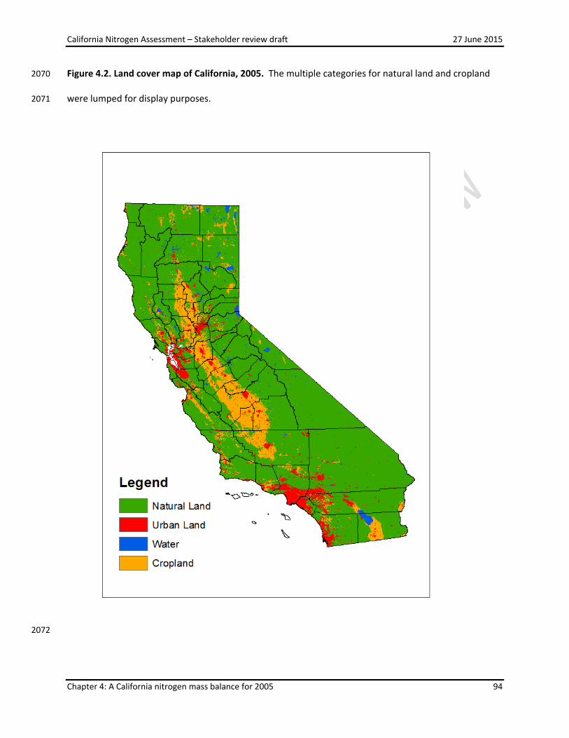
California Nitrogen Assessment – Stakeholder review draft 27 June 2015
Chapter 4: A California nitrogen mass balance for 2005 94
Figure 4.2. Land cover map of California, 2005. The multiple categories for natural land and cropland 2070
were lumped for display purposes. 2071
2072

California Nitrogen Assessment – Stakeholder review draft 27 June 2015
Chapter 4: A California nitrogen mass balance for 2005 95
Figure 4.3 Measuring uncertainty in the California nitrogen mass balance. This figure reflects the amount of evidence and level of agreement 2073
for the various flows of nitrogen covered in the mass balance. Flows represent inputs and outputs as well as transfers of nitrogen within 2074
California. For a more complete catalog of evidence and agreement among data sources, see tables 4.1, 4.2, 4.6, 4.8, 4.9, 4.11, 4.12, 4.14, 4.16, 2075
and the supplemental data tables. 2076
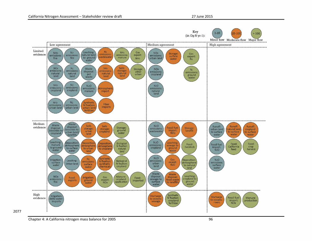
California Nitrogen Assessment – Stakeholder review draft 27 June 2015
Chapter 4: A California nitrogen mass balance for 2005 96
2077

California Nitrogen Assessment – Stakeholder review draft 27 June 2015
Chapter 4: A California nitrogen mass balance for 2005 97
Figure 4.4a. Statewide nitrogen imports to California in 2005 (1617 Gg N yr-1). Synthetic fixation is the 2078
largest single import of N to California contributing 37% of the total. Fossil fuel combustion adds N in 2079
the form of NOx (23%), NH3 (2%), and N2O (1%) to the atmosphere. Biological N fixation is an N input in 2080
both cropland (12%) and natural land (9%). The net import of agricultural products is a source of N in 2081
the form of feed (11%) and fiber (2%). Minor sources of N import are (1) water pumped by the Central 2082
Valley Project and State Water Project in Tracy because it occurs in the Delta downstream of the river 2083
gauges and (2) import of reactive N gases in the atmosphere from across the Pacific Ocean. 2084
2085 2086
2087
2088
2089
2090
2091
2092
2093
2094
2095
2096
2097
2098
2099
2100
36%
22%
12%
12%
9%
3% 2% 2% 1% 1% Synthetic Fixation: 590 Gg
Fossil Fuel Nox: 359 Gg
Feed Imports: 200Gg
Cropland Fixation: 196Gg
Natural Lands Fixation: 139Gg
Fiber Imports: 40Gg
Atmospheric Import: 40Gg
Fossil Fuel NH3: 36Gg
Delta Water Imports: 18Gg

California Nitrogen Assessment – Stakeholder review draft 27 June 2015
Chapter 4: A California nitrogen mass balance for 2005 98
Figure 4.4b. Statewide nitrogen exports, and storage in California in 2005 (1617 Gg N yr-1). The fate of 2101
N imports to California is almost divided between exports (56%) and storage (44%). Atmospheric export 2102
is the dominant fate with NOx (17%), NH3 (13%), N2O (2%), and N2 (13%) accounting for almost half of 2103
the N imports. Nitrogen is exported to the ocean in much smaller amounts from rivers (2%) and as 2104
sewage (5%). The net food balance contributes 5% of the N export. Groundwater (16%) is the single 2105
largest fate as storage with the various other forms of storage in soils and urban environments 2106
combining to account for 28% of the total N import. 2107
2108
2109 2110
2111
2112
17%
16%
13%
13%
8%
6%
5%
5%
4%
4% 4%
2% 2% 1%
NOx : 270 Gg
Groundwater Storage: 257 Gg
N2 : 204 Gg
NH3 : 206 Gg
Other Urban Storage: 123 Gg
Natural Land storage: 91 Gg
Sewage Discharge: 82 Gg
Food: 79 Gg
Urban Land storage: 72 Gg
Landfills storage: 71 Gg
Cropland storage: 67 Gg
River Discharge: 39 Gg
N2O: 38 Gg
Reservoirs storage: 20 Gg

California Nitrogen Assessment – Stakeholder review draft 27 June 2015
Chapter 4: A California nitrogen mass balance for 2005 99
Figure 4.5. Summary of nitrogen imports/inputs (a) and exports/outputs/storage (b) for the three 2113
California land subsystems in 2005. The flows to and from the livestock subsystem (i.e. feed) and the 2114
people/pets subsystem (i.e., food) are shown for comparative purposes, but these subsystems are 2115
calculated independently from the land subsystems. 2116
2117 (a). 2118
2119 2120 (b). 2121
2122
2123
0
200
400
600
800
1000
1200
Cropland Livestock Urban Land People & Pets Natural Land
N fl
ow (G
g N
)
Food Waste Pet Waste
Irrigation Food
Feed Manure
Synthetic Fixation Cropland Fixation
Natural Lands Fixation Deposition
0
200
400
600
800
1000
1200
Cropland Livestock Urban Land People & Pets Natural Land
N fl
ow (G
g N
)
Biosolids Food WastePet Waste FoodFiber FeedManure SewageOther Storage GroundwaterSurface Water FireN2 N2ONH3 NOx

California Nitrogen Assessment – Stakeholder review draft 27 June 2015
Chapter 4: A California nitrogen mass balance for 2005 100
Figure 4.6. Flows of nitrogen in California cropland in 2005. The circled values indicate the absolute 2124
magnitude of the flow in Gg N yr-1 with arrow thickness specifying the relative magnitude of the flow. 2125
Storage terms are indicated with arrows on the circled values. 2126
2127
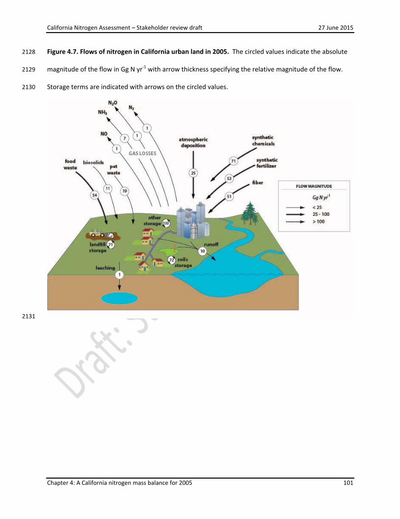
California Nitrogen Assessment – Stakeholder review draft 27 June 2015
Chapter 4: A California nitrogen mass balance for 2005 101
Figure 4.7. Flows of nitrogen in California urban land in 2005. The circled values indicate the absolute 2128
magnitude of the flow in Gg N yr-1 with arrow thickness specifying the relative magnitude of the flow. 2129
Storage terms are indicated with arrows on the circled values. 2130
2131
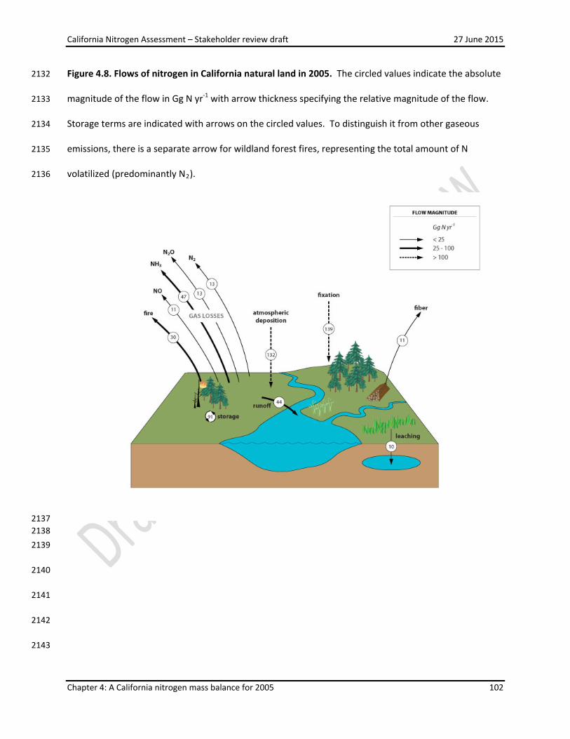
California Nitrogen Assessment – Stakeholder review draft 27 June 2015
Chapter 4: A California nitrogen mass balance for 2005 102
Figure 4.8. Flows of nitrogen in California natural land in 2005. The circled values indicate the absolute 2132
magnitude of the flow in Gg N yr-1 with arrow thickness specifying the relative magnitude of the flow. 2133
Storage terms are indicated with arrows on the circled values. To distinguish it from other gaseous 2134
emissions, there is a separate arrow for wildland forest fires, representing the total amount of N 2135
volatilized (predominantly N2). 2136
2137 2138 2139
2140
2141
2142
2143
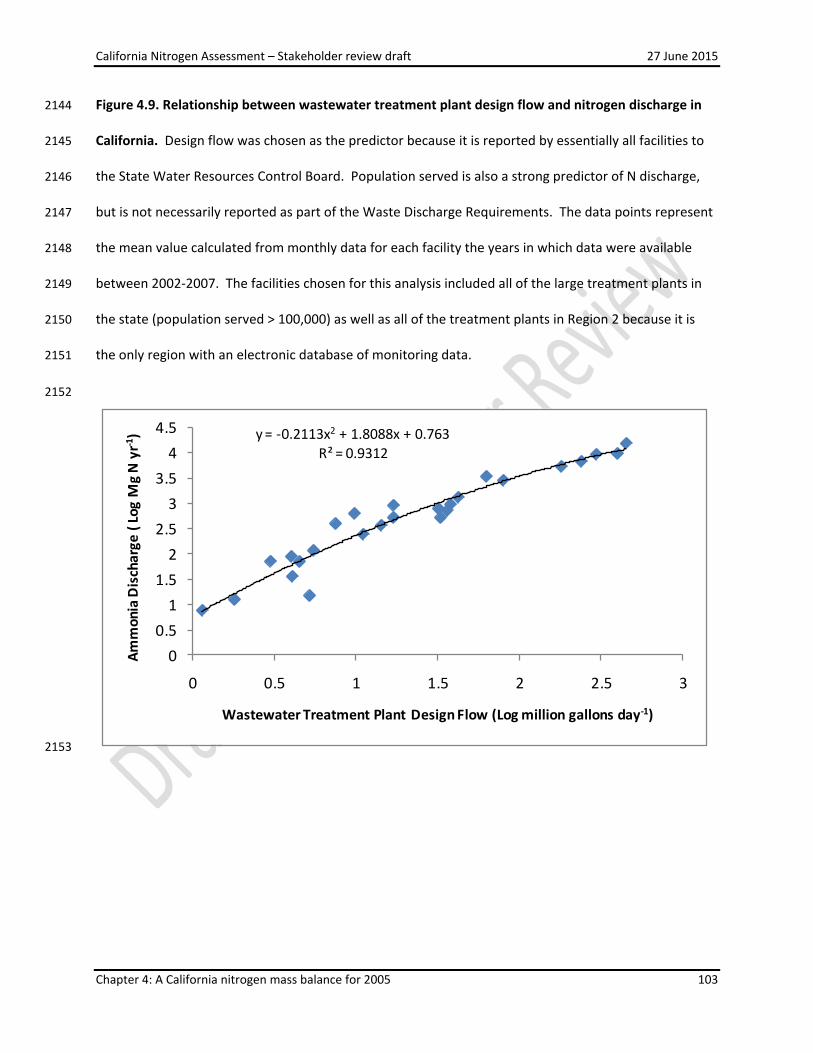
California Nitrogen Assessment – Stakeholder review draft 27 June 2015
Chapter 4: A California nitrogen mass balance for 2005 103
Figure 4.9. Relationship between wastewater treatment plant design flow and nitrogen discharge in 2144
California. Design flow was chosen as the predictor because it is reported by essentially all facilities to 2145
the State Water Resources Control Board. Population served is also a strong predictor of N discharge, 2146
but is not necessarily reported as part of the Waste Discharge Requirements. The data points represent 2147
the mean value calculated from monthly data for each facility the years in which data were available 2148
between 2002-2007. The facilities chosen for this analysis included all of the large treatment plants in 2149
the state (population served > 100,000) as well as all of the treatment plants in Region 2 because it is 2150
the only region with an electronic database of monitoring data. 2151
2152
2153
y = -0.2113x2 + 1.8088x + 0.763R² = 0.9312
00.5
11.5
22.5
33.5
44.5
0 0.5 1 1.5 2 2.5 3
Amm
onia
Dis
char
ge (
Log
Mg
N y
r-1)
Wastewater Treatment Plant Design Flow (Log million gallons day-1)

California Nitrogen Assessment – Stakeholder review draft 27 June 2015
Chapter 4: A California nitrogen mass balance for 2005 104
Figure 4.10. N imports and exports/storage per capita (kg N person-1 yr-1). Comparison of N flows on a 2154
per capita basis for the California N Assessment (CNA) to six representative comprehensive N mass 2155
balance studies at various spatial scales around the world. Data for the Netherlands and Europe are 2156
from Leip et al. (2011), data for the US are from EPA (2011), data for China are from Gu et al. (2009), 2157
data for Korea are from Kim et al. (2008), and data for Phoenix are from Baker et al. (2001). 2158
2159

California Nitrogen Assessment – Stakeholder review draft 27 June 2015
Chapter 4: A California nitrogen mass balance for 2005 105
Figure 4.11. N imports and exports/storage per unit area (kg N ha-1 yr-1). Comparison of N flows on an 2160
areal basis for the California N Assessment (CNA) to six representative comprehensive N mass balance 2161
studies at various spatial scales around the world. Data for the Netherlands and Europe are from Leip et 2162
al. (2011), data for the US are from EPA (2011), data for China are from Gu et al. (2009), data for Korea 2163
are from Kim et al. (2008), and data for Phoenix are from Baker et al. (2001). 2164
2165
2166

California Nitrogen Assessment – Stakeholder review draft 27 June 2015
Chapter 4: A California nitrogen mass balance for 2005 106
Figure 4.12. Relative contribution of N imports and exports/storage. Data for the Netherlands and 2167
Europe are from Leip et al. (2011), data for the US are from EPA (2011), data for China are from Gu et al. 2168
(2009), data for Korea are from Kim et al. (2008), and data for Phoenix are from Baker et al. (2001). 2169
2170
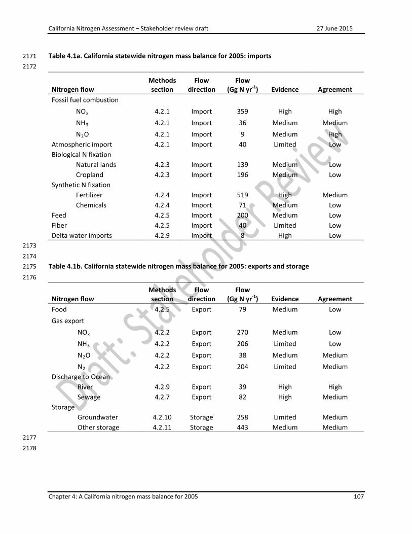
California Nitrogen Assessment – Stakeholder review draft 27 June 2015
Chapter 4: A California nitrogen mass balance for 2005 107
Table 4.1a. California statewide nitrogen mass balance for 2005: imports 2171 2172
Nitrogen flow Methods section
Flow direction
Flow (Gg N yr-1) Evidence Agreement
Fossil fuel combustion
NOx 4.2.1 Import 359 High High
NH3 4.2.1 Import 36 Medium Medium
N2O 4.2.1 Import 9 Medium High
Atmospheric import 4.2.1 Import 40 Limited Low Biological N fixation
Natural lands 4.2.3 Import 139 Medium Low
Cropland 4.2.3 Import 196 Medium Low
Synthetic N fixation
Fertilizer 4.2.4 Import 519 High Medium
Chemicals 4.2.4 Import 71 Medium Low
Feed
4.2.5 Import 200 Medium Low Fiber
4.2.5 Import 40 Limited Low
Delta water imports 4.2.9 Import 8 High Low 2173 2174 Table 4.1b. California statewide nitrogen mass balance for 2005: exports and storage 2175
2176
Nitrogen flow Methods section
Flow direction
Flow (Gg N yr-1) Evidence Agreement
Food
4.2.5 Export 79 Medium Low Gas export
NOx 4.2.2 Export 270 Medium Low
NH3 4.2.2 Export 206 Limited Low
N2O 4.2.2 Export 38 Medium Medium
N2 4.2.2 Export 204 Limited Medium
Discharge to Ocean
River 4.2.9 Export 39 High High
Sewage 4.2.7 Export 82 High Medium
Storage
Groundwater 4.2.10 Storage 258 Limited Medium
Other storage 4.2.11 Storage 443 Medium Medium
2177
2178
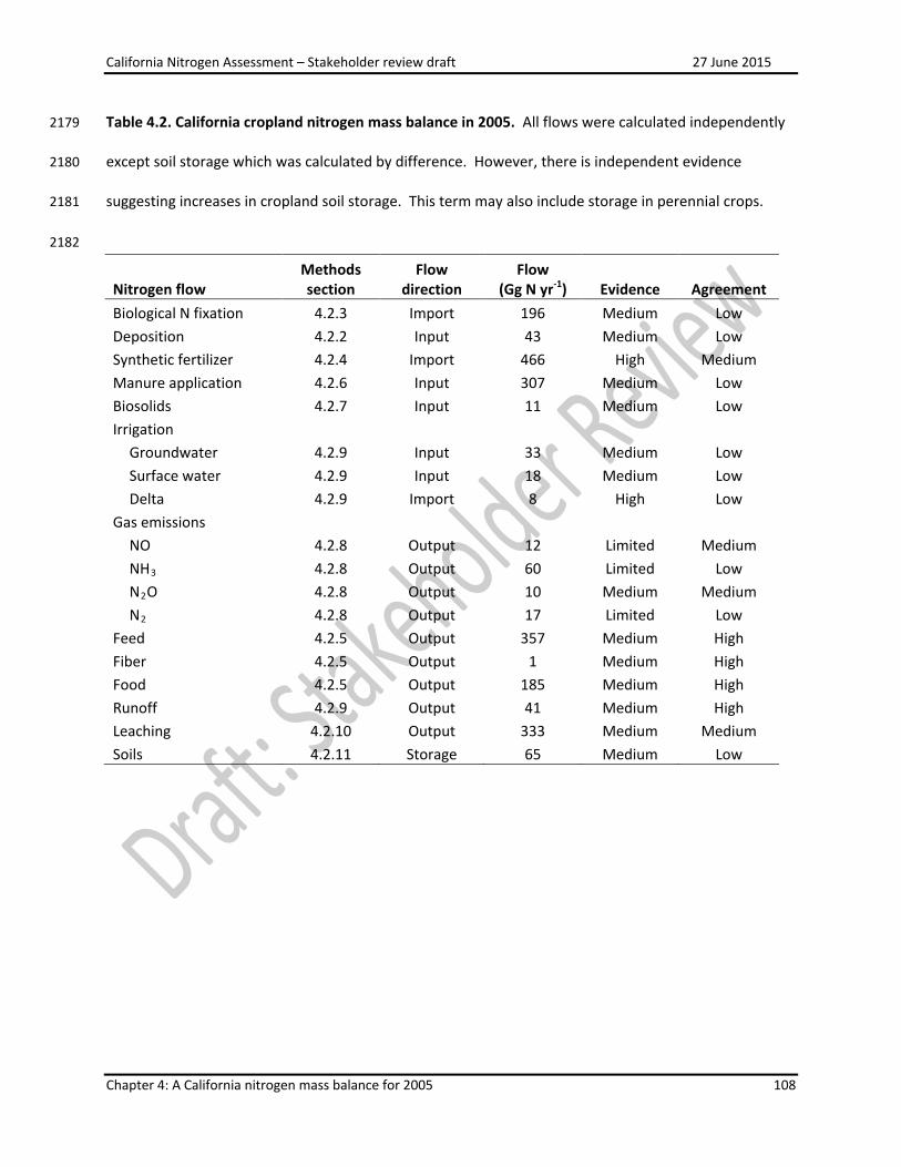
California Nitrogen Assessment – Stakeholder review draft 27 June 2015
Chapter 4: A California nitrogen mass balance for 2005 108
Table 4.2. California cropland nitrogen mass balance in 2005. All flows were calculated independently 2179
except soil storage which was calculated by difference. However, there is independent evidence 2180
suggesting increases in cropland soil storage. This term may also include storage in perennial crops. 2181
2182
Nitrogen flow Methods section
Flow direction
Flow (Gg N yr-1) Evidence Agreement
Biological N fixation 4.2.3 Import 196 Medium Low Deposition 4.2.2 Input 43 Medium Low Synthetic fertilizer 4.2.4 Import 466 High Medium Manure application 4.2.6 Input 307 Medium Low Biosolids 4.2.7 Input 11 Medium Low Irrigation
Groundwater 4.2.9 Input 33 Medium Low
Surface water 4.2.9 Input 18 Medium Low
Delta 4.2.9 Import 8 High Low
Gas emissions
NO 4.2.8 Output 12 Limited Medium
NH3 4.2.8 Output 60 Limited Low
N2O 4.2.8 Output 10 Medium Medium
N2 4.2.8 Output 17 Limited Low
Feed 4.2.5 Output 357 Medium High Fiber 4.2.5 Output 1 Medium High Food 4.2.5 Output 185 Medium High Runoff 4.2.9 Output 41 Medium High Leaching 4.2.10 Output 333 Medium Medium Soils 4.2.11 Storage 65 Medium Low
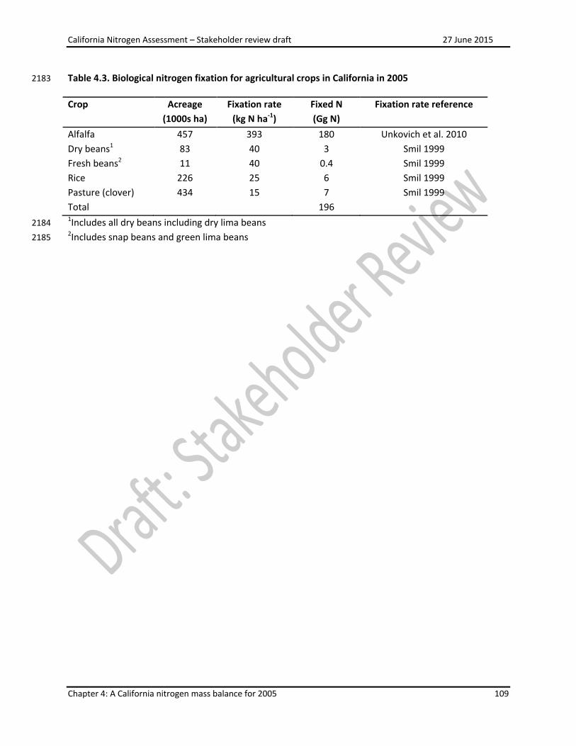
California Nitrogen Assessment – Stakeholder review draft 27 June 2015
Chapter 4: A California nitrogen mass balance for 2005 109
Table 4.3. Biological nitrogen fixation for agricultural crops in California in 2005 2183
Crop Acreage (1000s ha)
Fixation rate (kg N ha-1)
Fixed N (Gg N)
Fixation rate reference
Alfalfa 457 393 180 Unkovich et al. 2010 Dry beans1 83 40 3 Smil 1999 Fresh beans2 11 40 0.4 Smil 1999 Rice 226 25 6 Smil 1999 Pasture (clover) 434 15 7 Smil 1999 Total 196 1Includes all dry beans including dry lima beans 2184 2Includes snap beans and green lima beans 2185
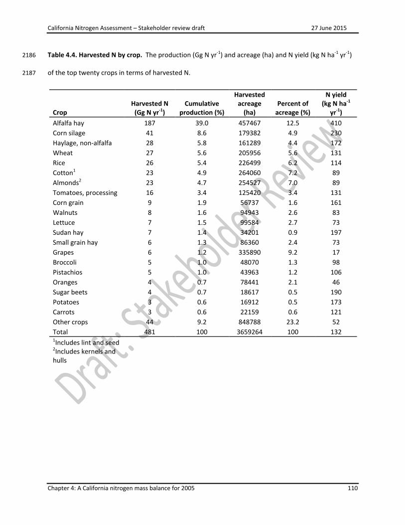
California Nitrogen Assessment – Stakeholder review draft 27 June 2015
Chapter 4: A California nitrogen mass balance for 2005 110
Table 4.4. Harvested N by crop. The production (Gg N yr-1) and acreage (ha) and N yield (kg N ha-1 yr-1) 2186
of the top twenty crops in terms of harvested N. 2187
Crop Harvested N
(Gg N yr-1) Cumulative
production (%)
Harvested acreage
(ha) Percent of
acreage (%)
N yield (kg N ha-1
yr-1) Alfalfa hay 187 39.0 457467 12.5 410 Corn silage 41 8.6 179382 4.9 230 Haylage, non-alfalfa 28 5.8 161289 4.4 172 Wheat 27 5.6 205956 5.6 131 Rice 26 5.4 226499 6.2 114 Cotton1 23 4.9 264060 7.2 89 Almonds2 23 4.7 254527 7.0 89 Tomatoes, processing 16 3.4 125420 3.4 131 Corn grain 9 1.9 56737 1.6 161 Walnuts 8 1.6 94943 2.6 83 Lettuce 7 1.5 99584 2.7 73 Sudan hay 7 1.4 34201 0.9 197 Small grain hay 6 1.3 86360 2.4 73 Grapes 6 1.2 335890 9.2 17 Broccoli 5 1.0 48070 1.3 98 Pistachios 5 1.0 43963 1.2 106 Oranges 4 0.7 78441 2.1 46 Sugar beets 4 0.7 18617 0.5 190 Potatoes 3 0.6 16912 0.5 173 Carrots 3 0.6 22159 0.6 121 Other crops 44 9.2 848788 23.2 52 Total 481 100 3659264 100 132 1Includes lint and seed
2Includes kernels and hulls

California Nitrogen Assessment – Stakeholder review draft 27 June 2015
Chapter 4: A California nitrogen mass balance for 2005 111
Table 4.5. Sources of data for biome-specific NO and N2O fluxes. Biome-specific NO and N2O fluxes 2188
were calculated as the average of several published sources for cropland and natural lands. For the 2189
published studies with areal rates by biome (cropland, desert, coniferous forest, hardwood forest, 2190
grassland, shrubland) we used the biome areas from CAML. For the emissions factor approach we 2191
assumed 1% of fertilizer (both synthetic and manure) were converted to N2O like the California Air 2192
Resources Board. However, we also included a background cropland emission of 1 kg N2O-N ha-1 based 2193
on Stehfest 1996 to calculate total, not just anthropogenic N2O emissions. We also compiled published 2194
estimates of NO and N2O for California cropland. In the case of N2O we used the median flux across all 2195
crops and management practices while for NO we calculated the mean of the daily flux estimates for the 2196
crops measured by Matson et al. (1997). 2197
Source NO (Gg N yr-1)
N2O (Gg N yr-1)
Type of data
Spatial extent
Cropland
Natural land
Cropland
Natural land
Dalal and Allen (2008) 19 Field Global Davidson and Kingerlee (1997) 18 8.9 Field Global Li et al. (1996) 6.9 Model California Potter et al. (1996) 7.4 12 7.9 Model Global Stehfest and Bouwman (2006) 4.9 13 5.9 11
Field Global
Emissions factor 9 Field Global California literature 9 14 Field California
Average estimate 12 11 10 13 2198
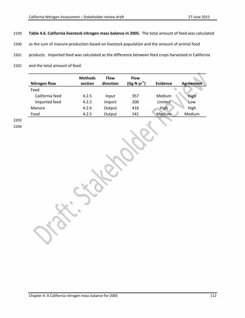
California Nitrogen Assessment – Stakeholder review draft 27 June 2015
Chapter 4: A California nitrogen mass balance for 2005 112
Table 4.6. California livestock nitrogen mass balance in 2005. The total amount of feed was calculated 2199
as the sum of manure production based on livestock population and the amount of animal food 2200
products. Imported feed was calculated as the difference between feed crops harvested in California 2201
and the total amount of feed. 2202
Nitrogen flow Methods section
Flow direction
Flow (Gg N yr-1) Evidence Agreement
Feed
California feed 4.2.5 Input 357 Medium High
Imported feed 4.2.5 Import 200 Limited Low
Manure 4.2.6 Output 416 High High Food 4.2.5 Output 141 Medium Medium
2203
2204

California Nitrogen Assessment – Stakeholder review draft 27 June 2015
Chapter 4: A California nitrogen mass balance for 2005 113
Table 4.7. Confined livestock populations and manure and animal food products in California in 2005. The total N requirement and manure 2205
production are population based estimates based on inventory or sales data. The calculated food produced column is the independent estimate 2206
of food N based on the tonnage of animal food products and their N content. For comparison “Food produced as feed - manure” is calculated as 2207
the difference between the N requirement and manure production. 2208
Class Inventory
(1000 head) Annual sales (1000 head)
Total N requirement
(Gg N)
Manure production
(Gg N)
Calculated food produced
(Gg N)
Food produced as feed - manure
(Gg N) Dairy cow 1,715
351 266 85 86
Dairy heifer 772
42 33 Dairy calf 772
25 18
Layers 21,115
12 6 6 7 Beef steer 644
43 32 18 11
Horses 876
32 35 Turkeys
6,327 4 7 4 -3
Broilers
270,480 35 19 15 15 Pigs
303 3 1 1 2
2209
2210

California Nitrogen Assessment – Stakeholder review draft 27 June 2015
Chapter 4: A California nitrogen mass balance for 2005 114
Table 4.8. Fate of manure nitrogen from confined livestock in California in 2005. Manure production 2211
was calculated based on livestock populations as were ammonia (NH3) emissions. Nitrous oxide (N2O) 2212
emissions were direct emissions from manure prior to land application from the California Air Resources 2213
Board greenhouse gas inventory. All manure except dairy manure was assumed to be utilized as a solid. 2214
Leaching was calculated based on the fraction leached from dairy facilities reported in van der Schans et 2215
al. (2009). 2216
Nitrogen flow Methods section
Flow direction
Flow (Gg N yr-1) Evidence Agreement
Manure production 4.2.6 Input 416 High High Gas emissions
NH3 4.2.6 Output 97 Medium Low
N2O 4.2.6 Output 2 Medium Low
Leaching 4.2.6 Output 10 Medium Low Cropland 4.2.6 Output 307 Medium Low
2217
2218
2219

California Nitrogen Assessment – Stakeholder review draft 27 June 2015
Chapter 4: A California nitrogen mass balance for 2005 115
Table 4.9. California urban land nitrogen mass balance in 2005. All terms except soil storage and other 2220
storage were calculated independently. Soil storage was calculated as the difference between the 2221
inputs of deposition, synthetic fertilizer, and dog waste and the outputs of gases and runoff to surface 2222
water. This storage term may also include storage in perennial vegetation in urban landscapes. Other 2223
storage includes the materials that cannot be tracked to landfills. This includes synthetic chemicals and 2224
some fiber products. 2225
2226
Nitrogen flow Methods section
Flow direction
Flow (Gg N yr-1) Evidence Agreement
Deposition 4.2.2 Input 25 Medium Low Synthetic fertilizer 4.2.4 Import 53 Limited Low Synthetic chemicals 4.2.4 Import 71 Medium Low Fiber 4.2.5 Import 51 Limited Low Food waste to landfill 4.2.7 Input 54 Medium Medium Pet waste 4.2.7 Input 16 Limited Low Biosolids 4.2.7 Input 11 Medium Low Gas emissions
NO 4.2.8 Output 1 Limited Medium
NH3 4.2.8 Output 7 Limited Low
N2O 4.2.8 Output 1 Medium Medium
N2 4.2.8 Output 1 Limited Low
Runoff 4.2.9 Output 10 Medium High Leaching 4.2.10 Output 1 Medium Low Landfill 4.2.7 Storage 71 Medium Medium Soils 4.2.11 Storage 72 Medium Low Other 4.2.11 Storage 122 Limited Low

California Nitrogen Assessment – Stakeholder review draft 27 June 2015
Chapter 4: A California nitrogen mass balance for 2005 116
Table 4.10. Sources of nitrogen to landfills in California in 2005. With the exception of cat waste and 2227
biosolids, which are based on the mass balance, the tonnage of materials sent to the landfill is based on 2228
CIWMB (2004). All moisture and N contents are from Cornell (1992) with the exception of food waste 2229
(Zhang et al. 2007). The category including leaves and grass was assumed to be equally composed of 2230
these two materials. Only food waste and cat waste are considered a new input to urban land while the 2231
other organic materials were already considered part of the urban landscape. 2232
Material Tonnes Moisture (%) N (%) Gg N Paper 7,678,172 20 0.1 6.1 Lumber 3,528,376 15 0.1 3.0 Prunings 836,687 15 0.1 0.7 Stumps 108,867 15 0.1 0.1 Food 5,322,138 74 3.2 44.3 Leaves and grass 1,541,838
9.0
Manure 33,187 72 1.6 0.1 Cat waste
3
Biosolids
11 Total
68
2233
2234
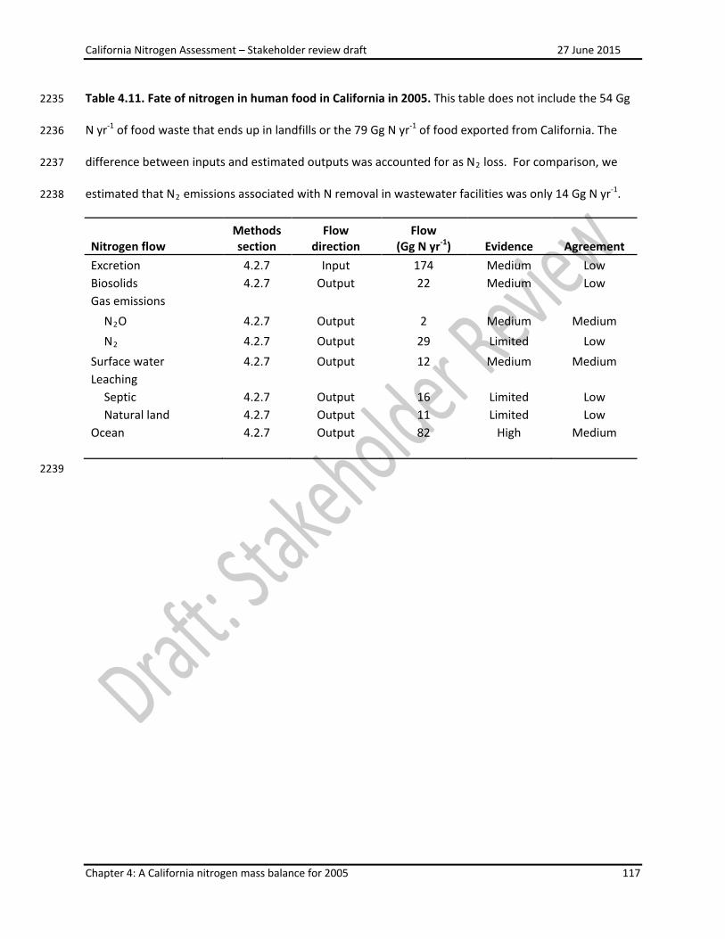
California Nitrogen Assessment – Stakeholder review draft 27 June 2015
Chapter 4: A California nitrogen mass balance for 2005 117
Table 4.11. Fate of nitrogen in human food in California in 2005. This table does not include the 54 Gg 2235
N yr-1 of food waste that ends up in landfills or the 79 Gg N yr-1 of food exported from California. The 2236
difference between inputs and estimated outputs was accounted for as N2 loss. For comparison, we 2237
estimated that N2 emissions associated with N removal in wastewater facilities was only 14 Gg N yr-1. 2238
Nitrogen flow Methods section
Flow direction
Flow (Gg N yr-1) Evidence Agreement
Excretion 4.2.7 Input 174 Medium Low Biosolids 4.2.7 Output 22 Medium Low Gas emissions
N2O 4.2.7 Output 2 Medium Medium
N2 4.2.7 Output 29 Limited Low
Surface water 4.2.7 Output 12 Medium Medium Leaching
Septic 4.2.7 Output 16 Limited Low
Natural land 4.2.7 Output 11 Limited Low
Ocean 4.2.7 Output 82 High Medium
2239

California Nitrogen Assessment – Stakeholder review draft 27 June 2015
Chapter 4: A California nitrogen mass balance for 2005 118
Table 4.12. California natural land nitrogen mass balance in 2005. Storage was estimated as the 2240
difference between inputs and outputs and could occur in soils or vegetation. 2241
Nitrogen flow Methods section
Flow direction
Flow (Gg N yr-1) Evidence Agreement
Biological N fixation 4.2.3 Import 139 Medium Low Deposition 4.2.2 Input 132 Medium Medium Gas emissions
NO 4.2.8 Output 11 Limited Low
NH3 4.2.8 Output 47 Limited Low
N2O 4.2.8 Output 13 Limited Medium
N2 4.2.8 Output 13 Limited Low
Fire 4.2.8 Output 30 Limited Low
Runoff 4.2.9 Output 44 Medium High Leaching 4.2.10 Output 10 Limited Low Fiber 4.2.5 Output 11 Limited Low Storage 4.2.11 Storage 91 Limited Low
2242

California Nitrogen Assessment – Stakeholder review draft 27 June 2015
Chapter 4: A California nitrogen mass balance for 2005 119
Table 4.13. Atmospheric nitrogen balance for California in 2005. Only the fossil fuel combustion and the upwind sources of N were new 2243
statewide inputs of N. All N2 and N2O emitted were assumed to be an output from the state. For NOx and NH3, export beyond the state 2244
boundary of these gases was calculated as the difference between emissions and deposition. Because of reactions in the atmosphere, a 2245
significant fraction of the export of oxidized and reduced N has been converted to chemical forms (e.g., nitric acid, ammonium nitrate particles, 2246
peroxyacetyl nitrate) other than NOx and NH3. These oxidized and reduced forms are often summarized as NOy and NHx. 2247
N flow Methods section
Flow direction
NOx (Gg N yr-1)
NH3 (Gg N yr-1)
N2O (Gg N yr-1)
N2 (Gg N yr-1)
Total (Gg N yr-1)
Fossil fuel combustion 4.2.1 Import 359 36 9
404 Soil 4.2.8 Input 24 110 24 31 188 Manure 4.2.6 Input
97 2
99
Upwind sources 4.2.1 Import 20 20
40 Wastewater 4.2.7 Input
2 29 31
Pet Waste 4.2.7 Input 4 4 Fire 4.2.8 Input 3 3
24 30
Surface water 4.2.9 Input
2 34 31 Groundwater 4.2.10 Input 91 91 Deposition 4.2.2 Output 135 67
202
Export 4.2.2 Export 270 203 38 204 716 2248
2249
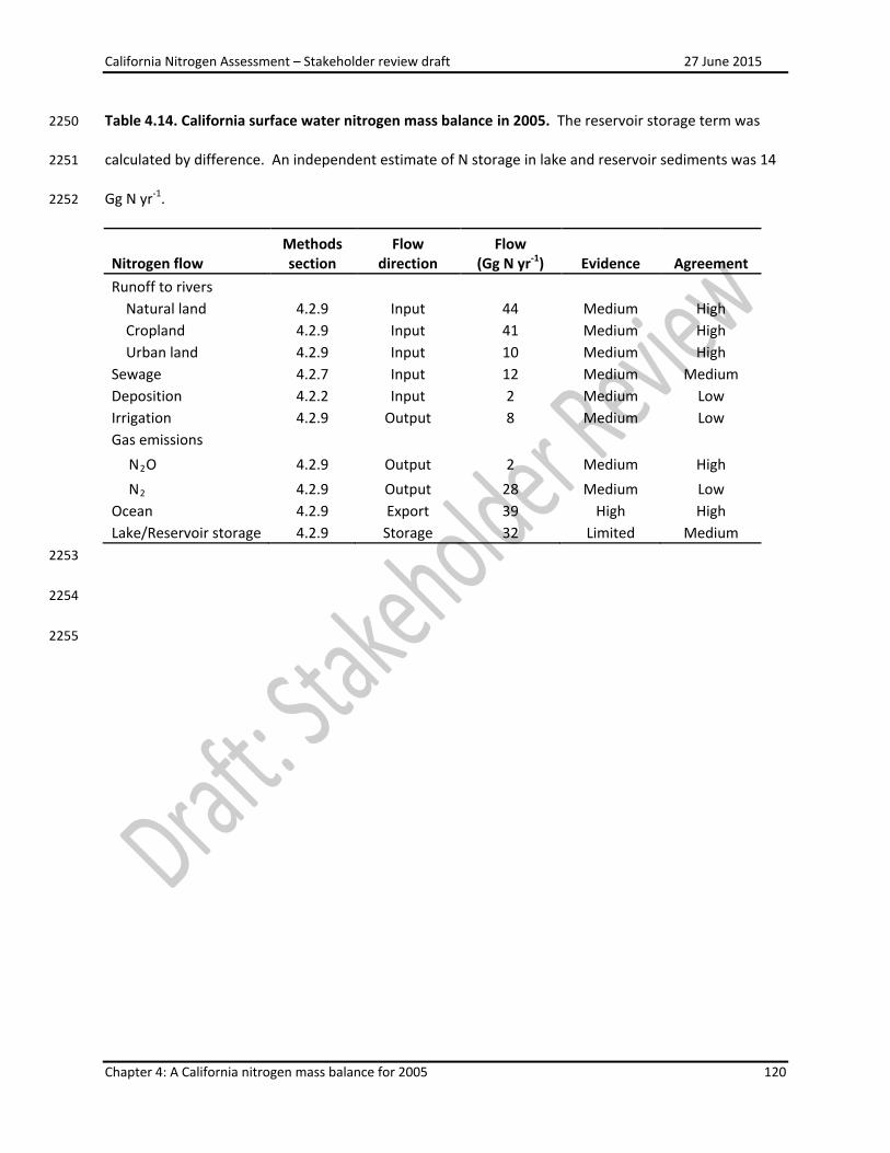
California Nitrogen Assessment – Stakeholder review draft 27 June 2015
Chapter 4: A California nitrogen mass balance for 2005 120
Table 4.14. California surface water nitrogen mass balance in 2005. The reservoir storage term was 2250
calculated by difference. An independent estimate of N storage in lake and reservoir sediments was 14 2251
Gg N yr-1. 2252
2253
2254
2255
Nitrogen flow Methods section
Flow direction
Flow (Gg N yr-1) Evidence Agreement
Runoff to rivers Natural land 4.2.9 Input 44 Medium High
Cropland 4.2.9 Input 41 Medium High Urban land 4.2.9 Input 10 Medium High Sewage 4.2.7 Input 12 Medium Medium Deposition 4.2.2 Input 2 Medium Low Irrigation 4.2.9 Output 8 Medium Low Gas emissions
N2O 4.2.9 Output 2 Medium High
N2 4.2.9 Output 28 Medium Low
Ocean 4.2.9 Export 39 High High Lake/Reservoir storage 4.2.9 Storage 32 Limited Medium
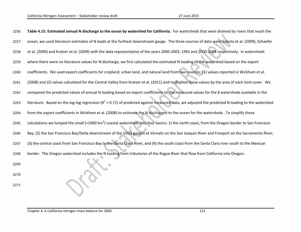
California Nitrogen Assessment – Stakeholder review draft 27 June 2015
Chapter 4: A California nitrogen mass balance for 2005 121
Table 4.15. Estimated annual N discharge to the ocean by watershed for California. For watersheds that were drained by rivers that reach the 2256
ocean, we used literature estimates of N loads at the furthest downstream gauge. The three sources of data were Sobota et al. (2009), Schaefer 2257
et al. (2009) and Kratzer et al. (2009) with the data representative of the years 2000-2003, 1992 and 2000-2004 respectively. In watersheds 2258
where there were no literature values for N discharge, we first calculated the estimated N loading to the watershed based on the export 2259
coefficients. We used export coefficients for cropland, urban land, and natural land from two sources: (1) values reported in Wickham et al. 2260
(2008) and (2) values calculated for the Central Valley from Kratzer et al. (2011) and multiplied these values by the area of each land cover. We 2261
compared the predicted values of annual N loading based on export coefficients to the measured values for the 8 watersheds available in the 2262
literature. Based on the log-log regression (R2 = 0.71) of predicted against measured data, we adjusted the predicted N loading to the watershed 2263
from the export coefficients in Wickham et al. (2008) to estimate the N discharged to the ocean for the watersheds . To simplify these 2264
calculations we lumped the small (<1000 km2) coastal watersheds into four basins: 1) the north coast, from the Oregon border to San Francisco 2265
Bay, (2) the San Francisco Bay/Delta downstream of the USGS gauges at Vernalis on the San Joaquin River and Freeport on the Sacramento River, 2266
(3) the central coast from San Francisco Bay to the Santa Clara River, and (4) the south coast from the Santa Clara river south to the Mexican 2267
border. The Oregon watershed includes the N loading from tributaries of the Rogue River that flow from California into Oregon. 2268
2269
2270
2271
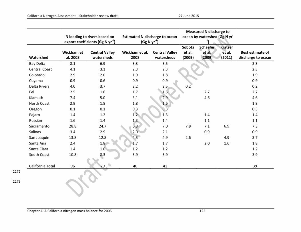
California Nitrogen Assessment – Stakeholder review draft 27 June 2015
Chapter 4: A California nitrogen mass balance for 2005 122
N loading to rivers based on export coefficients (Gg N yr-1)
Estimated N discharge to ocean (Gg N yr-1)
Measured N discharge to ocean by watershed (Gg N yr-
1)
Watershed Wickham et
al. 2008 Central Valley
watersheds Wickham et al.
2008 Central Valley
watersheds
Sobota et al.
(2009)
Schaefer et al.
(2009)
Kratzer et al.
(2011) Best estimate of
discharge to ocean Bay Delta 8.1 6.9 3.3 3.5
3.3
Central Coast 4.1 3.1 2.3 2.3
2.3 Colorado 2.9 2.0 1.9 1.8
1.9
Cuyama 0.9 0.6 0.9 0.9
0.9 Delta Rivers 4.0 3.7 2.2 2.5 0.2
0.2
Eel 2.5 1.6 1.7 1.5
2.7
2.7 Klamath 7.4 5.0 3.1 2.9
4.6
4.6
North Coast 2.9 1.8 1.8 1.6
1.8 Oregon 0.1 0.1 0.3 0.3
0.3
Pajaro 1.4 1.2 1.2 1.3
1.4
1.4 Russian 1.6 1.4 1.3 1.4
1.1
1.1
Sacramento 28.8 24.7 6.8 7.0 7.8 7.1 6.9 7.3 Salinas 3.4 2.9 2.0 2.1
0.9
0.9
San Joaquin 13.8 12.8 4.5 4.9 2.6
4.9 3.7 Santa Ana 2.4 1.8 1.7 1.7
2.0 1.6 1.8
Santa Clara 1.4 1.0 1.2 1.2
1.2 South Coast 10.8 8.3 3.9 3.9
3.9
California Total 96 79 40 41
39 2272
2273

California Nitrogen Assessment – Stakeholder review draft 27 June 2015
Chapter 4: A California nitrogen mass balance for 2005 123
Table 4.16. California groundwater nitrogen flows in 2005. We assumed no net transport of N between 2274
surface water and groundwater. Storage of N in groundwater was calculated as the difference between 2275
inputs and outputs. 2276
Nitrogen flow Methods section
Flow direction
Flow (Gg N yr-1) Evidence Agreement
Soils leaching
Cropland 4.2.10 Input 333 Medium High
Urban land 4.2.10 Input 1 Medium Low
Natural land 4.2.10 Input 10 Limited Low
Manure leaching 4.2.6 Input 10 Medium Low Sewage leaching 4.2.7 Input 27 Medium Medium
Irrigation 4.2.10 Output 33 Medium Low Denitrification 4.2.10 Output 91 Limited Medium Storage 4.2.10 Storage 258 Medium Low
2277
2278
California Nitrogen Assessment – Stakeholder review draft 27 June 2015
Chapter 4: A California nitrogen mass balance for 2005 124
Table 4.17. Major non-fertilizer uses of synthetic nitrogen in the United States. Source: Domene and 2279
Ayres 2001. 2280
Compound N (Gg yr-1) End use Acrylonitrile 173 Acrylonitrile Butadiene Styrene Caprolactam 86 Nylon Hexamethylenediamine 203 Nylon Isocyanates 90 Polyurethane Melamine 54 Laminates and surface coatings Urea 180 Resins Adipic Acid1 185 Nylon Manufacturing Methylmethylacrylate2 102 Acrylic glass manufacturing 2281 1NOx, N2O, and N2 emissions from the reduction of nitric acid are a byproduct of adipic acid synthesis, 2282
but N is not a component of the product. 2283
2Ammonium sulfate, typically used as fertilizer, is produced as a byproduct of methylmethylacrylate 2284 synthesis. 2285
2286
California Nitrogen Assessment – Stakeholder review draft 27 June 2015
Chapter 4: A California nitrogen mass balance for 2005 125
Table 4.18. Synthetic nitrogen consumption (Gg N yr-1) in the United States. Where possible, non-2287
fertilizer consumption was partitioned into explosives, plastics and synthetics, and other uses. 2288
Source Year Fertilizer Non-fertilizer
Explosives Plastics and synthetics
Other
Kramer 2004 2002 11,636 1,565 998 491 76 FAO (2013) 2002 10,945 4,277 Domene and Ayres 2001 1996 11,297 3,020 557 786 1677 2289 2290

California Nitrogen Assessment – Stakeholder review draft 27 June 2015
Chapter 4: A California nitrogen mass balance for 2005 126
Table 4.19. Assumed nitrogen content of animal products. Source: NRC 2003. 2291
Product N content (%)
Hogs, beef 2 Milk 0.5 Eggs 1.8 Broilers, turkeys 2.3
2292

California Nitrogen Assessment – Stakeholder review draft 27 June 2015
Chapter 4: A California nitrogen mass balance for 2005 127
Table 4.20. References for other nitrogen mass balance studies. Types of mass balances include the 2293
Net Anthropogenic Nitrogen Inputs (NANI) approach described by Jordan and Weller (1996), 2294
comprehensive approaches that include all N flows, and intermediate approaches that examine only a 2295
subset of the landscape (e.g., agriculture) or a subset of the flows across the entire landscape. 2296
Author Year Type Spatial Extent Antikainen 2005 Comprehensive Country Baisre 2006 NANI Country Baker 2001 Comprehensive Region Bormann 1977 NANI Watershed Boyer 2002 NANI Watersheds Carey 2001 NANI Watersheds Castro 2003 NANI Watersheds David 2000 NANI State Delwiche 1970 Intermediate Global EPA 2011 Intermediate Country Galloway 2004 Intermediate Global/Continents Goolsby 1999 Intermediate Watershed Gu 2009 Comprehensive Region Han 2011 NANI Region Han 2008 NANI Watersheds Howarth 1996 NANI Watersheds Howarth 2012 NANI Watersheds Janzen 2003 Agriculture Country Jordan 1996 NANI Watersheds Keeney 1979 Intermediate State Kim 2008 Comprehensive Country Leip 2011 Comprehensive Country Messer 1983 Agriculture State Miller 1976 Agriculture Region NRC 1972 Intermediate Country OECD 2001 Agriculture Country Parfitt 2006 Intermediate Country Prasad 2004 Agriculture Country Quynh 2005 Intermediate Watersheds Robertson 1986 Intermediate Countries Salo 2007 Agriculture Country Schaefer 2007 NANI Watersheds Schaefer 2009 NANI Watersheds Sobota 2009 NANI Watersheds
California Nitrogen Assessment – Stakeholder review draft 27 June 2015
Chapter 4: A California nitrogen mass balance for 2005 128
Soderlund 1976 Intermediate Global Valiela 2002 NANI Watersheds van Drecht 2003 Intermediate Global Velmuragan 2008 Intermediate Country
2297
2298