Chapter 3

Statistics for Describing, Exploring, and Comparing Data

3-2 Measures of Center 1. The mean, median, mode, and midrange are measures of “center” in the sense that they each attempt to determine (by various criteria – i.e., by using different approaches) what might be designated as a typical or representative value.

2. The term “average” is not used in statistics because it is imprecisely used by the general public as a synonym for “typical” – as in, the average American has blue eyes. When referring to the result obtained by dividing a sum by the number of values contributing to that sum, the term “mean” should be used.

3. No. The price “exactly in between the highest and the lowest” would be the mean of the highest and lowest values – which is the midrange, and not the median.

4. No. Since the numbers are not measuring anything, their mean would be meaningless. In general, the mean is not meaningful or appropriate when there are no units (e.g., pounds, inches, etc.) associated with the values.

NOTE: As it is common in mathematics and statistics to use symbols instead of words to represent quantities that are used often and/or that may appear in equations, this manual employs the following symbols for the various measures of center. mean = x mode = M median = x̃ midrange = m.r. This manual will generally report means, medians and midranges accurate to one more decimal place than found in the original data. In addition, these two conventions will be employed.

(1) When there is an odd number of data, the median will be one of the original values. The manual follows example #2 in this section and reports the median as given in the original data. And so the median of 1,2,3,4,5 is reported as x̃ = 3.

(2) When the mean falls exactly between two values accurate to one more decimal place than the original data, the round-off rule in this section gives no specific direction. This manual follows the commonly accepted convention of always rounding up. And so the mean of 1,2,3,3 is reported as x = 9/4 = 2.3 [i.e., 9/4 = 2.25, rounded up to 2.3].

In addition, the median is the middle score when the scores are arranged in order, and the midrange is halfway between the first and last score when the scores are arranged in order. It is usually helpful to arrange the scores in order. This will not affect the mean, and it may also help in identifying the mode. Finally, no measure of center can have a value lower than the smallest score or higher than the largest score. Remembering this helps to protect against gross errors, which most commonly occur when calculating the mean.

5. Arranged in order, the n=10 scores are: 34 36 39 43 51 53 62 63 73 79 a. x = (Σx)/n = (533)/10 = 53.3 words c. M = (none) b. x = (51 + 53)/2 = 52.0 words d. m.r. = (34 + 79)/2 = 56.5 words Using the mean of 53.3 words per page, a reasonable estimate for the total number of words in the dictionary is (53.3)(1459) = 77,765. Since the sample is a simple random sample, it should be representative of the population and the estimate of 77,675 is a valid estimate for the number of words in the dictionary – but not for the total number of words in the English

Measures of Center SECTION 3.2 45 language, since the dictionary does not claim to contain every word. NOTE: The exercise also asks whether the estimate for the total is “accurate.” This is a relative term. A change of 1.0 in the estimate for the mean produces a change of 1459 in the estimate for the total. While a change of 1459 is only a change of 1459/77765 = 1.9%, this illustrates that accuracy in terms of absolute numbers is sometimes hard to attain when estimating totals.

6. Arranged in order, the n=6 scores are: 431 546 612 649 774 1210 a. x = (Σx)/n = (4222)/6 = 703.7 hic c. M = (none) b. x = (612 + 649)/2 = 630.5 hic d. m.r. = (431 + 1210)/2 = 820.5 hic No. Even though all four measures of center fall within with accepted guidelines, all the individual values do not. Since one result exceeds the guidelines, it is clear that all child booster seats do not meet the requirement. NOTE: Even for a very large sample (e.g., n=10,000), if one sample value exceeds the guidelines then it is clear that all the seats in the population do not meet the requirement. For the given sample of size n=6, a sample failure rate of 1/6 = 17% suggests a population failure rate too large to ignore. For a sample of size n=10,000, a sample failure rate of 1/10,000 = 0.01% would likely be acceptable – even though all seats still do not meet the requirement.

7. Arranged in order, the n=5 scores are: 4277 4911 6374 7448 9051 a. x = (Σx)/n = (32061)/5 = $6412.2 c. M = (none) b. x = $6374 d. m.r. = (4277 + 9051)/2 = $6664.0 No. Even though the sample values cover a fairly wide range, the measures of center do not differ very much.

8. Arranged in order, the n=12 scores are: 664 693 698 714 751 753 779 789 802 818 834 836 a. x = (Σx)/n = (9131)/12 = 760.9 points c. M = (none) b. x = (753 + 779)/2 = 766.0 points d. m.r. = (664 + 836)/2 = 750.0 points No. The sample mean of 760.9 appears to be significantly higher than the reported mean, and 11 of the 12 values are higher than the reported mean. The sample FICO scores do not appear to be consistent with the reported mean.

9. Arranged in order, the n=10 scores are: 8.4 9.6 10 12 13 15 27 35 36 38 a. x = (Σx)/n = (204)/10 = $20.4 million c. M = (none) b. x = (13 + 15)/2 = $14.0 million d. m.r. = (8.4 + 38)/2 = $23.2 million No, the top ten salaries provide no information (other than an upper cap) about the salaries of TV personalities in general. No, top 10 lists are generally not valuable for gaining insight into the larger population. NOTE: The “one more decimal place than is present in the original set of values” round-off rule given in the text sometimes requires thought before being applied. Since the data in this exercise is presented with two digit accuracy, the rule suggests reporting the appropriate measures of center with three digit accuracy.

10. Arranged in order, the n=25 scores are: 1 1 1 1 1 1 1 1 1 1 1 2 2 2 2 2 2 2 3 3 3 3 3 3 4 a. x = (Σx)/n = (47)/25 = 1.9 c. M = 1 b. x = 2 d. m.r. = (1 + 4)/2 = 2.5 Yes, the measures of center can be calculated. No, the measures of center do not make any sense – except for the mode of 1, which indicates that the smooth-yellow phenotype occurs more than any of the others. Re-numbering the phenotypes would not actually change the results, but it would give different numerical values to the calculated measures.

46 CHAPTER 3 Statistics for Describing, Exploring, and Comparing Data 11. Arranged in order, the n=15 scores are: 0 73 95 165 191 192 221 235 235 244 259 262 331 376 381 a. x = (Σx)/n = (3260)/15 = 217.3 hrs c. M = 235 hrs b. x = 235 hrs d. m.r. = (0 + 381)/2 = 190.5 hrs The duration time of 0 appears to be very unusual. It likely represents the Challenger disaster of January 1986, when the mission ended in an explosion shortly after takeoff.

12. Arranged in order, the n=18 scores are: −5 −2 −2 −2 −2 0 0 1 1 2 2 3 3 4 5 7 8 11 a. x = (Σx)/n = (34)/18 = 1.9 kg c. M = −2 kg b. x = (1 + 2)/2 = 1.5 kg d. m.r. = (−5 + 11)/2 = 3.0 kg No, these data do not appear to support the legendary 6.8 kg figure. All of the measures of center are well below 6.8, as are 15/18 = 83.3% of the sample values.

13. Arranged in order, the n=20 scores are: 1 2 2 2 2 2 2 2 2 2 2 2 2 2 3 3 3 3 4 4 a. x = (Σx)/n = (47)/20 = 2.4 mpg c. M = 2 mpg b. x = (2 + 2)/2 = 2.0 mpg d. m.r. = (1 + 4)/2 = 2.5 mpg No, there would not be much of an error. Since the amounts do not vary much, the mean appears to be a reasonable value to use for each of the older cars.

14. Arranged in order, the n=8 scores are: 150,000 229,000 232,425 300,000 350,147 360,000 810,000 1,231,421 a. x = (Σx)/n = (3,662,993)/8 = $457,874.1 c. M = (none) b. x = (300,000 + 350,147)/2 = $325,073.5 d. m.r. = (150,000 + 1,231,421)/2 = $690,710.5 If the highest salary is omitted the mean changes to (2,431,572)/7 = $347,367.4 and the median changes to $300,000. Both measures decrease, but the mean decreases by a larger amount.

15. Arranged in order, the n=16 scores are: 213 213 227 231 239 242 244 246 246 255 257 258 262 280 293 448 a. x = (Σx)/n = (4154)/16 = 259.6 sec c. M = 213 sec, 246 sec (bimodal) b. x = (246 + 246)/2 = 246.0 sec d. m.r. = (213 + 448)/2 = 330.5 sec Yes, the time of 448 seconds appears to be very different from the others.

16. Arranged in order, the n=24 scores are: 1 1 1 1 1 1 1 1 1 1 2 2 3 3 3 4 4 5 7 8 15 17 18 158 a. x = (Σx)/n = (259)/24 = 10.8 satellites c. M = 1 satellite b. x = (2 + 3)/2 = 2.5 satellites d. m.r. = (1 + 158)/2 = 79.5 satellites Yes, the country with 158 satellites has an exceptional number of them. That country is most likely the United States.

17. Arranged in order, the n=20 scores are: 4 4 4 4 4 4 4.5 4.5 4.5 4.5 4.5 4.5 6 6 8 9 9 13 13 15 a. x = (Σx)/n = (130)/20 = 6.5 yrs c. M = 4 yrs, 4.5 yrs (bi-modal) b. x = (4.5 + 4.5)/2 = 4.5 yrs d. m.r. = (4 + 14)/2 = 9.5 yrs Yes, it is common to earn a bachelor’s degree in 4 years in that we estimate that 6/20 = 30% of the people do so – but the typical time to earn a bachelor’s degree appears to be more than that. NOTE: The “one more decimal place than is present in the original set of values” round-off rule given in the text sometimes requires thought before being applied. In this exercise it appears that the basic measurement is being done in whole number of years, and so the appropriate measures of center should be reported with one decimal accuracy. When there are different number of decimal places in the original data, it is generally appropriate to use the least accurate data as the basis for applying the round-off rule.

Measures of Center SECTION 3.2 47 18. Arranged in order, the n=8 scores are: 6.5 7.1 7.2 7.2 7.4 7.9 8.2 9.3 a. x = (Σx)/n = (60.8)/8 = 7.60 tons c. M = 7.2 tons b. x = (7.2 + 7.4)/2 = 7.30 tons d. m.r. = (6.5 + 9.3)/2 = 7.90 tons No, in a simple random sample all possible samples of size n are equally likely. Since Data Set 16 does not include every model of cars in use in the population, it cannot produce a simple random sample of the population.

19. Arranged in order, the n=12 scores are: 14 15 59 85 95 97 98 106 117 120 143 371 a. x = (Σx)/n = (1320)/12 = 110.0 c. M = (none) b. x = (97 + 98)/2 = 97.5 d. m.r. = (14 + 371)/2 = 192.5 Yes, there does appear to be a trend in the data. The numbers of bankruptcies seems to steadily increase up to a certain point and then drop off dramatically. It could be that new bankruptcy laws (that made it more difficult to declare bankruptcy) went into effect.

20. Arranged in order, the n=40 scores are: 114 116 128 129 130 133 136 137 138 140 142 142 144 145 145 145 147 149 150 150 150 151 151 151 151 152 155 156 156 158 158 161 163 163 165 166 169 170 172 188 a. x = (Σx)/n = (5966)/40 = 149.2 mBq c. M = 151 mBq b. x = (150 + 150)/2 = 150.0 mBq d. m.r. = (114 + 188)/2 = 151.0 mBq The measures of center are close to each other, suggesting a nearly symmetric distribution.

21. Arranged in order, the scores are as follows. 30 days: 244 260 264 264 278 280 318 one day: 456 536 567 614 628 943 1088 30 days one day n = 7 n = 7 x = (Σx)/n = 1908/7 = $272.6 x = (Σx)/n = 4832/7 = $690.3 x = $264 x = $614 The tickets purchased 30 days in advance are considerably less expensive – they appear to cost less than half of the tickets purchased one day in advance.

22. Arranged in order, the scores are as follows. former: 18.4 18.8 18.9 19.1 19.4 20.3 20.4 21.9 22.1 22.3 recent: 16.8 17.6 17.8 17.9 18.8 19.1 19.5 19.6 20.2 20.3 former recent n = 10 n = 10 x = (Σx)/n = 201.6/10 = 20.16 x = (Σx)/n = 187.6/10 = 18.76 x = (19.4 + 20.3)/2 = 19.85 x = (18.8 + 19.1)/2 = 18.95 The recent winners appear to have lower measures of BMI than do the former winners.

23. Arranged in order, the scores are as follows. non-filtered: 1.0 1.1 1.1 1.1 1.1 1.1 1.1 1.1 1.1 1.1 1.1 1.1 1.1 1.1 1.2 1.2 1.3 1.3 1.4 1.4 1.5 1.6 1.7 1.7 1.8 filtered: 0.2 0.4 0.6 0.8 0.8 0.8 0.8 0.8 0.8 0.8 0.9 1.0 1.0 1.0 1.0 1.0 1.1 1.1 1.1 1.1 1.1 1.1 1.1 1.2 1.3 non-filtered filtered n = 25 n = 25 x = (Σx)/n = 31.4/25 = 1.26 mg x = (Σx)/n = 22.9/25 = 0.92 mg x = 1.1mg x = 1.0 mg The filtered cigarettes seem to have less nicotine. Filters appear to be effective in reducing the amounts of nicotine.

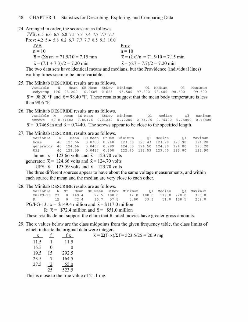
48 CHAPTER 3 Statistics for Describing, Exploring, and Comparing Data 24. Arranged in order, the scores are as follows. JVB: 6.5 6.6 6.7 6.8 7.1 7.3 7.4 7.7 7.7 7.7 Prov: 4.2 5.4 5.8 6.2 6.7 7.7 7.7 8.5 9.3 10.0 JVB Prov n = 10 n = 10 x = (Σx)/n = 71.5/10 = 7.15 min x = (Σx)/n = 71.5/10 = 7.15 min x = (7.1 + 7.3) /2 = 7.20 min x = (6.7 + 7.7)/2 = 7.20 min The two data sets have identical means and medians, but the Providence (individual lines) waiting times seem to be more variable.

25. The Minitab DESCRIBE results are as follows. Variable N Mean SE Mean StDev Minimum Q1 Median Q3 Maximum BodyTemp 106 98.200 0.0605 0.623 96.500 97.800 98.400 98.600 99.600

x = 98.20 °F and x = 98.40 °F. These results suggest that the mean body temperature is less than 98.6 °F.

26. The Minitab DESCRIBE results are as follows. Variable N Mean SE Mean StDev Minimum Q1 Median Q3 Maximum screws 50 0.74682 0.00174 0.01232 0.72200 0.73775 0.74400 0.75800 0.76800

x = 0.7468 in and x = 0.7440. The screws appear to be close to the specified length.

27. The Minitab DESCRIBE results are as follows. Variable N Mean SE Mean StDev Minimum Q1 Median Q3 Maximum home 40 123.66 0.0380 0.240 123.30 123.43 123.70 123.90 124.20 generator 40 124.66 0.0457 0.289 124.00 124.50 124.70 124.80 125.20 UPS 40 123.59 0.0487 0.308 122.90 123.53 123.70 123.80 123.90

home: x = 123.66 volts and x = 123.70 volts generator: x = 124.66 volts and x = 124.70 volts UPS: x = 123.59 volts and x = 123.70 volts The three different sources appear to have about the same voltage measurements, and within each source the mean and the median are very close to each other.

28. The Minitab DESCRIBE results are as follows. Variable N N* Mean SE Mean StDev Minimum Q1 Median Q3 Maximum PG/PG-13 23 0 149.4 22.5 108.0 12.0 100.0 117.0 228.0 380.0 R 12 0 72.4 16.7 57.8 5.00 33.3 51.0 108.5 209.0

PG/PG-13: x = $149.4 million and x = $117.0 million R: x = $72.4 million and x = $51.0 million These results do not support the claim that R-rated movies have greater gross amounts.

29. The x values below are the class midpoints from the given frequency table, the class limits of which indicate the original data were integers. x f f·x . x = Σ(f x)/Σf =⋅ 523.5/25 = 20.9 mg 11.5 1 11.5 15.5 0 0 19.5 15 292.5 23.5 7 164.5 27.5 2 55.0 25 523.5 This is close to the true value of 21.1 mg.

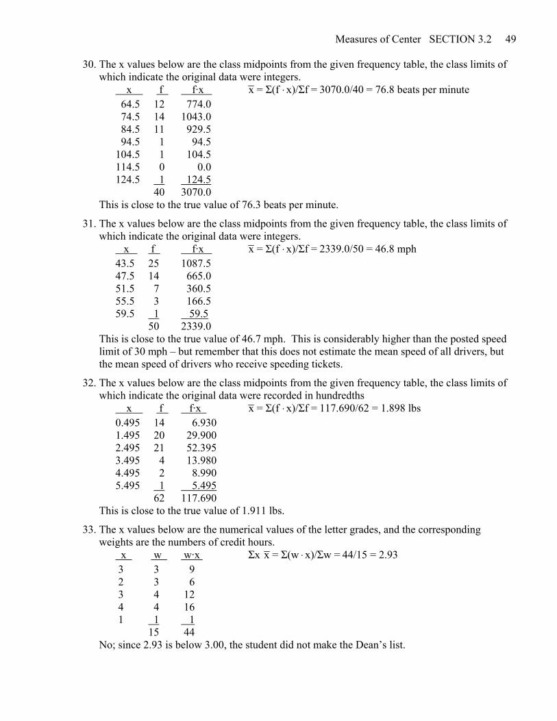
Measures of Center SECTION 3.2 49 30. The x values below are the class midpoints from the given frequency table, the class limits of which indicate the original data were integers. x f f·x . x = Σ(f x)/Σf =⋅ 3070.0/40 = 76.8 beats per minute 64.5 12 774.0 74.5 14 1043.0 84.5 11 929.5 94.5 1 94.5 104.5 1 104.5 114.5 0 0.0 124.5 1 124.5 40 3070.0 This is close to the true value of 76.3 beats per minute.

31. The x values below are the class midpoints from the given frequency table, the class limits of which indicate the original data were integers. x f f·x . x = Σ(f x)/Σf =⋅ 2339.0/50 = 46.8 mph 43.5 25 1087.5 47.5 14 665.0 51.5 7 360.5 55.5 3 166.5 59.5 1 59.5 50 2339.0 This is close to the true value of 46.7 mph. This is considerably higher than the posted speed limit of 30 mph – but remember that this does not estimate the mean speed of all drivers, but the mean speed of drivers who receive speeding tickets.

32. The x values below are the class midpoints from the given frequency table, the class limits of which indicate the original data were recorded in hundredths x f f·x . x = Σ(f x)/Σf =⋅ 117.690/62 = 1.898 lbs 0.495 14 6.930 1.495 20 29.900 2.495 21 52.395 3.495 4 13.980 4.495 2 8.990 5.495 1 5.495 62 117.690 This is close to the true value of 1.911 lbs.

33. The x values below are the numerical values of the letter grades, and the corresponding weights are the numbers of credit hours. x w w·x . xΣ x = Σ(w x)/Σw =⋅ 44/15 = 2.93 3 3 9 2 3 6 3 4 12 4 4 16 1 1 1 15 44 No; since 2.93 is below 3.00, the student did not make the Dean’s list.

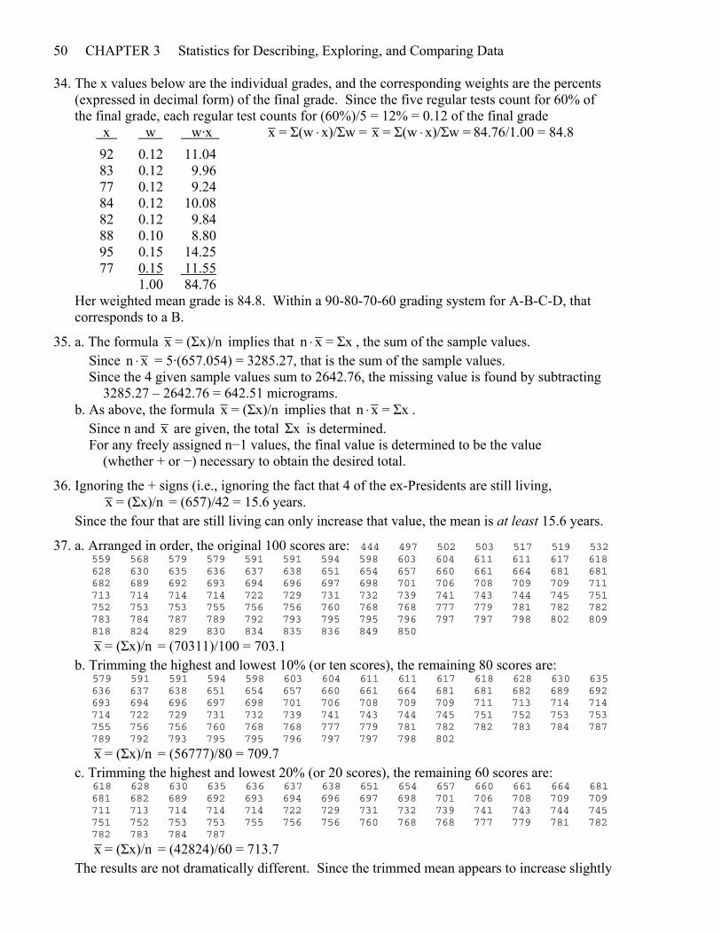
50 CHAPTER 3 Statistics for Describing, Exploring, and Comparing Data 34. The x values below are the individual grades, and the corresponding weights are the percents (expressed in decimal form) of the final grade. Since the five regular tests count for 60% of the final grade, each regular test counts for (60%)/5 = 12% = 0.12 of the final grade x w w·x . x = Σ(w x)/Σw =⋅ x = Σ(w x)/Σw =⋅ 84.76/1.00 = 84.8 92 0.12 11.04 83 0.12 9.96 77 0.12 9.24 84 0.12 10.08 82 0.12 9.84 88 0.10 8.80 95 0.15 14.25 77 0.15 11.55 1.00 84.76 Her weighted mean grade is 84.8. Within a 90-80-70-60 grading system for A-B-C-D, that corresponds to a B.

35. a. The formula x = (Σx)/n implies that n x = Σx⋅ , the sum of the sample values. Since n x⋅ = 5·(657.054) = 3285.27, that is the sum of the sample values. Since the 4 given sample values sum to 2642.76, the missing value is found by subtracting 3285.27 – 2642.76 = 642.51 micrograms. b. As above, the formula x = (Σx)/n implies that n x = Σx⋅ . Since n and x are given, the total xΣ is determined. For any freely assigned n−1 values, the final value is determined to be the value (whether + or −) necessary to obtain the desired total.

36. Ignoring the + signs (i.e., ignoring the fact that 4 of the ex-Presidents are still living, x = (Σx)/n = (657)/42 = 15.6 years. Since the four that are still living can only increase that value, the mean is at least 15.6 years.

37. a. Arranged in order, the original 100 scores are: 444 497 502 503 517 519 532 559 568 579 579 591 591 594 598 603 604 611 611 617 618 628 630 635 636 637 638 651 654 657 660 661 664 681 681 682 689 692 693 694 696 697 698 701 706 708 709 709 711 713 714 714 714 722 729 731 732 739 741 743 744 745 751 752 753 753 755 756 756 760 768 768 777 779 781 782 782 783 784 787 789 792 793 795 795 796 797 797 798 802 809 818 824 829 830 834 835 836 849 850

x = (Σx)/n = (70311)/100 = 703.1 b. Trimming the highest and lowest 10% (or ten scores), the remaining 80 scores are: 579 591 591 594 598 603 604 611 611 617 618 628 630 635 636 637 638 651 654 657 660 661 664 681 681 682 689 692 693 694 696 697 698 701 706 708 709 709 711 713 714 714 714 722 729 731 732 739 741 743 744 745 751 752 753 753 755 756 756 760 768 768 777 779 781 782 782 783 784 787 789 792 793 795 795 796 797 797 798 802

x = (Σx)/n = (56777)/80 = 709.7 c. Trimming the highest and lowest 20% (or 20 scores), the remaining 60 scores are: 618 628 630 635 636 637 638 651 654 657 660 661 664 681 681 682 689 692 693 694 696 697 698 701 706 708 709 709 711 713 714 714 714 722 729 731 732 739 741 743 744 745 751 752 753 753 755 756 756 760 768 768 777 779 781 782 782 783 784 787

x = (Σx)/n = (42824)/60 = 713.7 The results are not dramatically different. Since the trimmed mean appears to increase slightly

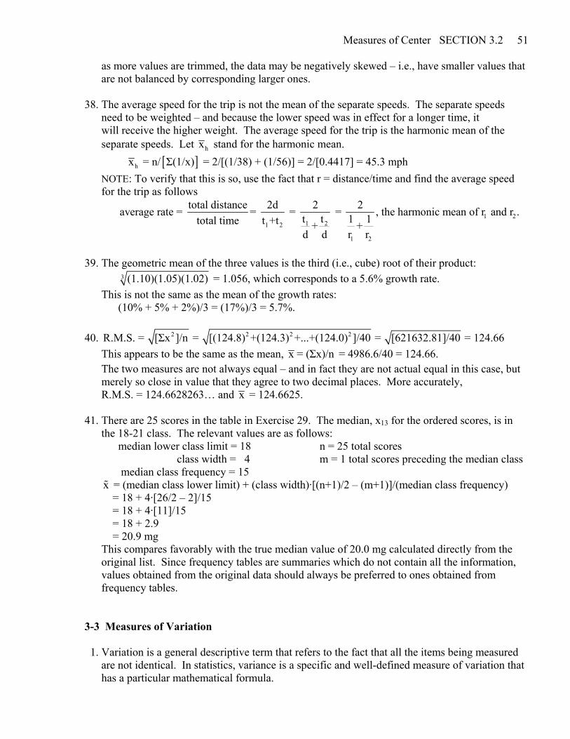
Measures of Center SECTION 3.2 51 as more values are trimmed, the data may be negatively skewed – i.e., have smaller values that are not balanced by corresponding larger ones. 38. The average speed for the trip is not the mean of the separate speeds. The separate speeds need to be weighted – and because the lower speed was in effect for a longer time, it will receive the higher weight. The average speed for the trip is the harmonic mean of the separate speeds. Let hx stand for the harmonic mean. [ ]hx = n/ Σ(1/x) = 2/[(1/38) + (1/56)] = 2/[0.4417] = 45.3 mph NOTE: To verify that this is so, use the fact that r = distance/time and find the average speed for the trip as follows

1 21 21 2

1 2

total distance 2d 2 2average rate = = = = , the harmonic mean of r and r .t t 1 1total time t +t ++r rd d

39. The geometric mean of the three values is the third (i.e., cube) root of their product: 3 (1.10)(1.05)(1.02) = 1.056, which corresponds to a 5.6% growth rate. This is not the same as the mean of the growth rates: (10% + 5% + 2%)/3 = (17%)/3 = 5.7%. 40. 2 2 2 2R.M.S. = [Σx ]/n = [(124.8) +(124.3) +...+(124.0) ]/40 = [621632.81]/40 = 124.66 This appears to be the same as the mean, x = (Σx)/n = 4986.6/40 = 124.66. The two measures are not always equal – and in fact they are not actual equal in this case, but merely so close in value that they agree to two decimal places. More accurately, R.M.S. = 124.6628263… and x = 124.6625. 41. There are 25 scores in the table in Exercise 29. The median, x13 for the ordered scores, is in the 18-21 class. The relevant values are as follows: median lower class limit = 18 n = 25 total scores class width = 4 m = 1 total scores preceding the median class median class frequency = 15 x = (median class lower limit) + (class width)·[(n+1)/2 – (m+1)]/(median class frequency) = 18 + 4·[26/2 – 2]/15 = 18 + 4·[11]/15 = 18 + 2.9 = 20.9 mg This compares favorably with the true median value of 20.0 mg calculated directly from the original list. Since frequency tables are summaries which do not contain all the information, values obtained from the original data should always be preferred to ones obtained from frequency tables. 3-3 Measures of Variation 1. Variation is a general descriptive term that refers to the fact that all the items being measured are not identical. In statistics, variance is a specific and well-defined measure of variation that has a particular mathematical formula.

52 CHAPTER 3 Statistics for Describing, Exploring, and Comparing Data 2. While that statement may give a good approximation of the standard deviation in some cases, it contains a major inaccuracy. That statement uses only the highest and lowest values to approximate the standard deviation, while the standard deviation is actually calculated using all the data values. Since the standard deviation is an attempt to measure the “typical spread,” it would not be wise to base its value on the most extreme scores in the set.

3. The incomes of the adults selected from the general population should have more variation. Statistics teachers are a more homogeneous group – they would tend to have similar salaries that would not be likely to include the extremely high or extremely low salaries possible in the general population.

4. A value is considered unusual if it differs from the mean by more than two standard deviations. Since 181 differs from the mean by (181 – 110.8)/17.1 = 4.11 standard deviations, in this context it would be considered an unusual value.

NOTE: Although not given in the text, the symbol R will be used for the range throughout this manual. Remember that the range is the difference between the highest and the lowest scores, and not necessarily the difference between the last and first scores as they are listed. Since calculating the range involves only the subtraction of 2 original pieces of data, the manual follows the advice in this section that “In general, the range should not be rounded” and reports the range with the same accuracy found in the original data. In general, the standard deviation and the variance will be reported with one more decimal place than the original data. When finding the square root of the variance to obtain the standard deviation, use all the decimal places of the variance – and not the rounded value reported as the answer. To do this, keep the value on the calculator display or place it in the memory. Do not copy down all the decimal places and then re-enter them to find the square root – as that not only is a waste of time, but also could introduce copying and/or round-off errors.

5. preliminary values: n = 10 Σx = 533 Σx2 = 30615 R = 79 – 34 = 45 words s2 = [n(Σx2) – (Σx)2]/[n(n-1)] = [10(30615) – (533)2]/[10(9)] = 22061/90 = 245.1 words2 s = 245.1 = 15.7 words There seems to be considerable variation from page to page. For small samples with n = 10, there could be considerable variation in the sample mean and, therefore, considerable variation in the projected totals for the entire dictionary. It appears that there would be a question about the accuracy of an estimate based on this sample for the total number of words.

NOTE: The above format will be used in this manual for calculation of the variance and standard deviation. To reinforce some of the key symbols and concepts, the following detailed mathematical analysis is given for the data of the above problem. x x- x (x- x)2 x2

34 -19.3 372.49 1156 x= (Σx)/n = 533/10 = 53.3 words 36 -17.3 299.29 1296 39 -14.3 204.49 1521 by formula 3-4, s2 = Σ(x- x)2/(n-1) 43 -10.3 106.09 1849 = 2206.10/9 51 -2.3 5.29 2601 = 245.1222 words2 53 -0.3 0.09 2809 62 8.7 75.69 3844 by formula 3-5, s2 = [n(Σx2) – (Σx)2]/[n(n-1) 63 9.7 94.09 3969 = [10(30615) – (533)2]/[10(9)] 73 19.7 388.09 5329 = 22061/90 79 25.7 660.49 6241 = 245.1222 words2 533 0.0 2206.10 30615

Measures of Variation SECTION 3.3 53

NOTE: As shown in the preceding detailed mathematical analysis, formulas 3-4 and 3-5 give the same answer. The following three observations give hints for using these two formulas. • When using formula 3-4, constructing a table having the first 3 columns shown above helps to organize the calculations and makes errors less likely. In addition, verify that Σ(x- x ) = 0 [except for a possible discrepancy at the last decimal due to rounding] before proceeding – if such is not the case, an error has been made and further calculation is fruitless. • When using formula 3-5, the quantity [n(Σx2) – (Σx)2] must be non-negative (i.e., greater than or equal to zero) – if such is not the case, an error has been made and further calculation is fruitless. • In general, formula 3-5 is to be preferred over formula 3-4 because (1) it does not involve round-off error or messy calculations when the mean does not “come out even” and (2) the quantities Σx and Σx2 can be found directly (on most calculators, with one pass through the data) without having to construct a table or make a second pass through the data after finding the mean.

6. preliminary values: n = 6 Σx = 4222 Σx2 = 3342798 R = 1210 – 431 = 779 hic s2 = [n(Σx2) – (Σx)2]/[n(n-1)] = [6(3342798) – (4222)2]/[6(5)] = 2231504/30 = 74383.5 hic2 s = 74383.5 =272.7 hic Yes, there seems to be much variation – mainly due to the largest value, which appears to be substantially different from the others.

7. preliminary values: n = 5 Σx = 32061 Σx2 = 220431831 R = 9052 – 4227 = $4774 s2 = [n(Σx2) – (Σx)2]/[n(n-1)] = [5(220431831) – (32061)2]/[5(4)] = 74251434/20 = 3712571.7 dollars2 s = 3712571.7 = $1926.8 A value is considered unusual if it differs from the mean by more than two standard deviations. Since $10,000 differs from the mean by (10,000 – 6,412.2)/1926.8 = 1.86 standard deviations, in this context it would not be considered an unusual value.

8. preliminary values: n = 12 Σx = 9131 Σx2 = 6985297 R = 836 – 664 = 172 points s2 = [n(Σx2) – (Σx)2]/[n(n-1)] = [12(6985297) – (9131)2]/[12(11)] = 448403/132 = 3397.0 points2 s = 3397.0 = 58.3 points A value is considered unusual if it differs from the mean by more than two standard deviations. Since 500 points differs from the mean by (500 – 760.9)/58.3 = -4.48 standard deviations, in this context it would be considered an unusual value.

9. preliminary values: n = 10 Σx = 204 Σx2 = 5494.72 R = 38 – 8.4 = $29.6 million s2 = [n(Σx2) – (Σx)2]/[n(n-1)] = [10(5494.72) – (204)2]/[10(9)] = 13331.2/90 = 148.1 (million dollars)2 s = 148.1 = $12.2 million No. The variation among the top ten salaries reveals essentially nothing about the variation of the salaries in general. All that can be said is that the range of salaries in the general population of TV personalities must be at least $29.6 million.

54 CHAPTER 3 Statistics for Describing, Exploring, and Comparing Data 10. preliminary values: n = 25 Σx = 47 Σx2 = 109 R = 4 – 1 = 3 s2 = [n(Σx2) – (Σx)2]/[n(n-1)] = [25(109) – (47)2]/[25(24)] = 516/600 = 0.86 s = 0.86 = 0.9 Yes, measures of variation can be calculated using the usual formulas. No, the results do not make sense. Since the data is collected at the nominal level, numerical calculations are not appropriate. Re-numbering the phenotypes would not actually change the results, but it would give different numerical values to the calculated measures.

11. preliminary values: n = 15 Σx = 3260 Σx2 = 865574 R = 381 – 0 = 381 hrs s2 = [n(Σx2) – (Σx)2]/[n(n-1)] = [15(865574) – (3260)2]/[15(14)] = 23356010/210 = 11219.1 hrs2 s = 11219.1 = 105.9 hrs A value is considered unusual if it differs from the mean by more than two standard deviations. Since 0 hours differs from the mean by (0 – 217.3)/105.9 = -2.05 standard deviations, in this context it would be considered an unusual value.

12. preliminary values: n = 18 Σx = 34 Σx2 = 344 R = 11 – (-5) = 16 kg s2 = [n(Σx2) – (Σx)2]/[n(n-1)] = [18(344) – (34)2]/[18(17)] = 5036/306 = 16.5 kg2 s = 16.5 = 4.1 kg A value is considered unusual if it differs from the mean by more than two standard deviations. Since 6.8 kg differs from the mean by (6.8 – 1.89)/4.06 = 1.21 standard deviations, in this context it would not be considered an unusual value. While such a weight gain is not unusual, any support such a value offers for the legend of the “freshman 15” is offset by the other data.

13. preliminary values: n = 20 Σx = 47 Σx2 = 121 R = 4 – 1 = 3 mpg s2 = [n(Σx2) – (Σx)2]/[n(n-1)] = [20(121) – (47)2]/[20(19)] = 211/380 = 0.6 (mpg)2 s = 0.6 = 0.7 mpg A value is considered unusual if it differs from the mean by more than two standard deviations. Since 4 mpg differs from the mean by (4 – 2.35)/0.75 = 2.21 standard deviations, in this context it would be considered an unusual value.

14. preliminary values: n = 8 Σx = 3662993 Σx2 = 2643662981475 R = 1,231,421 – 150,000 = $1,081,421 s2 = [n(Σx2) – (Σx)2]/[n(n-1)] = [8(2643662981475) – (3662993)2]/[8(7)] = 7731786133751/56 = 138,067,609,530.4 (dollars)2 s = 138,067,609,530.4 = $371,574.5 If the highest salary is omitted, the standard deviation drops to $217,031.6. The change is substantial. NOTE: Use the formula again. The new Σx and Σx2 may be found by subtracting from the above totals, and the n is reduced by 1.

15. preliminary values: n = 16 Σx = 4154 Σx2 = 1123116 R = 448 – 213 = 235 sec s2 = [n(Σx2) – (Σx)2]/[n(n-1)] = [16(1123116) – (4154)2]/[16(15)] = 714140/240 = 2975.6 sec2 s = 2975.6 = 54.5 sec If the highest playing time is omitted, the standard deviation drops to 22.0 sec. The change is

Measures of Variation SECTION 3.3 55 substantial. NOTE: Use the formula again. The new Σx and Σx2 may be found by subtracting from the above totals, and the n is reduced by 1.

16. preliminary values: n = 24 Σx = 259 Σx2 = 26017 R = 158 – 1 = 157 satellites s2 = [n(Σx2) – (Σx)2]/[n(n-1)] = [24(26017) – (259)2]/[24(23)] = 557327/552 = 1009.7 satellites2 s = 31.8 satellites A value is considered unusual if it differs from the mean by more than two standard deviations. Since 0 satellites differs from the mean by (0 – 10.8)/31.8 = -0.34 standard deviations, in this context it would not be considered an unusual value. NOTE: Consideration of a country with 0 satellites may not be valid in this context. Since there are many countries with 0 satellites, and since the original data included no 0’s, it appears that the data was gathered only from countries that had at least one satellite. Since countries with 0 satellites may not have been eligible for inclusion in the data, the data should not be used to make statements about such countries.

17. preliminary values: n = 20 Σx = 130 Σx2 = 1078.50 R = 15 – 4 = 11 yrs s2 = [n(Σx2) – (Σx)2]/[n(n-1)] = [20(1078.50) – (130)2]/[20(19)] = 4670/380 = 12.3 yrs2 s = 3.5 yrs A value is considered unusual if it differs from the mean by more than two standard deviations. Since 12 years differs from the mean by (12 – 6.5)/3.5 = 1.57 standard deviations, in this context it would not be considered an unusual value.

18. preliminary values: n = 8 Σx = 60.8 Σx2 = 467.24 R = 9.3 – 6.5 = 2.8 tons s2 = [n(Σx2) – (Σx)2]/[n(n-1)] = [8(467.24) – (60.8)2]/[8(7)] = 41.28/56 = 0.74 tons2 s = 0.86 tons A value is considered unusual if it differs from the mean by more than two standard deviations. Since 9.3 tons differs from the mean by (9.3 – 7.60)/0.86 = 1.98 standard deviations, in this context it would not be considered an unusual value.

19. preliminary values: n = 12 Σx = 1320 Σx2 = 236580 R = 371 – 14 = 357 bankruptcies s2 = [n(Σx2) – (Σx)2]/[n(n-1)] = [12(236580) – (1320)2]/[12(11)] = 1096560/132 = 8307.3 bankruptcies2 s = 91.1 bankruptcies A value is considered unusual if it differs from the mean by more than two standard deviations. Since 371 bankruptcies differs from the mean by (371 – 110.0)/91.1 = 2.86 standard deviations, in this context it would be considered an unusual value. None of the other given values meets that criterion.

20. preliminary values: n = 40 Σx = 5966 Σx2 = 898586 R = 188 – 114 = 74 mBq s2 = [n(Σx2) – (Σx)2]/[n(n-1)] = [40(898586) – (5966)2]/[40(39)] = 350284/1560 = 224.5 mBq2 s = 15.0 mBq A value is considered unusual if it differs from the mean by more than two standard deviations. In this context, any value less than 149.15−2(14.98) = 119.2 mBq or greater than 149.25+2(14.98) = 179.1 mBq would be considered an unusual value. Those values are: 114, 116 and 188.

56 CHAPTER 3 Statistics for Describing, Exploring, and Comparing Data

NOTE: In exercises 21 -24, CV = s/ x is found by storing the value of x and dividing the unrounded s by the unrounded stored value of x . Using the rounded values of x and s may produce slight different values as indicated. The CV is expressed as a percent.

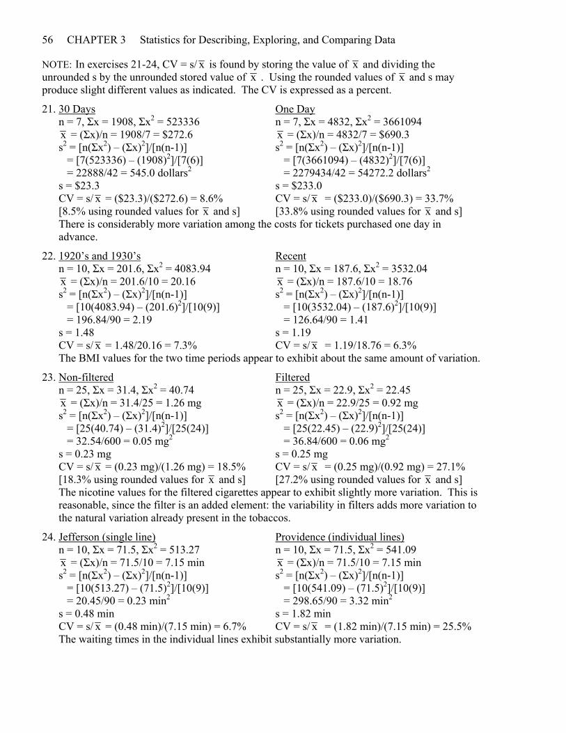
21. 30 Days One Day n = 7, Σx = 1908, Σx2 = 523336 n = 7, Σx = 4832, Σx2 = 3661094 x = (Σx)/n = 1908/7 = $272.6 x = (Σx)/n = 4832/7 = $690.3 s2 = [n(Σx2) – (Σx)2]/[n(n-1)] s2 = [n(Σx2) – (Σx)2]/[n(n-1)] = [7(523336) – (1908)2]/[7(6)] = [7(3661094) – (4832)2]/[7(6)] = 22888/42 = 545.0 dollars2 = 2279434/42 = 54272.2 dollars2 s = $23.3 s = $233.0 CV = s/ x = ($23.3)/($272.6) = 8.6% CV = s/ x = ($233.0)/($690.3) = 33.7% [8.5% using rounded values for x and s] [33.8% using rounded values for x and s] There is considerably more variation among the costs for tickets purchased one day in advance.

22. 1920’s and 1930’s Recent n = 10, Σx = 201.6, Σx2 = 4083.94 n = 10, Σx = 187.6, Σx2 = 3532.04 x = (Σx)/n = 201.6/10 = 20.16 x = (Σx)/n = 187.6/10 = 18.76 s2 = [n(Σx2) – (Σx)2]/[n(n-1)] s2 = [n(Σx2) – (Σx)2]/[n(n-1)] = [10(4083.94) – (201.6)2]/[10(9)] = [10(3532.04) – (187.6)2]/[10(9)] = 196.84/90 = 2.19 = 126.64/90 = 1.41 s = 1.48 s = 1.19 CV = s/ x = 1.48/20.16 = 7.3% CV = s/ x = 1.19/18.76 = 6.3% The BMI values for the two time periods appear to exhibit about the same amount of variation.

23. Non-filtered Filtered n = 25, Σx = 31.4, Σx2 = 40.74 n = 25, Σx = 22.9, Σx2 = 22.45 x = (Σx)/n = 31.4/25 = 1.26 mg x = (Σx)/n = 22.9/25 = 0.92 mg s2 = [n(Σx2) – (Σx)2]/[n(n-1)] s2 = [n(Σx2) – (Σx)2]/[n(n-1)] = [25(40.74) – (31.4)2]/[25(24)] = [25(22.45) – (22.9)2]/[25(24)] = 32.54/600 = 0.05 mg2 = 36.84/600 = 0.06 mg2 s = 0.23 mg s = 0.25 mg CV = s/ x = (0.23 mg)/(1.26 mg) = 18.5% CV = s/ x = (0.25 mg)/(0.92 mg) = 27.1% [18.3% using rounded values for x and s] [27.2% using rounded values for x and s] The nicotine values for the filtered cigarettes appear to exhibit slightly more variation. This is reasonable, since the filter is an added element: the variability in filters adds more variation to the natural variation already present in the tobaccos.

24. Jefferson (single line) Providence (individual lines) n = 10, Σx = 71.5, Σx2 = 513.27 n = 10, Σx = 71.5, Σx2 = 541.09 x = (Σx)/n = 71.5/10 = 7.15 min x = (Σx)/n = 71.5/10 = 7.15 min s2 = [n(Σx2) – (Σx)2]/[n(n-1)] s2 = [n(Σx2) – (Σx)2]/[n(n-1)] = [10(513.27) – (71.5)2]/[10(9)] = [10(541.09) – (71.5)2]/[10(9)] = 20.45/90 = 0.23 min2 = 298.65/90 = 3.32 min2 s = 0.48 min s = 1.82 min CV = s/ x = (0.48 min)/(7.15 min) = 6.7% CV = s/ x = (1.82 min)/(7.15 min) = 25.5% The waiting times in the individual lines exhibit substantially more variation.

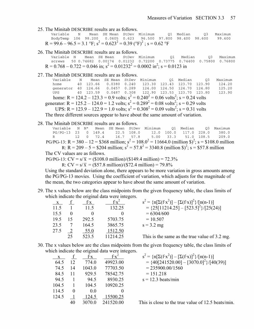
Measures of Variation SECTION 3.3 57 25. The Minitab DESCRIBE results are as follows. Variable N Mean SE Mean StDev Minimum Q1 Median Q3 Maximum BodyTemp 106 98.200 0.0605 0.623 96.500 97.800 98.400 98.600 99.600

R = 99.6 – 96.5 = 3.1 °F; s2 = 0.6232 = 0.39 (°F)2 ; s = 0.62 °F

26. The Minitab DESCRIBE results are as follows. Variable N Mean SE Mean StDev Minimum Q1 Median Q3 Maximum screws 50 0.74682 0.00174 0.01232 0.72200 0.73775 0.74400 0.75800 0.76800

R = 0.768 – 0.722 = 0.046 in; s2 = 0.012322 = 0.0002 in2; s = 0.0123 in

27. The Minitab DESCRIBE results are as follows. Variable N Mean SE Mean StDev Minimum Q1 Median Q3 Maximum home 40 123.66 0.0380 0.240 123.30 123.43 123.70 123.90 124.20 generator 40 124.66 0.0457 0.289 124.00 124.50 124.70 124.80 125.20 UPS 40 123.59 0.0487 0.308 122.90 123.53 123.70 123.80 123.90

home: R = 124.2 – 123.3 = 0.9 volts; s2 = 0.2402 = 0.06 volts2; s = 0.24 volts generator: R = 125.2 – 124.0 = 1.2 volts; s2 = 0.2892 = 0.08 volts2; s = 0.29 volts UPS: R = 123.9 – 122.9 = 1.0 volts; s2 = 0.3082 = 0.09 volts2; s = 0.31 volts The three different sources appear to have about the same amount of variation.

28. The Minitab DESCRIBE results are as follows. Variable N N* Mean SE Mean StDev Minimum Q1 Median Q3 Maximum PG/PG-13 23 0 149.4 22.5 108.0 12.0 100.0 117.0 228.0 380.0 R 12 0 72.4 16.7 57.8 5.00 33.3 51.0 108.5 209.0

PG/PG-13: R = 380 – 12 = $368 million; s2 = 108.02 = 11664.0 (million $)2; s = $108.0 million R: R = 209 – 5 = $204 million; s2 = 57.82 = 3340.8 (million $)2; s = $57.8 million The CV values are as follows. PG/PG-13: CV = s/ x = ($108.0 million)/($149.4 million) = 72.3% R: CV = s/ x = ($57.8 million)/($72.4 million) = 79.8% Using the standard deviation alone, there appears to be more variation in gross amounts among the PG/PG-13 movies. Using the coefficient of variation, which adjusts for the magnitude of the mean, the two categories appear to have about the same amount of variation.

29. The x values below are the class midpoints from the given frequency table, the class limits of which indicate the original data were integers. x f f·x f·x2 s2 = {n[Σ(f·x2)] – [Σ(f·x)]2}/[n(n-1)] 11.5 1 11.5 132.25 = {25[11214.25] – [523.5]2}/[25(24)] 15.5 0 0 0 = 6304/600 19.5 15 292.5 5703.75 = 10.507 23.5 7 164.5 3865.75 s = 3.2 mg 27.5 2 55.0 1512.50 25 523.5 11214.25 This is the same as the true value of 3.2 mg.

30. The x values below are the class midpoints from the given frequency table, the class limits of which indicate the original data were integers. x f f·x f·x2 s2 = {n[Σ(f·x2)] – [Σ(f·x)]2}/[n(n-1)] 64.5 12 774.0 49923.00 = {40[241520.00] – [3070.0]2}/[40(39)] 74.5 14 1043.0 77703.50 = 235900.00/1560 84.5 11 929.5 78542.75 = 151.218 94.5 1 94.5 8930.25 s = 12.3 beats/min 104.5 1 104.5 10920.25 114.5 0 0.0 0 124.5 1 124.5 15500.25 40 3070.0 241520.00 This is close to the true value of 12.5 beats/min.

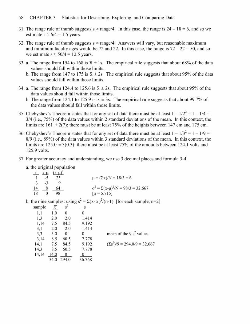
58 CHAPTER 3 Statistics for Describing, Exploring, and Comparing Data 31. The range rule of thumb suggests s ≈ range/4. In this case, the range is 24 – 18 = 6, and so we estimate s ≈ 6/4 = 1.5 years.

32. The range rule of thumb suggests s ≈ range/4. Answers will vary, but reasonable maximum and minimum faculty ages would be 72 and 22. In this case, the range is 72 – 22 = 50, and so we estimate s ≈ 50/4 = 12.5 years.

33. a. The range from 154 to 168 is x ± 1s. The empirical rule suggests that about 68% of the data values should fall within those limits. b. The range from 147 to 175 is x ± 2s. The empirical rule suggests that about 95% of the data values should fall within those limits.

34. a. The range from 124.4 to 125.6 is x ± 2s. The empirical rule suggests that about 95% of the data values should fall within those limits. b. The range from 124.1 to 125.9 is x ± 3s. The empirical rule suggests that about 99.7% of the data values should fall within those limits.

35. Chebyshev’s Theorem states that for any set of data there must be at least 1 – 1/22 = 1 – 1/4 = 3/4 (i.e., 75%) of the data values within 2 standard deviations of the mean. In this context, the limits are 161 ± 2(7): there must be at least 75% of the heights between 147 cm and 175 cm.

36. Chebyshev’s Theorem states that for any set of data there must be at least 1 – 1/32 = 1 – 1/9 = 8/9 (i.e., 89%) of the data values within 3 standard deviations of the mean. In this context, the limits are 125.0 ± 3(0.3): there must be at least 75% of the amounts between 124.1 volts and 125.9 volts.

37. For greater accuracy and understanding, we use 3 decimal places and formula 3-4.

a. the original population x x-μ (x-μ)2 1 -5 25 μ = (Σx)/N = 18/3 = 6

3 -3 9 14 8 64 σ2 = Σ(x-μ)2/N = 98/3 = 32.667

18 0 98 [σ = 5.715]

b. the nine samples: using s2 = Σ(x- x)2/(n-1) [for each sample, n=2] sample X s2 s 1,1 1.0 0 0 1,3 2.0 2.0 1.414 1,14 7.5 84.5 9.192 3,1 2.0 2.0 1.414 3,3 3.0 0 0 mean of the 9 s2 values 3,14 8.5 60.5 7.778 14,1 7.5 84.5 9.192 (Σs2)/9 = 294.0/9 = 32.667 14,3 8.5 60.5 7.778 14,14 14.0 0 0 . 54.0 294.0 36.768

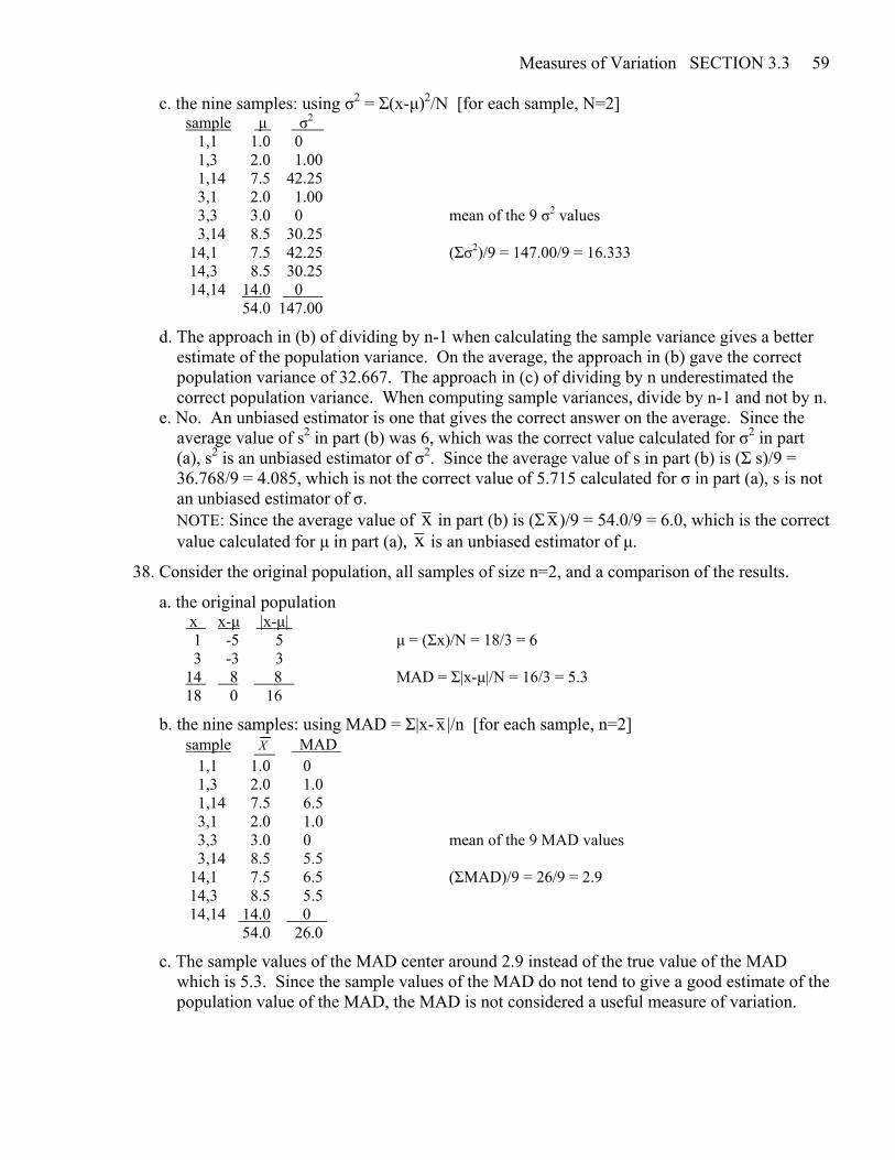
Measures of Variation SECTION 3.3 59 c. the nine samples: using σ2 = Σ(x-μ)2/N [for each sample, N=2] sample μ σ2 . 1,1 1.0 0 1,3 2.0 1.00 1,14 7.5 42.25 3,1 2.0 1.00 3,3 3.0 0 mean of the 9 σ2 values 3,14 8.5 30.25 14,1 7.5 42.25 (Σσ2)/9 = 147.00/9 = 16.333 14,3 8.5 30.25 14,14 14.0 0 . 54.0 147.00

d. The approach in (b) of dividing by n-1 when calculating the sample variance gives a better estimate of the population variance. On the average, the approach in (b) gave the correct population variance of 32.667. The approach in (c) of dividing by n underestimated the correct population variance. When computing sample variances, divide by n-1 and not by n. e. No. An unbiased estimator is one that gives the correct answer on the average. Since the average value of s2 in part (b) was 6, which was the correct value calculated for σ2 in part (a), s2 is an unbiased estimator of σ2. Since the average value of s in part (b) is (Σ s)/9 = 36.768/9 = 4.085, which is not the correct value of 5.715 calculated for σ in part (a), s is not an unbiased estimator of σ. NOTE: Since the average value of x in part (b) is (Σx)/9 = 54.0/9 = 6.0, which is the correct value calculated for μ in part (a), x is an unbiased estimator of μ.

38. Consider the original population, all samples of size n=2, and a comparison of the results.

a. the original population x x-μ |x-μ| 1 -5 5 μ = (Σx)/N = 18/3 = 6

3 -3 3 14 8 8 MAD = Σ|x-μ|/N = 16/3 = 5.3

18 0 16

b. the nine samples: using MAD = Σ|x- x |/n [for each sample, n=2] sample X MAD 1,1 1.0 0 1,3 2.0 1.0 1,14 7.5 6.5 3,1 2.0 1.0 3,3 3.0 0 mean of the 9 MAD values 3,14 8.5 5.5 14,1 7.5 6.5 (ΣMAD)/9 = 26/9 = 2.9 14,3 8.5 5.5 14,14 14.0 0 54.0 26.0

c. The sample values of the MAD center around 2.9 instead of the true value of the MAD which is 5.3. Since the sample values of the MAD do not tend to give a good estimate of the population value of the MAD, the MAD is not considered a useful measure of variation.

60 CHAPTER 3 Statistics for Describing, Exploring, and Comparing Data 3-4 Measures of Relative Standing and Boxplots 1. For a z score of -0.61, the negative sign indicates that her age is below the mean and the numerical portion indicates that her age is 0.61 standard deviations away from the mean.

2. The z score will have no units. Since the numerator x− x is measured in centimeters and the denominator s is measured in centimeters, the units “cancel out” and the quotient z = (x − x )/s is unit-free.

3. The values shown in the boxplot constitute the 5-number summary as follows. 0 hours = the minimum value, the length of the shortest flight 166 hours = the first quartile Q1, the length below which the shortest 25% of the flights occur 215 hours = the second quartile Q2, the median length of the flights 269 hours = the third quartile Q3, the length above which the longest 25% of the flights occur 423 hours = the maximum value, the length of the longest flight

4. The bottom boxplot represents the weights of the women, because the weights it depicts are generally lower. The bottom boxplot depicts weights with more variation, because the boxes from Q1 to Q3 are about the same length but the overall line from the minimum to the maximum is longer.

5. a. |x – x | = |61 – 35.8| = |25.2| = 25.2 years b. 25.2/11.3 = 2.23 c. z = (x− x )/s = (61−35.8)/11.3 = 2.23 d. Since 2.23 > 2.00, Helen Mirren’s age is considered unusual in this context.

6. a. |x – x | = |38 – 43.8| = |-5.8| = 5.8 years b. 5.8/8.9 = 0.65 c. z = (x − x )/s = (38 − 43.8)/8.9 = -0.65 d. Since -2.00 < -0.65 < 2.00, P.S. Hoffman’s age is not considered unusual in this context.

7. a. |x – x | = |110 – 245.0| = |-135.0| = 135.0 seconds b. 135.0/36.4 = 3.71 c. z = (x − x )/s = (110 − 245.0)/36.4 = -3.71 d. Since -3.71 < -2.00, a duration time of 110 seconds is considered unusual in this context.

8. a. |x – x | = |92.95 – 69.6| = |23.35| = 23.35 inches b. 23.35/2.8 = 8.34 c. z = (x − x )/s = (92.95 − 69.6)/2.8 = 8.34 d. Since 8.34 > 2.00, Bao Xishun’s height is considered unusual in this context.

9. a. z = (x − x )/s = (101.00 − 98.20)/0.62 = 4.52; unusual, since 4.52 > 2.00 b. z = (x − x )/s = (96.90 − 98.20)/0.62 = -2.10; unusual, since -2.10 < -2.00 c. z = (x − x )/s = (96.98 − 98.20)/0.62 = -1.97; usual, since -2.00 < -1.97 < 2.00

10. minimum: z = (x− x )/s = (58−63.6)/2.5 = -2.24; unusual, since -2.24 < -2.00 maximum: z = (x− x )/s = (80−63.6)/2.5 = 6.56; unusual, since 6.56 > 2.00

11. z = (x – x)/s = (308 – 268)/15 = 40/15 = 2.67 Yes, since 2.67 > 2.00, a pregnancy of 308 days is considered unusual. “Unusual” is just what the word implies – out of the ordinary. Other exercises in this section note that there are unusual ages and heights, and so there can be unusual pregnancies.

12. z = (x – x)/s = (16.60 – 7.14)/2.51 = 9.46/2.51 = 3.77 Yes, since 3.77 > 2.00, a white blood cell count of 16.60 is considered unusual.

Measures of Relative Standing and Boxplots SECTION 3.4 61 13. SAT: z = (x – x)/s = (1840 – 1518)/325 = 322/325 = 0.99 ACT: z = (x – x)/s = (26.0 – 21.1)/4.8 = 4.9/4.8 = 1.02 Since 1.02 > 0.99, the ACT score of 26.0 is the relatively better score.

14. SAT: z = (x – x)/s = (1190 – 1518)/325 = -328/325 = -1.01 ACT: z = (x – x)/s = (16.0 – 21.1)/4.8 = -5.1/4.8 = -1.06 Since -1.01 > -1.06, the SAT score of 1190 is the relatively better score.

For exercises 15-27, refer to the list of ordered scores at the right. The units are total points.

15. Let b = # of scores below x; n = total number of scores In general, the percentile of score x is (b/n)·100. The percentile score of 47 is (9/24)·100 = 38.

16. Let b = # of scores below x; n = total number of scores In general, the percentile of score x is (b/n)·100. The percentile score of 65 is (20/24)·100 = 83.

17. Let b = # of scores below x; n = total number of scores In general, the percentile of score x is (b/n)·100. The percentile score of 54 is (12/24)·100 = 50.

18. Let b = # of scores below x; n = total number of scores In general, the percentile of score x is (b/n)·100. The percentile score of 41 is (5/24)·100 = 21.

19. To find P20, L = (20/100)·24 = 4.8, rounded up to 5. Since the 5th score is 39, P20 = 39.

20. To find Q1 = P25, L = (25/100)·24 = 6, a whole number. The mean of the 6th and 7th scores, Q1 = (41+43)/2 = 42.

21. To find Q3 = P75, L = (75/100)·24 = 18, a whole number. The mean of the 18th and 19th scores, Q3 (59+61)/2 = 60.

22. To find P80, L = (80/100)·24 = 19.2, rounded up to 20. Since the 20th score is 61, P80 = 61.

23. To find P50, L = (50/100)·24 = 12, a whole number. The mean of the 12th and 13th scores, P50 = (53+54)/2 = 53.5.

24. To find P75, L = (75/100)·24 = 18, a whole number. The mean of the 18th and 19th scores, P75 = (59+61)/2 = 60.

25. To find P25, L = (25/100)·24 = 6, a whole number. The mean of the 6th and 7th scores, P25 = (41+43)/2 = 42.

26. To find P95, L = (95/100)·24 = 22.8, rounded up to 23. Since the 23rd score is 69, P95 = 69.

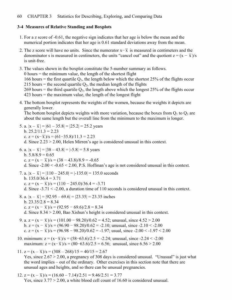
27. Arrange the 24 values in order. The 5-number summary and boxplot are given below. All measurements are in total points. min = x1 = 36 Q1 = (x6+x7)/2 = (41+43)/2 = 42 median = (x12+x13)/2 = (53+54)/2 = 53.5 Q3 = (x18+x19)/2 = (59+61)/2 = 60 max = x24 = 75

# points 1 36 2 37 3 37 4 39 5 39 6 41 7 43 8 44 9 44 10 47 11 50 12 53 13 54 14 55 15 56 16 56 17 57 18 59 19 61 20 61 21 65 22 69 23 69 24 75

62 CHAPTER 3 Statistics for Describing, Exploring, and Comparing Data

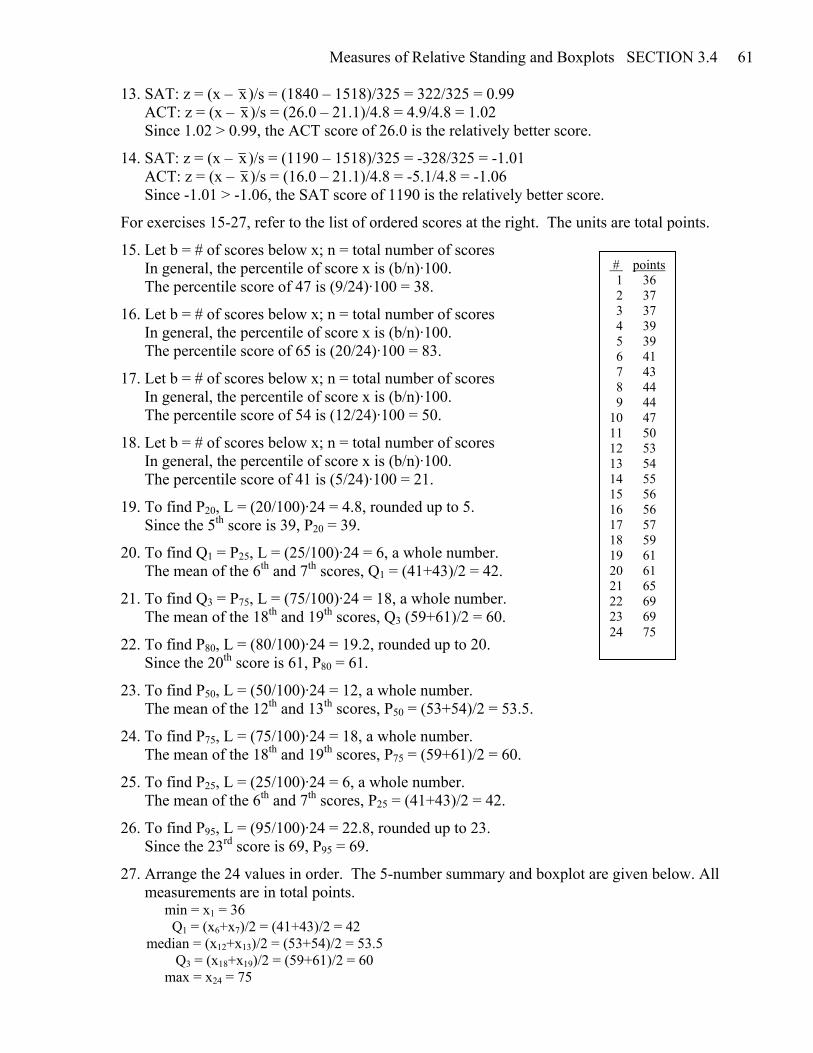
28. Arrange the 10 values in order. The 5-number summary and boxplot are given below. All measurements are in words per page. min = x1 = 34 Q1 = x3= 39 median = (x5+x6)/2 = (51+53)/2 = 52 Q3 = x8 = 63 max = x20 = 79

29. Arrange the 12 values in order. The 5-number summary and boxplot are given below. All measurements are in FICO rating units. min = x1 = 664 Q1 = (x3+x4)/2 = (698+714)/2 = 706 median = (x6+x7)/2 = (753+779)/2 = 766 Q3 = (x9+x10)/2 = (802+818)/2 = 810 max = x12 = 836

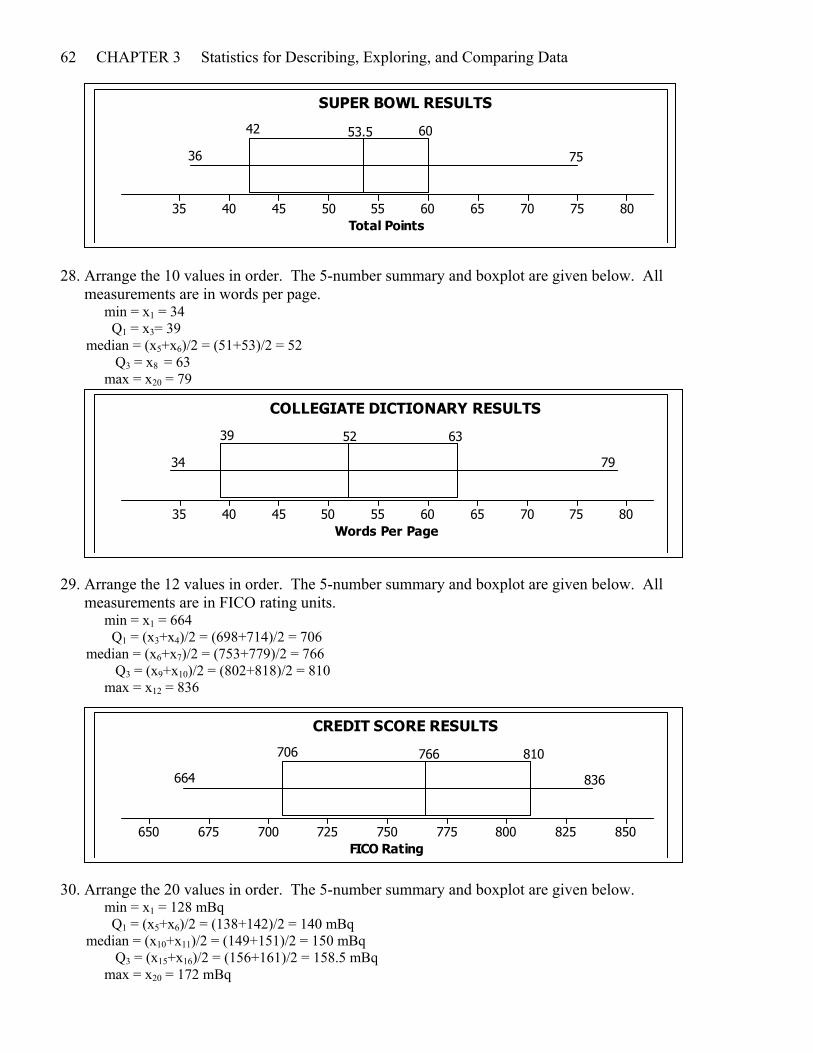
30. Arrange the 20 values in order. The 5-number summary and boxplot are given below. min = x1 = 128 mBq Q1 = (x5+x6)/2 = (138+142)/2 = 140 mBq median = (x10+x11)/2 = (149+151)/2 = 150 mBq Q3 = (x15+x16)/2 = (156+161)/2 = 158.5 mBq max = x20 = 172 mBq

Total Points80757065605550454035

SUPER BOWL RESULTS

36

42 53.5 60

75

Words Per Page80757065605550454035

COLLEGIATE DICTIONARY RESULTS

34

39 52 63

79

FICO Rating850825800775750725700675650

CREDIT SCORE RESULTS

664

706 766 810

836

Measures of Relative Standing and Boxplots SECTION 3.4 63

31. Arrange the 36 values in order. The 5-number summaries and boxplots are given below. Regular Coke min = x1 = 0.7901 lbs Q1 = (x9+x10)/2 = (0.8143+0.8150)/2 = 0.81465 lbs median = (x18+x19)/2 = (0.8170+0.8172)/2 = 0.8171 lbs Q3 = (x27+x28)/2 = (0.8207+0.8211)/2 = 0.8209 lbs max = x36 = 0.8295 lbs Diet Coke min = x1 = 0.7758 lbs Q1 = (x9+x10)/2 = (0.7822+0.7822)/2 = 0.7822 lbs median = (x18+x19)/2 = (0.7852+0.7852)/2 = 0.7852 lbs Q3 = (x27+x28)/2 = (0.7879+0.7879)/2 = 0.7879 lbs max = x36 = 0.7923 lbs

The weights of the diet Coke appear to be substantially less than those of the regular Coke.

32. Arrange the 36 values in order. The 5-number summaries and boxplots are given below. Regular Coke min = x1 = 0.7901 lbs Q1 = (x9+x10)/2 = (0.8143+0.8150)/2 = 0.81465 lbs median = (x18+x19)/2 = (0.8170+0.8172)/2 = 0.8171 lbs Q3 = (x27+x28)/2 = (0.8207+0.8211)/2 = 0.8209 lbs max = x36 = 0.8295 lbs

Strontium-90 (mBq)170165160155150145140135130

BABY TEETH RESULTS

128

140 150 158.5

172

weight (lbs)0.8280.8220.8160.8100.8040.7980.7920.7860.780

REGULAR COKE

0.7901

0.81465 0.8171 0.8209

0.8295

weight (lbs)0.8280.8220.8160.8100.8040.7980.7920.7860.780

DIET COKE

0.7758

0.7822 0.7852 0.7879

0.7923

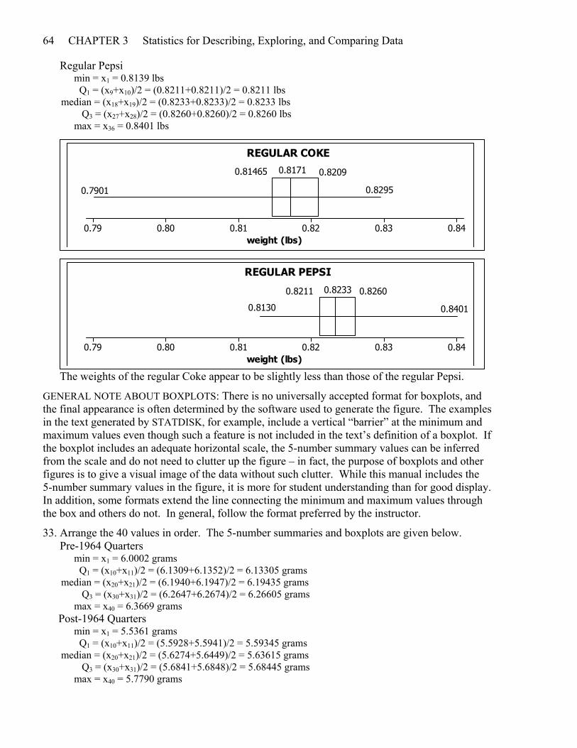
64 CHAPTER 3 Statistics for Describing, Exploring, and Comparing Data Regular Pepsi min = x1 = 0.8139 lbs Q1 = (x9+x10)/2 = (0.8211+0.8211)/2 = 0.8211 lbs median = (x18+x19)/2 = (0.8233+0.8233)/2 = 0.8233 lbs Q3 = (x27+x28)/2 = (0.8260+0.8260)/2 = 0.8260 lbs max = x36 = 0.8401 lbs

The weights of the regular Coke appear to be slightly less than those of the regular Pepsi.

GENERAL NOTE ABOUT BOXPLOTS: There is no universally accepted format for boxplots, and the final appearance is often determined by the software used to generate the figure. The examples in the text generated by STATDISK, for example, include a vertical “barrier” at the minimum and maximum values even though such a feature is not included in the text’s definition of a boxplot. If the boxplot includes an adequate horizontal scale, the 5-number summary values can be inferred from the scale and do not need to clutter up the figure – in fact, the purpose of boxplots and other figures is to give a visual image of the data without such clutter. While this manual includes the 5-number summary values in the figure, it is more for student understanding than for good display. In addition, some formats extend the line connecting the minimum and maximum values through the box and others do not. In general, follow the format preferred by the instructor.

33. Arrange the 40 values in order. The 5-number summaries and boxplots are given below. Pre-1964 Quarters min = x1 = 6.0002 grams Q1 = (x10+x11)/2 = (6.1309+6.1352)/2 = 6.13305 grams median = (x20+x21)/2 = (6.1940+6.1947)/2 = 6.19435 grams Q3 = (x30+x31)/2 = (6.2647+6.2674)/2 = 6.26605 grams max = x40 = 6.3669 grams Post-1964 Quarters min = x1 = 5.5361 grams Q1 = (x10+x11)/2 = (5.5928+5.5941)/2 = 5.59345 grams median = (x20+x21)/2 = (5.6274+5.6449)/2 = 5.63615 grams Q3 = (x30+x31)/2 = (5.6841+5.6848)/2 = 5.68445 grams max = x40 = 5.7790 grams

weight (lbs)0.840.830.820.810.800.79

REGULAR COKE

0.7901

0.81465 0.8171 0.8209

0.8295

weight (lbs)0.840.830.820.810.800.79

REGULAR PEPSI

0.8130

0.8211 0.8233 0.8260

0.8401

Measures of Relative Standing and Boxplots SECTION 3.4 65

The weights of the pre-1964 quarters are substantially greater than the weights of the post-1964 quarters.

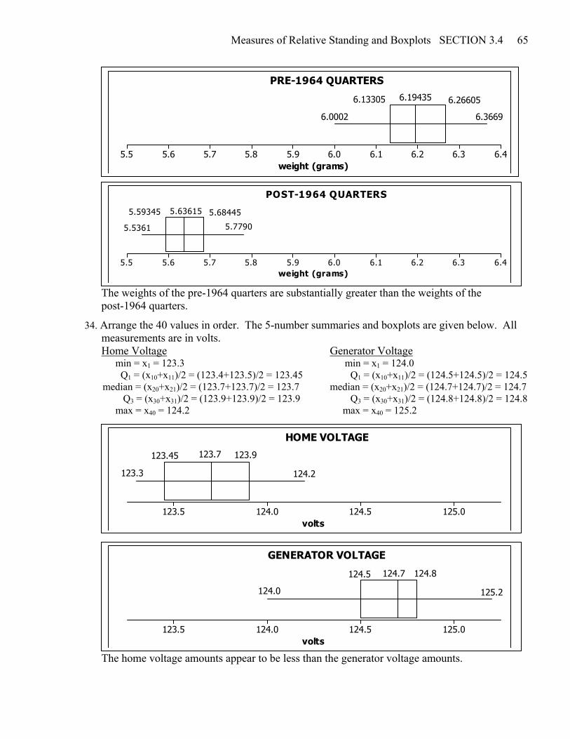
34. Arrange the 40 values in order. The 5-number summaries and boxplots are given below. All measurements are in volts. Home Voltage Generator Voltage min = x1 = 123.3 min = x1 = 124.0 Q1 = (x10+x11)/2 = (123.4+123.5)/2 = 123.45 Q1 = (x10+x11)/2 = (124.5+124.5)/2 = 124.5 median = (x20+x21)/2 = (123.7+123.7)/2 = 123.7 median = (x20+x21)/2 = (124.7+124.7)/2 = 124.7 Q3 = (x30+x31)/2 = (123.9+123.9)/2 = 123.9 Q3 = (x30+x31)/2 = (124.8+124.8)/2 = 124.8 max = x40 = 124.2 max = x40 = 125.2

The home voltage amounts appear to be less than the generator voltage amounts.

weight (grams)6.46.36.26.16.05.95.85.75.65.5

PRE-1964 QUARTERS

6.0002

6.13305 6.19435 6.26605

6.3669

weight (grams)6.46.36.26.16.05.95.85.75.65.5

POST-1964 QUARTERS

5.5361

5.59345 5.63615 5.68445

5.7790

volts125.0124.5124.0123.5

HOME VOLTAGE

123.3

123.45 123.7 123.9

124.2

volts125.0124.5124.0123.5

GENERATOR VOLTAGE

124.0

124.5 124.7 124.8

125.2

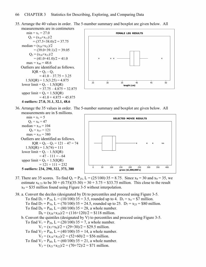
66 CHAPTER 3 Statistics for Describing, Exploring, and Comparing Data 35. Arrange the 40 values in order. The 5-number summary and boxplot are given below. All measurements are in centimeters min = x1 = 27.0 Q1 = (x10+x11)/2 = (37.5+38.0)/2 = 37.75 median = (x20+x21)/2 = (39.0+39.1)/2 = 39.05 Q3 = (x30+x31)/2 = (41.0+41.0)/2 = 41.0 max = x40 = 48.6 Outliers are identified as follows. IQR = Q3 – Q1 = 41.0 – 37.75 = 3.25 1.5(IQR) = 1.5(3.25) = 4.875 lower limit = Q1 – 1.5(IQR) = 37.75 – 4.875 = 32.875 upper limit = Q3 + 1.5(IQR) = 41.0 + 4.875 = 45.875 4 outliers: 27.0, 31.1, 32.1, 48.6

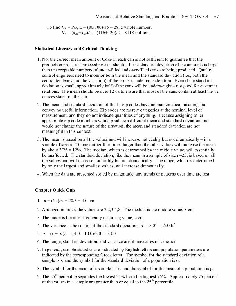
36. Arrange the 35 values in order. The 5-number summary and boxplot are given below. All measurements are in $ millions. min = x1 = 5 Q1 = x9 = 47 median = x18 = 104 Q3 = x27 = 121 max = x35 = 380 Outliers are identified as follows. IQR = Q3 – Q1 = 121 – 47 = 74 1.5(IQR) = 1.5(74) = 111 lower limit = Q1 – 1.5(IQR) = 47 – 111 = - 64 upper limit = Q3 + 1.5(IQR) = 121 + 111 = 232 5 outliers: 234, 290, 322, 373, 380 37. There are 35 scores. To find Q1 = P25, L = (25/100)·35 = 8.75. Since x8 = 30 and x9 = 35, we estimate x8.75 to be 30 + (0.75)(35-30) = 30 + 3.75 = $33.75 million. This close to the result x9 = $35 million found using Figure 3-5 without interpolation.

38. a. Convert the deciles (designated by D) to percentiles and proceed using Figure 3-5. To find D1 = P10, L = (10/100)·35 = 3.5, rounded up to 4. D1 = x4 = $7 million. To find D7 = P70, L = (70/100)·35 = 24.5, rounded up to 25. D7 = x25 = $80 million. To find D8 = P80, L = (80/100)·35 = 28, a whole number. D8 = (x28+x29)/2 = (116+120)/2 = $118 million. b. Convert the quintiles (designated by V) to percentiles and proceed using Figure 3-5. To find V1 = P20, L = (20/100)·35 = 7, a whole number. V1 = (x7+x8)/2 = (29+30)/2 = $29.5 million. To find V2 = P40, L = (40/100)·35 = 14, a whole number. V2 = (x14+x15)/2 = (52+60)/2 = $56 million. To find V3 = P60, L = (60/100)·35 = 21, a whole number. V3 = (x21+x22)/2 = (70+72)/2 = $71 million.

length (cm)504540353025

FEMALE LEG RESULTS

gross ($1,000,000's)400350300250200150100500

SELECTED MOVIE RESULTS

Measures of Relative Standing and Boxplots SECTION 3.4 67 To find V4 = P80, L = (80/100)·35 = 28, a whole number. V4 = (x28+x29)/2 = (116+120)/2 = $118 million. Statistical Literacy and Critical Thinking 1. No, the correct mean amount of Coke in each can is not sufficient to guarantee that the production process is proceeding as it should. If the standard deviation of the amounts is large, then unacceptable numbers of under-filled and over-filled cans are being produced. Quality control engineers need to monitor both the mean and the standard deviation (i.e., both the central tendency and the variation) of the process under consideration. Even if the standard deviation is small, approximately half of the cans will be underweight – not good for customer relations. The mean should be over 12 oz to ensure that most of the cans contain at least the 12 ounces stated on the can.

2. The mean and standard deviation of the 11 zip codes have no mathematical meaning and convey no useful information. Zip codes are merely categories at the nominal level of measurement, and they do not indicate quantities of anything. Because assigning other appropriate zip code numbers would produce a different mean and standard deviation, but would not change the nature of the situation, the mean and standard deviation are not meaningful in this context.

3. The mean is based on all the values and will increase noticeably but not dramatically – in a sample of size n=25, one outlier four times larger than the other values will increase the mean by about 3/25 = 12%. The median, which is determined by the middle value, will essentially be unaffected. The standard deviation, like the mean in a sample of size n=25, is based on all the values and will increase noticeably but not dramatically. The range, which is determined by only the largest and smallest values, will increase dramatically.

4. When the data are presented sorted by magnitude, any trends or patterns over time are lost. Chapter Quick Quiz 1. x = (Σx)/n = 20/5 = 4.0 cm

2. Arranged in order, the values are 2,2,3,5,8. The median is the middle value, 3 cm.

3. The mode is the most frequently occurring value, 2 cm.

4. The variance is the square of the standard deviation. s2 = 5.02 = 25.0 ft2

5. z = (x − x )/s = (4.0 – 10.0)/2.0 = -3.00

6. The range, standard deviation, and variance are all measures of variation.

7. In general, sample statistics are indicated by English letters and population parameters are indicated by the corresponding Greek letter. The symbol for the standard deviation of a sample is s, and the symbol for the standard deviation of a population is σ.

8. The symbol for the mean of a sample is x , and the symbol for the mean of a population is μ.

9. The 25th percentile separates the lowest 25% from the highest 75%. Approximately 75 percent of the values in a sample are greater than or equal to the 25th percentile.

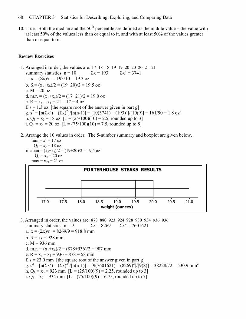
68 CHAPTER 3 Statistics for Describing, Exploring, and Comparing Data 10. True. Both the median and the 50th percentile are defined as the middle value – the value with at least 50% of the values less than or equal to it, and with at least 50% of the values greater than or equal to it. Review Exercises 1. Arranged in order, the values are: 17 18 18 19 19 20 20 20 21 21 summary statistics: n = 10 Σx = 193 Σx2 = 3741 a. x = (Σx)/n = 193/10 = 19.3 oz b. x = (x5+x6)/2 = (19+20)/2 = 19.5 oz c. M = 20 oz d. m.r. = (x1+xn)/2 = (17+21)/2 = 19.0 oz e. R = xn – x1 = 21 – 17 = 4 oz f. s = 1.3 oz [the square root of the answer given in part g] g. s2 = [n(Σx2) – (Σx)2]/[n(n-1)] = [10(3741) – (193)2]/[10(9)] = 161/90 = 1.8 oz2 h. Q1 = x3 = 18 oz [L = (25/100)(10) = 2.5, rounded up to 3] i. Q3 = x8 = 20 oz [L = (75/100)(10) = 7.5, rounded up to 8] 2. Arrange the 10 values in order. The 5-number summary and boxplot are given below. min = x1 = 17 oz Q1 = x3 = 18 oz median = (x5+x6)/2 = (19+20)/2 = 19.5 oz Q3 = x8 = 20 oz max = x10 = 21 oz

3. Arranged in order, the values are: 878 880 923 924 928 930 934 936 936 summary statistics: n = 9 Σx = 8269 Σx2 = 7601621 a. x = (Σx)/n = 8269/9 = 918.8 mm b. x = x5 = 928 mm c. M = 936 mm d. m.r. = (x1+xn)/2 = (878+936)/2 = 907 mm e. R = xn – x1 = 936 – 878 = 58 mm f. s = 23.0 mm [the square root of the answer given in part g] g. s2 = [n(Σx2) – (Σx)2]/[n(n-1)] = [9(7601621) – (8269)2]/[9(8)] = 38228/72 = 530.9 mm2 h. Q1 = x3 = 923 mm [L = (25/100)(9) = 2.25, rounded up to 3] i. Q3 = x7 = 934 mm [L = (75/100)(9) = 6.75, rounded up to 7]

weight (ounces)21.020.520.019.519.018.518.017.517.0

PORTERHOUSE STEAKS RESULTS

Review Exercises 69 4. z = (x – x )/s = (878 – 918.8)/23.0 = -1.77 No. Since -2 < -1.77 < 2, the sitting height of 878 mm is not unususal.

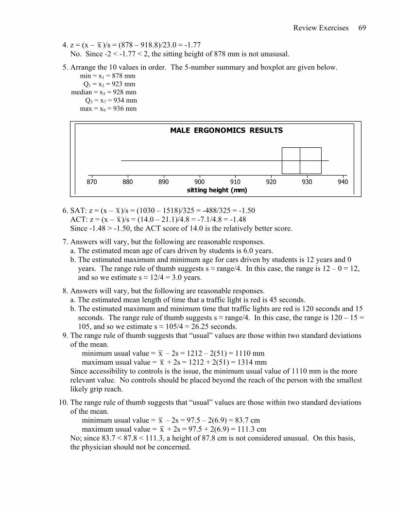
5. Arrange the 10 values in order. The 5-number summary and boxplot are given below. min = x1 = 878 mm Q1 = x3 = 923 mm median = x5 = 928 mm Q3 = x7 = 934 mm max = x9 = 936 mm

6. SAT: z = (x – x)/s = (1030 – 1518)/325 = -488/325 = -1.50 ACT: z = (x – x)/s = (14.0 – 21.1)/4.8 = -7.1/4.8 = -1.48 Since -1.48 > -1.50, the ACT score of 14.0 is the relatively better score.

7. Answers will vary, but the following are reasonable responses. a. The estimated mean age of cars driven by students is 6.0 years. b. The estimated maximum and minimum age for cars driven by students is 12 years and 0 years. The range rule of thumb suggests s ≈ range/4. In this case, the range is 12 – 0 = 12, and so we estimate s ≈ 12/4 = 3.0 years.

8. Answers will vary, but the following are reasonable responses. a. The estimated mean length of time that a traffic light is red is 45 seconds. b. The estimated maximum and minimum time that traffic lights are red is 120 seconds and 15 seconds. The range rule of thumb suggests s ≈ range/4. In this case, the range is 120 – 15 = 105, and so we estimate s ≈ 105/4 = 26.25 seconds. 9. The range rule of thumb suggests that “usual” values are those within two standard deviations of the mean. minimum usual value = x – 2s = 1212 – 2(51) = 1110 mm maximum usual value = x + 2s = 1212 + 2(51) = 1314 mm Since accessibility to controls is the issue, the minimum usual value of 1110 mm is the more relevant value. No controls should be placed beyond the reach of the person with the smallest likely grip reach.

10. The range rule of thumb suggests that “usual” values are those within two standard deviations of the mean. minimum usual value = x – 2s = 97.5 – 2(6.9) = 83.7 cm maximum usual value = x + 2s = 97.5 + 2(6.9) = 111.3 cm No; since 83.7 < 87.8 < 111.3, a height of 87.8 cm is not considered unusual. On this basis, the physician should not be concerned.

sitting height (mm)940930920910900890880870

MALE ERGONOMICS RESULTS

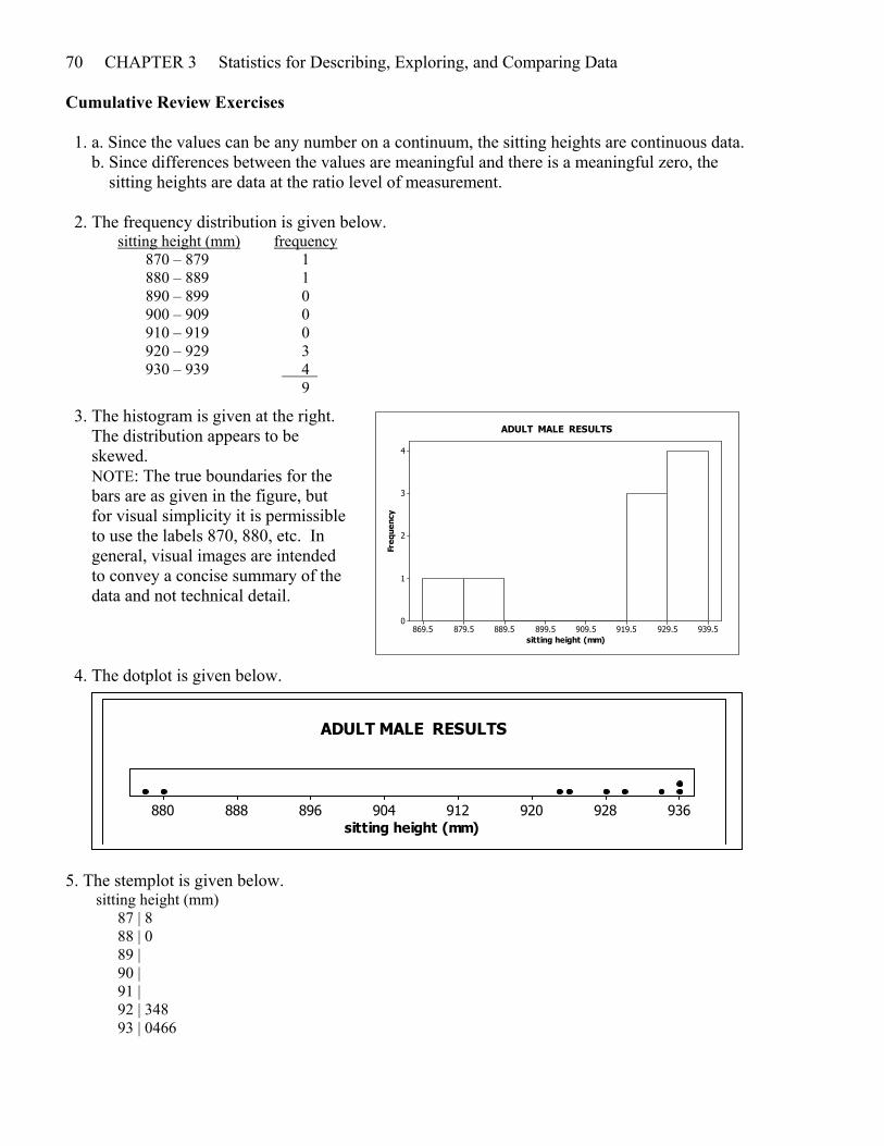
70 CHAPTER 3 Statistics for Describing, Exploring, and Comparing Data Cumulative Review Exercises 1. a. Since the values can be any number on a continuum, the sitting heights are continuous data. b. Since differences between the values are meaningful and there is a meaningful zero, the sitting heights are data at the ratio level of measurement. 2. The frequency distribution is given below. sitting height (mm) frequency 870 – 879 1 880 – 889 1 890 – 899 0 900 – 909 0 910 – 919 0 920 – 929 3 930 – 939 4 . 9

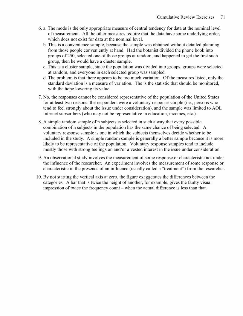
3. The histogram is given at the right. The distribution appears to be skewed. NOTE: The true boundaries for the bars are as given in the figure, but for visual simplicity it is permissible to use the labels 870, 880, etc. In general, visual images are intended to convey a concise summary of the data and not technical detail. 4. The dotplot is given below.

5. The stemplot is given below. sitting height (mm) 87 | 8 88 | 0 89 | 90 | 91 | 92 | 348 93 | 0466

sitting height (mm)

Freq

uenc

y

939.5929.5919.5909.5899.5889.5879.5869.5

4

3

2

1

0

ADULT MALE RESULTS

sitting height (mm)936928920912904896888880

ADULT MALE RESULTS

Cumulative Review Exercises 71 6. a. The mode is the only appropriate measure of central tendency for data at the nominal level of measurement. All the other measures require that the data have some underlying order, which does not exist for data at the nominal level. b. This is a convenience sample, because the sample was obtained without detailed planning from those people conveniently at hand. Had the botanist divided the phone book into groups of 250, selected one of those groups at random, and happened to get the first such group, then he would have a cluster sample. c. This is a cluster sample, since the population was divided into groups, groups were selected at random, and everyone in each selected group was sampled. d. The problem is that there appears to be too much variation. Of the measures listed, only the standard deviation is a measure of variation. The is the statistic that should be monitored, with the hope lowering its value.

7. No, the responses cannot be considered representative of the population of the United States for at least two reasons: the responders were a voluntary response sample (i.e., persons who tend to feel strongly about the issue under consideration), and the sample was limited to AOL Internet subscribers (who may not be representative in education, incomes, etc.).

8. A simple random sample of n subjects is selected in such a way that every possible combination of n subjects in the population has the same chance of being selected. A voluntary response sample is one in which the subjects themselves decide whether to be included in the study. A simple random sample is generally a better sample because it is more likely to be representative of the population. Voluntary response samples tend to include mostly those with strong feelings on and/or a vested interest in the issue under consideration.

9. An observational study involves the measurement of some response or characteristic not under the influence of the researcher. An experiment involves the measurement of some response or characteristic in the presence of an influence (usually called a “treatment”) from the researcher.

10. By not starting the vertical axis at zero, the figure exaggerates the differences between the categories. A bar that is twice the height of another, for example, gives the faulty visual impression of twice the frequency count – when the actual difference is less than that.