chapter 3 measuring shareholder value the economic …

CHAPTER 3

MEASURING SHAREHOLDER VALUE THE ECONOMIC WAY -

SUNDRY APPROACHES

3. 1 THE ACCOUNTING MODELS VERSUS THE ECONOMIC MODELS

The previous chapter concluded by shortly pointing out some shortcomings of the

accounting-based methods. Before starting the discussion on the economic-based

models, a more in-depth discussion on the shortcomings of the accounting-based

methods is not only appropriate, but sets the scene for the next two chapters.

3. 1.1 Introduction

In answer to the question of what drives, determines or sets share prices, there are

two competing answers.

The traditional accounting model of valuation contends that share prices are set

when the stock exchange capitalizes a company's earnings per share (EPS) at an

appropriate price/earnings ratio (P/E ratio). The appeal of this accounting model is

its simplicity and apparent precision. The problem, however, is tha~ the P/E ratio

of a company changes all the time, due to possible acquisitions, changes in

accounting policies or as investment opportunities arise (and/or disappear). This

makes EPS a very unreliable measure of value (Stewart 1990:22).

The economic model of valuation holds that share prices are determined in essence

by just two things: the cash to be generated over the life of a business and the risk

associated with the cash receipts.

The accounting model relies on two distinct financial statements (the income

statement and the balance sheet), whereas the economic model uses only sources

and uses of cash. Whether a cash outlay is included in the income statement or

41

capitalized in the balance sheet makes a big difference to the earnings amount

reported. In the economic model. where cash flows are recorded makes no

difference, unless that affects taxes.

This conflict is further highlighted if a company is permitted to choose between

alternative accounting methods. In other words, there are a number of factors

where different accounting bases are recognised and which can have a substantial

influence on the financial results in the financial statements. The following are

examples:

a) the depreciation of fixed assets;

b) the amortization of intangible assets like research and development, goodwill

and patents;

c) inventory;

d) long-term contracts;

e) deferred tax;

f) instalment transactions;

g) the conversion of foreign exchange;

h) consolidation policies;

i) property development transactions; and

j) product- and service guarantees.

42

These are not the only factors that can give rise to a different treatment of financial

(accounting) data by accountants, as the list can be extended depending on the

specific operations of a company (Vorster, Joubert & Koen 1 996:S-24). A number

of these factors are discussed below.

3.1.2 Inventory valuation - LIFO versus FIFO

In South Africa , a company is permitted to use either the Ll FO (last in, first out) or

FIFO (first in, first out) method of valuating inventory for accounting purposes. The

company is, however, compelled to disclose the valuation on the FIFO basis. If

a company , in a period of rising prices, switches from FIFO to LIFO, the switch will

cause reported earnings to decrease, but the savingjn taxes will cause an increase

in cash. Stewart (1990 24) quotes research that shows that the market focuses

on the increase in cash and not on the decline in book earnings.

An appraiser using accounting-based methods can be faced with earnings per share

(EPS) on the "FIFO" or the "LIFO" method.

3.1.3 The amortization of goodwill

Goodwill can arise when one company acquires another company for a value or

premium over the es timated b ook va lue of t he se ller's asset s.

The amortizat ion of goodwill in the accounting framework reduces reported

earnings. However, b eca use this is a non - cash, non - tax -deducti ble expen se , th e

amorti zation of goodwill per se does not have an influence on th e economic model

of va luation.

Evidence shows th at share prices a re determined by the cash that is expected to

be generated and no t by reported earnings . A co mpany 's earnings expl ain its share

price only t o the extent that earnings reflect the cas h embod ied in the share price

(Stewart 1990 28).

43

3. 1.4 Research and development

Research and development (R & D) is another factor which reveals that earnings

are an inappropriate measure of value.

Accountants can expense R & D outlays as if the potential R & D contribution to

value is applicable only in the accounting period where the expense is incurred.

One of the best examples of how the "misuse" of R & D causes a large

discrepancy between the earnings and book value of a company and its economic

value, is found among companies in the pharmaceutical industry. These companies

spend vast amounts of money on R & D in order to obtain a substantial return over

the long term for their investors. Expensing R & D over a shorter period than the

period over which the expected (cash) benefits will arise is one of the reasons why

these companies' earnings and book values can apparently understate the

companies' value by a large margin. R & D should be capitalized onto the balance

sheet and then amortized against earnings over the period of projected payoff from

the successful R & D efforts.

One of the reasons why companies that invest heavily in R & D often enjoy sky

high share price multiples is the fact that their share prices capitalize an expected

future payoff from their R & D. whereas their earnings are charged with an

immediate expense (Stewart 1990: 29).

3.1.5 Deferred tax

The aspects discussed above dealt with distortions that can affect earnings,

therefore the income statement. However, balance sheet items are also subject to

the accountants' mercy.

One of the items worth mentioning at this point is that of deferred tax. The

question can be asked: is the deferred tax reserve which appears on the

company's balance sheet debt or equity? It normally appears to be in a no-man's-

44

land between debt and equity on the balance sheet. Deferred tax is quite rightly

considered by creditors to be a quasi-liability that uses up a company's capacity to

borrow (Stewart 1990:33).

The entire character of the deferred tax reserve changes if one looks at it from the

viewpoint of the shareholders. As long as the company remains a viable going

concern the company's deferred tax reserve can properly considered to be the

equivalent of common equity and therefore does not have to be separated from net

worth.

Furthermore, the year-to-year change in the reserve ought to be added to retained

profits if the reserve is considered part of shareholders' equity. In this way, taxes

are regarded as an expense only when they are paid (at which time they represents

a cash flow), not when provided for by the accountants.

3. 1.6 Earnings per share and return on net assets (RONA)

Some shortcomings and problems associated with earnings per share (EPS) were

discussed in an example in Section 2.6. It is, however, such an important concept

that it warrants further attention.

Consider an acquisition in which a company selling for a high price earnings (P/E)

ratio buys a firm selling for a low P/E ratio bv exchanging shares. Fewer of the

high P/E shares are needed to retire all the issued low P/E ratio shares. Because

fewer of the high P/E shares (from the buyer) are needed to retire all the issued low

P/E shares, the buyer's EPS will always increase (Stewart 1990:35).

This transaction can also be conducted the other way round, i.e. the low P/E firm

can buy the high-multiple company through a share exchange, in which case the

buyer's EPS will always decrease.

45

Regardless of which company buys and which sells, the "merged company" will

be the same (Hi + Lo = Lo + Hi) with the same assets, prospects, risks, earnings

and value. Accounting earnings, however, suggests that the transaction is

desirable only if it is consummated in one direction, Hi + Lo. In the economic

model, what matters is the exchange of value, and not the exchange of earnings

so popular with accounting enthusiasts.

As mentioned in the previous chapter, earnings growth is also a misleading

indicator of performance. Consider two companies, X andY, which have the same

earnings and the same expected growth rate. The "sameness" would also

probably result in identical share prices and P/E ratios. Suppose that X must invest

more capital than Y to sustain its growth. Y will command a higher share price and

P/E ratio because it earns a higher rate of return on the capital it invests (or, both

companies earn the same, but Y does so on a smaller capital base). X invests to

achieve the growth that Y achieves through a more efficient use of capital.

Rapid growth can be a misleading indicator of added value because it can be

achieved (or "bought") by simply pouring more capital into a business. Earning an

acceptable rate of return on capital invested is essential in the value creation

process. Growth adds to value only when it is accompanied by an adequate rate

of return (Stewart 1990:40).

One of the "fathers" of the economic models of calculating shareholder value, Joel

Stern, wrote as early as 1974 about the dangers of using EPS in an evaluation of

corporate policies.

Apart from his acquisition analysis example set out on the previous page (where

he said that the problem lies in the fact that the pro forma EPS does not determine

the pro forma share price) as discussed above, Stern ( 1974:39) also identified two

other interesting corporate factors where EPS can distort the decision-making

process to the detriment of the shareholders.

46

Firstly, investment should not be confused with financing. There are many ways

in which financing decisions can affect EPS, but investment decisions must be

made independently of financing decisions. Since EPS is calculated by dividing the

net profit attributable to ordinary shareholders by the number of issued shares,

basing investment decisions upon its effect on EPS implies that a specific source

of funds finances a specific use of funds, which is, of course, conceptually

incorrect. EPS can lead the decision-maker to believe that bad investments are

good investments: if he levers (finance) the firm sufficiently at the time the

investment is undertaken, EPS can be manipulated (enhanced) to any level he

desires (Stern 1974:40).

Secondly, an emphasis on EPS can lead to wrong conclusions or decisions about

the proportions of debt and equity in a company's financial structure. Even

though, in most cases, an increase in the amount of debt in relation to equity

enhances EPS, the benefits to a company's share price derived from its financing

policies has nothing to do with EPS. The real benefit of debt financing to ordinary

shareholders is not the added EPS, it is the "government-tax-saving" (own inverted

commas) (Stern 1974:42).

It should be clear at this stage that valuations based on a company's earnings have

many pitfalls and disadvantages. Moreover, to judge by market behaviour, EPS is

not the criterion that impresses the sophisticated investors that really determine

share prices. These investors do not simply discount expected earnings. They

rather discount anticipated cash flows net of the anticipated capital requirements

of the business, the so-called "Free Cash Flow".

The disadvantages of return on equity (ROE) as a method had been discussed in

Chapter 2. One can, however, highlight some other dangers of using this measure

of corporate performance by illustrating what could happen if return on net assets

(RONA) is used as a basis for evaluating and rewarding the managers of the

business.

47

Firstly, if a company or division is currently earning sub-standard returns, managers

can increase RONA by accepting projects with a rate of return higher than RONA,

but is, at the same time, employing a rate which could still be inadequate in the

sense that it could be lower than the cost of capital. These investments, as will

be demonstrated in Chapter 4, reduce shareholder value.

At the other extreme, consider a company that currently earns 25% RONA and has

a cost of capital of 15%. In such a case, a manager could be discouraged from

accepting projects with a rate of return of less than 25% because that would lower

the average RONA. The firm could thus be passing up value-adding investments

(Stern 1994:49).

3. 1. 7 Dividends

3. 1. 7. 1 The theory on dividends

Stewart ( 1990:43) claims that not only do earnings not matter; dividends do not

matter either.

In the economic model of valuation, payment of dividends can be viewed as a sign

that management is unable to find enough attractive investment opportunities to

use all available cash. Once they have distributed attributable earnings in the form

of dividends (instead of re-investing them), management have less capital to fund

future growth opportunities. However, if investment opportunities have been

exhausted, it would be better to pay dividends rather than to make unrewarding

investments.

But what about the shareholders? Do they want dividends? Three theories of

investor preference for dividends can be presented:

a) Miller and Modigliani in Brigham & Gapenski ( 1993:481) argue that dividend

policy is irrelevant; that is, dividend policy does not affect a firm's cost of

48

capital or value. A firm's value is determined by its asset investment policy

and its risk class rather than by how earnings are split between dividends

and retained earnings. These author's propositions were made with a

number of assumptions or conditions, the discussion of which falls beyond

the scope of this study. What is important however is the fact that Miller

and Modigliani argue that a clientele effect exists: a firm will attract

shareholders whose preferences in respect of the payment (quantity or

amount) and stability of dividends correspond to the payment pattern and

stability of the firm itself (Gitman 1994:539). In other words, investors who

seek a certain cash income from their portfolio tend to hold shares which

provide them with that income (a certain dividend amount), or they must

invest in financial instruments which provide them with that desired income.

Investors who need cash do not need to get it from every component of

their portfolio. Investors who prefer capital gains instead, are attracted to

growing firms which entertain a relatively large reinvestment rate. Since

shareholders get what they expect, Miller and Modigliani argue that the

value of a firm's stock is unaffected by its dividend policy. As long as there

are a sufficient number of investors with sufficient income who are seeking

capital gains instead, firms with a relatively low dividend payout ratio need

not worry: their firm's shares will sell for their fair value, unaffected by the

dividend thereon (Stewart 1990:54).

b) Gordon and Lintner in Brigham & Gapenski ( 1993:482) disagree with Miller

and Modigliani and argue that dividends are less risky than capital gains.

Therefore firms should set high dividend payout ratios in order to maximize

their value. Miller and Modigliani disagree, and claim that a bird in the hand

(a dividend) is worth two in the bush (capital gains). Stewart (1990:53)

argues that dividends paid mean certain capital gains lost. Dividends are in

effect "subtracted" from the share price, never to be recouped. The

dividends that are paid out can only make the residual capital gain more

risky.

49

c) Litzenberger and Ramaswamy in Brigham & Gapenski ( 1993:483) bring the

tax effect into the debate. They argue that since dividends attract a higher

tax rate than capital gains (which was the position in South Africa a number

of years ago, but could change in the (near?) future), a firm should pay a low

(or zero) dividend in order to maximize its value. This argument contrasts,

of course, with Gordon and Lintner's theory, but complement the general

viewpoint that dividends do not matter.

One can conclude by stating that it appears that there is just a correlation between

dividend announcements and share price, but not a true causal relationship. It is

helpful to turn to empirical evidence and research in order to see whether these

support the arguments in favour of the economic models.

3. 1. 7. 2 The evidence on dividends

One of the most decisive empirical studies conducted on the effects of dividend

yield and dividend policy on share prices, was done in 1974 by Black and Scholes

(Brigham & Gapenski 1993:483). Their analysis revealed that return to investors

was explained by the level of risk of the firm and not by the dividend payout ratio.

The shares in their sample were classified in different risk classes, and within these

risk classes some shares paid low, some paid modest and some paid high

dividends. All the shares, however, experienced the same rate of return over a

period of time.

The following two important conclusions can be drawn from this study

(Stewart 1990:55):

a) investors should ignore dividends when they are choosing shares. Instead,

they should consider factors like risk, tax and value; and

b) corporate managers should not attempt to influence share prices, investors'

wealth or returns by their dividend policy. They should set a dividend policy

50

within the context of the company's investment programme and financing

policy; that is, a "residual dividend policy", where the first priority is to take

care of all the acceptable investment opportunities, after which the residual

(if any) of the attributable earnings can be distributed as dividends.

3.1.8 Concluding remarks

Earnings, earnings per share and earnings growth are misleading measures of

corporate performance or shareholder wealth. The problem arises from the fact

that earnings can (and must) be altered by means of book entries that have nothing

to do with cash flow.

Value-building investments such as R & D are charged against earnings instead of

taking the real earning power of the expected life span into consideration.

Paying out dividends may deprive worthwhile capital projects of capital or may

force the company and its investors to incur unnecessary transaction costs.

Despite the impressive empirical evidence assembled in the academic community

in favour of the economic model of value, many corporate managers, valuers and

even investors still prefer accounting-based methods (often with earnings as the

basis) in order to determine wealth created for the shareholders of a company.

3.2 INTRODUCTION TO THE ECONOMIC MODELS

During the past three decades there has been a school of writers that have steadily

began to realize the shortcomings of measures such as earnings per share, return

on assets and return on investment.

These traditional measures of company performance are inadequate for the job in

the sense that none of them isolate the most important concern of shareholders:

Is management adding or subtracting value from capital? There has to be a better

51

way.

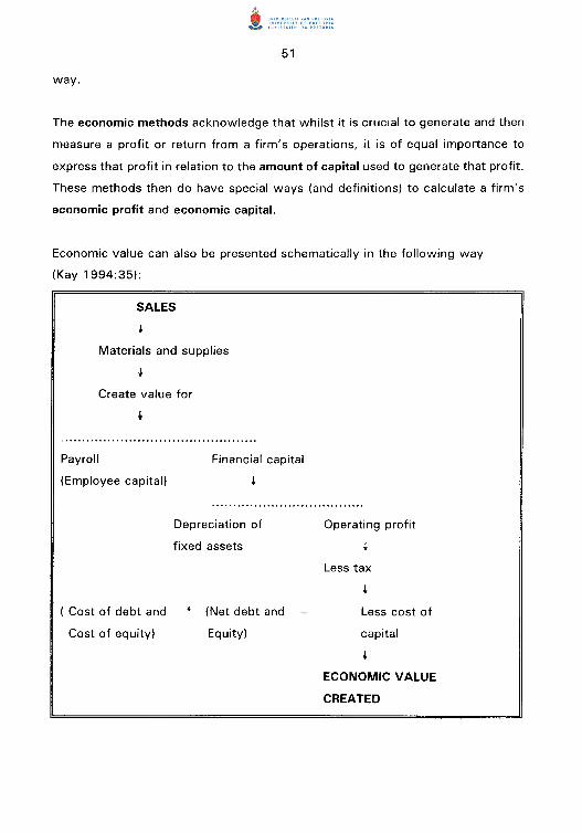
The economic methods acknowledge that whilst it is crucial to generate and then

measure a profit or return from a firm's operations, it is of equal importance to

express that profit in relation to the amount of capital used to generate that profit.

These methods then do have special ways (and definitions) to calculate a firm's

economic profit and economic capital.

Economic value can also be presented schematically in the following way

(Kay 1994:35):

SALES

Materials and supplies

Create value for

Payroll

(Employee capital)

( Cost of debt and

Cost of equity)

Financial capital

Depreciation of

fixed assets

(Net debt and

Equity)

Operating profit

Less tax

Less cost of

capital

ECONOMIC VALUE

CREATED

52

This chapter contains a discussion of a number of sundry economic-based methods

to determine shareholder value.

The build-up to the ultimate model begins with a discussion of the work of Fruhan

(1979). A number of economic valuation-based principles were introduced by him.

The main criticism of his work was that he used only return on equity, and not the

return on total economic capital.

Another author that proposed an economic-based method was Rappaport ( 1 981,

1986). His articles during the early 1980's were followed by his book towards the

end of that decade.

By now, this new way of calculating shareholder value was well established and

Copeland, Koller and Murrin ( 1990) called their method "the economic profit

model".

3.3 USING ECONOMIC VALUE TO MEASURE SHAREHOLDER WEALTH -

EARLIER MODELS

3.3.1 Introduction

One of the first writers to recognize that the pure accounting-based methods of

determining shareholder value were not adequate, was Fruhan.

His book, Financial Strategy. Studies in the creation, transfer, and destruction of

shareholder value, in 1979 was among the first to set out a number of principles

regarding the economic method of calculating shareholder wealth.

Fruhan ( 1979:7) stated that managers create economic value for their firm's

shareholders when they undertake investments that produce returns that exceed

the cost of capital. Fruhan ( 1979: 11) identified three factors which determine the

economic value of a firm's equity:

53

a) the size of the percentage point spread projected to be earned on the

common equity over the cost of the firm's common equity;

b) the amount of future investment opportunities which will generate these

excess returns (this is equal to the net profit attributable to ordinary

shareholders); and

c) the number of years for which these returns can be earned before returns

will be driven down to the cost of equity.

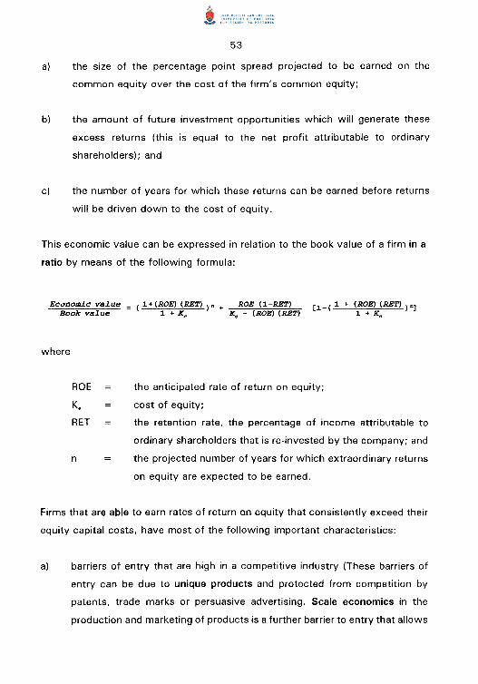
This economic value can be expressed in relation to the book value of a firm in a

ratio by means of the following formula:

Economic value ( 1+(ROE) (RET) )n + ROE (1-RET) [ 1 -( 1 + (ROE) (RET) )n] - Book value 1 + K, K, - (ROE) (RET) 1 + K.,

where

ROE the anticipated rate of return on equity;

Ke cost of equity;

RET the retention rate, the percentage of income attributable to

ordinary shareholders that is re-invested by the company; and

n the projected number of years for which extraordinary returns

on equity are expected to be earned.

Firms that are able to earn rates of return on equity that consistently exceed their

equity capital costs, have most of the following important characteristics:

a) barriers of entry that are high in a competitive industry (These barriers of

entry can be due to unique products and protected from competition by

patents, trade marks or persuasive advertising. Scale economics in the

production and marketing of products is a further barrier to entry that allows

54

a firm a competitive advantage. High capital requirements by certain

industries or firms can also keep competitors at bay);

b) focused product lines and a high market share; and

c) an ability to generate redundant cash, i.e. all cash and marketable securities

less borrowed money.

3.3.2 Method of calculating shareholder value

Fruhan ( 1979:1 02) demonstrates how to calculate the value created for a

company's shareholders. As only the principles and basic calculation methods are

discussed here, readers who are interested in the detail are referred to Fruhan's

work.

Consider the following hypothetical example. A company's return on equity (after

adjustment for the replacement cost of inventory and fixed assets, and for the

capitalization and amortization of research and development expenditure - a topic

discussed in greater detail later in this chapter) amounts to 18,9%. The real cost

of equity capital amounts to 11 ,0%, which means that the firm achieved a real

return on equity that was 7,9 percentage points in excess of the firm's real cost

of equity capital.

Fruhan then proceeds to show how the elimination of the firm's redundant capital

increases the spread between the real rate of return and the real cost of equity

capital. This data is then used in conjunction with the formula in Section 3.2.1 in

order to calculate the economic-value/book-value ratios (Fruhan 1979:1 04). The

value for the firm's shareholders can be estimated by subtracting the adjusted book

value of the firm's equity from its market value.

55

3.3.3 Evaluation

Fruhan did pioneering work in recognizing that there must be as wide as possible

a spread between the return that a firm generates on the invested capital and the

cost of that capital. However, he still uses return on equity in his explanations and

calculations. This is done for both the "return" and the "cost" aspects. It is

demonstrated in the next few sections of this chapter that it is return on invested

capital and the weighted average cost of capital that matters.

The primary objective of Fruhan's work was to demonstrate that thinking about

methods to enhance shareholder value can produce significant benefits for

shareholders. Nevertheless, no checklist designed to ensure enhanced performance

for every firm emerged from his work. None was promised. The work posed a

challenge to managers to consider carefully how they might conduct a systematic

review of value enhancement opportunities.

Management should take into consideration the following factors when thinking

about value enhancement:

a) ability to command premium product prices - in order to increase profit;

b) achievement of a lower than average cost structure - in order to increase

profit;

c) the ability to obtain debt and equity at lower than normal cost - in order to

reduce the financing cost;

d) the design of a capital structure that is more efficient than those of

competitors - in order to reduce financing cost and to optimise the amount

of equity; and

e) the avoidance of actions which may result in value destruction.

56

3.4 SHAREHOLDER VALUE CREATION

3.4.1 Introduction

Another writer who recognised the shortcomings or limitations of the accounting

based methods was Rappaport ( 1981 : 140).

His "shareholder value approach" estimates the economic value of an investment

by discounting the forecast cash flows by the cost of capital. He then goes on to

calculate the present value of a business by discounting the anticipated after-tax

operating cash flow by the weighted average cost of capital.

The next section demonstrates how he incorporates his so-called "value drivers"

(sales growth rate, operating profit margin, income tax rate, capital investment and

a time span) into his shareholder value calculations. The net result of these

calculations is an absolute Rand value which indicates the present value increase

in shareholder value.

3.4.2 The shareholder value approach to a business

As mentioned in Section 3.3.1, any investment's value can be determined by

discounting the anticipated cash flows by the cost of capital.

While many companies use this discounted cash flow (DCF) analysis at project

level, they fail to take the broader picture, that of the entire business (unit), into

consideration. One can thus find a situation where capital projects regularly exceed

the minimum acceptable rate of return, while the business unit itself creates little

or no value for the shareholders (Rappaport 1981:141 ).

In order to extend the DCF approach to the entire business unit, the following

sequential steps must be followed:

57

a) calculate the minimum pretax operating return on incremental sales which

is needed to create value for the business unit (or the entire company);

b) compare the minimum acceptable rates of return on incremental sales with

the rates realised historically and the rates predicted for the future;

c) calculate the contribution to shareholder value of various alternative

strategies; and

d) evaluate the corporate objectives regarding anticipated growth on sales,

capital investments, target capital structure and dividend policy in order to

determine the best value-contributing strategy.

The fourth step above is the subject of both Chapter 5 and the Conclusion to this

study. An example in Section 3.4.3 below illustrates how the first three steps are

calculated.

3.4.3 Calculation of shareholder value created

3. 4. 3. 1 Basic principles and models

The total economic value of a business is the sum of the values of its debt and

equity.

Corporate value Debt + Shareholder value

The present value of the equity claims or shareholder value is then the value of the

company less the market value of currently outstanding debt. The value of the

equity of a firm that expects no further real growth in sales and expects that annual

increases in costs will be offset against increases in sales prices, can be expressed

by the following formula:

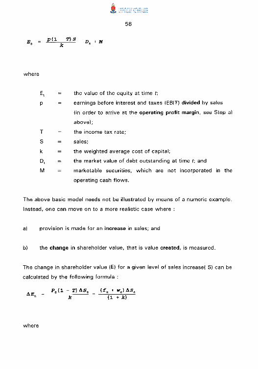
where

p

T

s k

M

58

p(l - T) S _ D + M k t

the value of the equity at time t;

earnings before interest and taxes (EBIT) divided by sales

(in order to arrive at the operating profit margin, see Step a)

above);

the income tax rate;

sales;

the weighted average cost of capital;

the market value of debt outstanding at time t; and

marketable securities, which are not incorporated in the

operating cash flows.

The above basic model needs not be illustrated by means of a numeric example.

Instead, one can move on to a more realistic case where :

a) provision is made for an increase in sales; and

b) the change in shareholder value, that is value created, is measured.

The change in shareholder value (E) for a given level of sales increase( S) can be

calculated by the following formula :

where

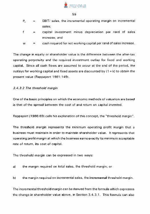
w

59

EBIT I sales, the incremental operating margin on incremental

sales;

capital investment minus depreciation per rand of sales

increase; and

cash required for net working capital per rand of sales increase.

The change in equity or shareholder value is the difference between the after-tax

operating perpetuity and the required investment outlay for fixed and working

capital. Since all cash flows are assumed to occur at the end of the period, the

outlays for working capital and fixed assets are discounted by ( 1 + k) to obtain the

present value (Rappaport 1981: 149).

3. 4. 3. 2 The threshold margin

One of the basic principles on which the economic methods of valuation are based

is that of the spread between the cost of and return on capital invested.

Rappaport ( 1986:69) calls his explanation of this concept, the "threshold margin".

The threshold margin represents the minimum operating profit margin that a

business must maintain in order to maintain shareholder value. It represents that

operating profit margin at which the business earns exactly its minimum acceptable

rate of return, its cost of capital.

The threshold margin can be expressed in two ways:

a) the margin required on total sales, the threshold margin; or

b) the margin required on incremental sales, the incremental threshold margin.

The incremental threshold margin can be derived from the formula which expresses

the change in shareholder value above, in Section 3.4.3.1. This formula can also

60

be expressed in words as follows:

Change in shareholder value

(Present value of incremental cash flow before new investment)

(lncr sales) * (Operating profit margin on incremental sales)

Cost of capital

(Present value of investment in fixed

and working capital)

* (1-T)

(lncr sales) * (Incremental fixed plus working capital rate)

( 1 + Cost of capital)

While the first term represents the present value of the firm's inflows (assumed to

occur from period 1 to perpetuity), the second term represents the present value

of the investment (outflows) necessary to generate these inflows

(Rappaport 1986:72).

There is neither an increase nor a decrease in shareholder value for a specified

sales increase if the value of the inflows is identical to the value of the outflows:

Pt (1 - T)

k

The incremental threshold margin is the operating profit margin on incremental

sales that equates the present value of the cash inflows to the present value of the

outflows. This margin represents the break-even operating return on sales or the

minimum pretax operating return on incremental sales (p'min) needed to create

value for shareholders and is derived as follows (Rappaport 1 981 : 149)

Pmin (£ + w) k

(1 - T) (1 + k)

61

An important fact that emerges from this equation is that when a business is

operating at the threshold margin, sales growth does not create shareholder value.

Shareholder value creation is determined by the product of three factors :

a) sales growth;

b) an incremental threshold spread, that is, profit margin on incremental sales

less the minimum pretax operating return on the incremental sales needed

to create value for shareholders; and

c) the time span of a positive threshold spread (Rappaport 1986:74).

In other words, it is the after-tax capitalized value of the difference between the

minimum acceptable operating return on incremental sales. The change in

shareholder value for time t is then given by the following equation :

(pt - Pt min) (1 - Tt) ASt

k(l + k) t-l

3.4. 3. 3 Calculation example

To illustrate the above principles and formulas as developed by Rappaport, consider

the following hypothetical case:

a) A business forecast the following sales amounts for the next 4 years:

19x0 19x1 19x2 19x3 19x4

Rm 100 115 125 145 160

b) Pretax operating margins on incremental sales amount to 14% for the first

62

2 years after which they will increase to 15%.

c) Working capital per Rand of sales 20%.

d) Capital investment per Rand of sales 30%.

e) Weighted average cost of capital 12%.

f) Tax rate 35%.

Answer

In the first place, the minimum return on incremental sales (P min) must be

calculated, as this input is necessary for the calculation which determines the

increase in shareholder value.

Pmin (:E + w) k

(1 - T) (1 + k)

(0.3 + 0.2) *0.12

0.65*1.12

8.24%

The present value of increase in shareholder value in 19x1 is the following:

<Pt - Pt min) (1 - Tt) liSt

k(1 + k) t-l

(0.14- 0.0824) * (1 - 0.35) * 15

0. 12 * ( 1. 12)0

63

R4,68m

Using the same formula, but applying the relevant inputs as they occur in each year

(pretax operating margin as well as sales change), the present value of increase in

shareholder value is calculated as follows:

19x1 R4,68m

19x2 R2,79m

19x3 R5,84m

19x4 R3.91m

TOTAL R17,22m

To summarise: Over a four year future period, total sales of R545m (with

incremental sales of R60m) will result in a present value increase in shareholder

value of R17 ,22m, taking into consideration the other variables (minimum operating

margin, fixed and working capital levels, the cost of capital and the tax rate) as

specified.


Because this study concentrates on another method of calculating shareholder

value, only a simplified example of the model of Rappaport has been demonstrated.

Interested readers are referred to the work by Rappaport, Creating shareholder

value as indicated above.

This method of calculating the present value of shareholder wealth increase, as

proposed by Rappaport, is actually aimed at a future forecast period, which does

have definite advantages if a new investment strategy and its effects are to be

64

evaluated by management.

However, this method can also be used to calculate the increase in shareholder

wealth in the current year or any other year in the past. All that is needed, of

course, are the relevant inputs in the formulas, which can be obtained from the

(adapted) financial statements.

One of the advantages of this method is its clear indication and identification of the

inputs (value drivers) in the formula in order to determine shareholder wealth (a

topic that is discussed in Chapter 5 of this study).

Although certain variables in the formulas in the example above were kept constant

during the four year period, they can, of course, be varied in order to represent a

more realistic scenario.

The model is easy to use, as well as easy to understand. It is compared and

contrasted with other models at the end of this chapter.

3.5 THE ECONOMIC PROFIT MODEL

3.5.1 Introduction

Copeland, Koller and Murrin (1990:75) also recognise that there are fundamental

problems with the use of accounting-based methods in determining the value of a

company.

They propose a discounted cash flow {DCF) model which calculates the value of

a company by factoring the capital investment and the other cash flows required

to generate the earnings. This approach is based on the principle that an

investment adds value if it generates a return that is higher than returns earned on

investments of similar risk. For a Qiven level of earnings, a company that earns

more on its investments than its competitors can, needs to invest less capital in the

65

business and will generate higher cash flows and higher value.

Valuing a business by determining the present value of its expected cash flows,

leaves unanswered a number of practical questions such as how to determine the

cash flow, investment, or discount rate.

Although these concepts are used in the examples below illustrating these

approaches, a detailed discussion is left for the latter part of this chapter, where

variables that are used as inputs in the models as mentioned, are used in other

models as well.

In this section, firstly certain valuation principles are examined, after which the

Economic Profit Model proposed by Copeland, Koller and Murrin ( 1990: 149) is

illustrated.

3.5.2 Economic valuation principles

The value of a business can be seen as the discounted value of the expected future

free cash flow. Free cash flow is equal to the after tax operating earnings of the

company, plus non-cash charges (for example, the "cost" of depreciation), less

investments in fixed and working capital (Copeland, Koller & Murrin 1990: 139).

Free cash flow excludes any financing-related cash flows such as interest or

dividend payments. These free cash flows are then discounted with the firm's

weighted average cost of capital (WACC) in order to arrive at a present value for

the forecasted period.

However, an additional issue in valuing a business is its infinite life. The value of

the business can be divided over two time periods, namely the value during the

forecast period and the value after the forecasted period.

The value after the forecast period is called the continuing value. There are various

66

methods of calculating the continuing value. One approach is to calculate it as a

perpetuity by means of the following formula:

Net operating profit less adjusted taxes Continuing value

Weighted average cost of capital

The value of a company's debt is deducted from the value of operations as

calculated above. The value of the debt equals the present value of the cash flow

to the debt holders, discounted at a rate that reflects the riskiness of that flow

(Copeland, Koller & Murrin 1990:141). Future borrowing can be ignored, as one

can assume that the inflows from these debts will be equal to the outflows

(repayments).

The above valuation of a company can be illustrated by means of the following

hypothetical example overleaf:

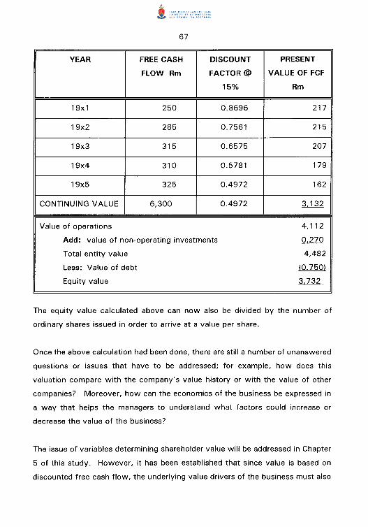
67

YEAR FREE CASH DISCOUNT PRESENT

FLOW Rm FACTOR@ VALUE OF FCF

15% Rm

19x1 250 0.8696 217

19x2 285 0.7561 215

19x3 315 0.6575 207

19x4 310 0.5781 179

19x5 325 0.4972 162

CONTINUING VALUE 6,300 0.4972 3.132

Value of operations 4,112

Add: value of non-operating investments 0,270

Total entity value 4,482

Less: Value of debt (0.750)

Equity value 3.732

The equity value calculated above can now also be divided by the number of

ordinary shares issued in order to arrive at a value per share.

Once the above calculation had been done, there are still a number of unanswered

questions or issues that have to be addressed; for example, how does this

valuation compare with the company's value history or with the value of other

companies? Moreover, how can the economics of the business be expressed in

a way that helps the managers to understand what factors could increase or

decrease the value of the business?

The issue of variables determining shareholder value will be addressed in Chapter

5 of this study. However, it has been established that since value is based on

discounted free cash flow, the underlying value drivers of the business must also

68

be the drivers of free cash flow (Copeland, Koller & Murrin 1990:141 ). The two

key drivers of free cash flow and ultimately value are, firstly, the rate at which a

company can increase its revenues, profits, and capital base, and, secondly, the

return on invested capital. A company that earns higher profits on every Rand

invested than its competitors is worth more than a company that does not have

such a high return. The same applies for a company that grows faster than

another and both earn the same return on invested capital.

It can thus be seen that it is not only the absolute amount of the profit that

matters, but also the amount of capital invested to generate that profit.

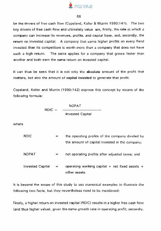
Copeland, Koller and Murrin ( 1990: 142) express this concept by means of the

following formula:

ROIC

where

ROIC

NOPAT

Invested Capital

NOPAT

Invested Capital

the operating profits of the company divided by

the amount of capital invested in the company;

net operating profits after adjusted taxes; and

operating working capital + net fixed assets +

other assets.

It is beyond the scope of this study to use numerical examples to illustrate the

following two facts, but they nevertheless need to be mentioned:

Firstly, a higher return on invested capital (ROIC) results in a higher free cash flow

(and thus higher value), given the same growth rate in operating profit; secondly,

69

an increased growth rate in NOPAT results in lower free cash flows during the

initial years (due to the higher amount of net investment), but later the free cash

flows become much larger and result in greater value.

As long as the return on invested capital (ROIC) is greater than the weighted

average cost of capital (WACC) used to discount the cash flow, higher growth

generates greater value. The core idea is thus that the key drivers of value are

return on invested capital (relative to WACC) and growth (Copeland, Koller &

Murrin (1990: 146).

In Chapter 5 of this study there is a discussion of how these variables must interact

with one another and other variables in order to create value.

3.5.3 The economic profit model

Another model, which Copeland, Koller and Murrin ( 1990: 149) call the Economic

Profit Model, calculates the value of a company by taking the amount of capital

invested and adding to that a premium which represents the present value of the

value created for each future year.

As far back as 1890, Alfred Marshall recognised the concept of economic profit

and stated that the value created by any company must take into account not only

the expenses recorded in the financial statements, but also the opportunity cost of

the capital employed in the business. This means, inter alia, that not only interest

on debt must be accounted for when calculating economic profit, but also the

required rate of return of the ordinary shareholders, which must appear as a "cost"

in the calculations of shareholder value.

One of the advantages of the economic profit model over the discounted cash flow

models is that economic profit is a useful measure for understanding a company's

performance in any single year, while free cash flow is not. One cannot track a

company's progress by comparing actual and projected free cash flow, as this

70

performance of a company is determined by highly discretionary investments in

fixed and working capital. Management could thus easily manipulate investment

decisions (delaying or under-investing) in order to improve free cash flow in a given

year (bearing in mind that free cash flow equals NOPA T less Investment). Such

m3nipulation could be to the detriment of value creation (Copeland, Koller & Murrin

1990:149).

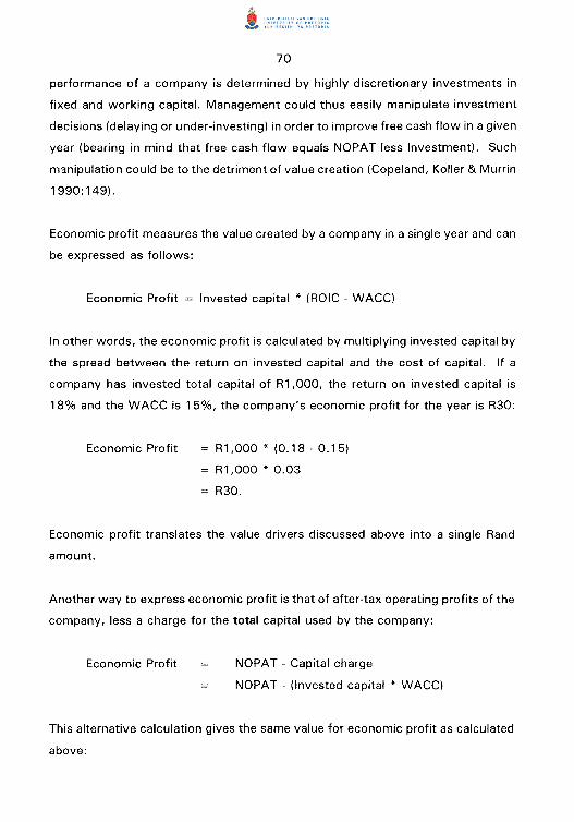
Economic profit measures the value created by a company in a single year and can

be expressed as follows:

Economic Profit Invested capital * (ROIC- WACC)

In other words, the economic profit is calculated by multiplying invested capital by

the spread between the return on invested capital and the cost of capital. If a

company has invested total capital of R1 ,000, the return on invested capital is

18% and the WACC is 15%, the company's economic profit for the year is R30:

Economic Profit R1 ,000 * (0.18- 0.15)

R1 ,000 * 0.03

R30.

Economic profit translates the value drivers discussed above into a single Rand

amount.

Another way to express economic profit is that of after-tax operating profits of the

company, less a charge for the total capital used by the company:

Economic Profit NOPAT- Capital charge

NOPAT- (Invested capital * WACC)

This alternative calculation gives the same value for economic profit as calculated

above:

Economic Profit

71

R 1 80 - ( R 1, 000 * 0. 1 5)

R180- R150

R30.

This approach illustrates the difference between accounting profit and economic

profit: the economic profit takes into account not only the interest on debt, but on

all capital.

A simple example will illustrate how economic profit can be used for valuations.

Assume that the hypothetical company in the example above has invested R 1 000

in working capital and fixed assets in 1 9x 1 . Each year after that, the company

earns R180 in NOPAT (therefore it has a 18% ROIC). If the net investment is

zero, the free cash flow will also be R180 (R180- 0) and the economic profit will

be R30, assuming a WACC of 15%.

The economic profit approach states that the value of a company equals the

amount of capital invested plus the present value of its projected future economic

profit (Copeland, Koller & Murrin 1990: 150).

Value Invested capital + Present value of projected Economic Profit.

If a company earns exactly its WACC during every period (ROIC = WACC), then

the discounted value of its projected free cash flow should equal its invested

capital. In other words, the value of the company is that amount which was

originally invested. The value of a company changes (positively or negatively,

value is added or value is destroyed), if it earns more or less than its WACC

(ROIC > or < WACC).

The value of the company above should equal R 1 000 (its invested capital at the

time of the valuation) plus the present value of its economic profit. Since economic

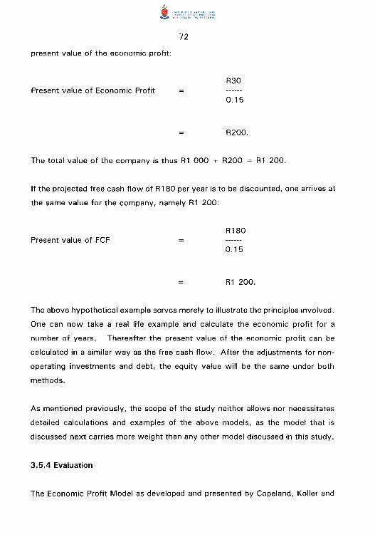
profit remains at R30 to infinity, one can use a perpetuity value to calculate the

72

present value of the economic profit:

Present value of Economic Profit R30

0.15

R200.

The total value of the company is thus R1 000 + R200 R1 200.

If the projected free cash flow of R 180 per year is to be discounted, one arrives at

the same value for the company, namely R1 200:

Present value of FCF R180

0.15

R1 200.

The above hypothetical example serves merely to illustrate the principles involved.

One can now take a real life example and calculate the economic profit for a

number of years. Thereafter the present value of the economic profit can be

calculated in a similar way as the free cash flow. After the adjustments for non

operating investments and debt, the equity value will be the same under both

methods.

As mentioned previously, the scope of the study neither allows nor necessitates

detailed calculations and examples of the above models, as the model that is

discussed next carries more weight than any other model discussed in this study.

3.5.4 Evaluation

The Economic Profit Model as developed and presented by Copeland, Koller and

73

Murrin ( 1990) takes all the principles of economic profit calculation into account.

The model is not only easy to understand, but also give a very clear indication of

value drivers (which are the subject of Chapter 5).

A comparison between models discussed in this chapter will be done at the end of

Chapter 4. A detailed discussion of the last (and in the author's opinion, the best)

model which can be used to calculate the value that a company can create for its

shareholders is set out in Chapter 4.

3.6 CONCLUSION

During the 1970's, Stern started to write about the problems encountered with and

disadvantages of the accounting-based methods. He was a firm believer in the

economic-based methods. It was not, however, until 1986 that his partner,

Stewart, in the consulting firm of Stern Stewart, published a book, The quest for

value, in which his method of determining shareholder value was named

"Economic value added (EVA)".

Although all of the models described above are discussed briefly, EVA is the

method which is concentrated on in this study. It is also used in various ways to

calculate the shareholder value created by management for the owners of a firm.

In the chapters that follow, where the various variables that determine shareholder

value are analyzed, EVA is once again prominent. EVA will be discussed in the

next chapter.

CHAPTER 4

MEASURING SHAREHOLDER VALUE THE ECONOMIC WAY -ECONOMIC VALUE ADDED

4.1 INTRODUCTION

Economic Value Added (EVA) is a measure of corporate performance developed,

refined and popularized by Stern and Stewart of the New York based consulting

firm, Stern Stewart & Co over almost 20 years of working together.

Stern ( 1994:46) admits that the financial concepts which underlie EVA were, of

course, not invented at Stern Stewart & Co. Economists since Adam Smith have

concluded that the goal of any firm and its managers should be to maximize the

firm's value for its owners. Nobel laureate Merton Miller refocused this goal as the

goal of maximizing Net Present Value (NPV). Whilst NPV is primarily a long-term

capital budgeting tool, EVA is an attempt to break this concept down into annual

(or even monthly) instalments which can be used to evaluate the performance of

corporate managers and their businesses.

Most companies use discounted cash flow analysis for capital budgeting

evaluations, but, when it comes to measuring overall corporate performance and

communicating with investors, companies use measures such as earnings, earnings

per share, return on equity (ROE) and the like (Stern 1994:51 ).

The "Du Pont Formula" or return on investment (ROI) is used by many companies

when they wish to evaluate operating performance and capital expenditure. The

ROI calculation can be broken down into more manageable components such as

profit margins, sales turnover and then these components are analyzed even

further. The outcome of this Du Pont analysis has been a proliferation of financial

measures.

Why is it important to have only one measure? Corporate managers in large listed

companies can acquire more capital in order to spend and grow the empire.

75

Internal competition for capital - where different yardsticks are used in the

evaluation - then arises in the company. There are no real trustworthy financial

management system which provides consistent results constantly for operating

heads to choose only those projects that will increase value (Stern 1994:52).

An EVA financial management system is designed to eliminate the above problem.

EVA is a financial management system. It is a framework for all aspects of

financial decision-making that are anchored by an incentive compensation plan.

4.2 CONCEPTS UNDERLYING EVA

Corporate managers have capital provided by the owners of the business at their

disposal. Capital is a scarce resource and therefore it should be assigned to those

undertakings that offer the highest returns. To increase the company's share price,

managers must earn rates of return on capital that exceed the returns offered by

other companies. In this way, they add value to the capital, which is often

reflected in the share price.

Of the factors that account for a company's market value and that are discussed

in detail in Chapter 5, two factors (which flow from the discussion in Chapter 3

above) stand out. These two, the relation between the rate of return and the cost

of capital, often account for a large portion of a company's market value (Stewart

1990:71 ). This now raises the question: What is the best way to measure a

company's rate of return?

Some problems with regard to return on equity (ROE) have been discussed in

Chapter 2. In addition, ROE is based on the same accounting earnings (with all

their problems, disadvantages and distortions) as discussed in Section 3.1.

EVA adjusts reported accounting earnings to eliminate distortions encountered

when measuring true economic performance. Stewart ( 1994:73) states that, in

defining and redefining the EVA measure, a total of 164 performance measurement

76

factors, including methods of addressing shortcomings in conventional General

Accepted Accounting Practice (GAAP) accounting, has been identified. These

factors include those addressed in Section 3.1 of this study. No single company

is likely to encounter all 164 factors. In practice as few as five to ten key

adjustments are actually made. Adjustments can be made only in those cases that

meet four criteria:

a) Is it likely to have a material impact on EVA?

b) Can the managers influence the outcome?

c) Can the operating people understand it?

d) Is the required information relatively easy to track or derive?

The point is that, for any one company, the definition and calculation of EVA is

highly customized in order to strike a practical balance between simplicity and

precision (Stewart 1994: 74).

4.2.1 The rate of return on total capital

Instead of using ROE, the rate of return on total capital can be used as the

yardstick to assess corporate performance. This can be computed by dividing a

firm's net operating profit after taxes (NOPAT) by total capital employed in the

business. This may now be compared directly with the company's cost of capital

in order to determine whether value is being created or destroyed

(Stewart 1990:86).

NOPAT

capital

Capital is the sum of all cash invested in the business over time and in any form or

by any name whatsoever. NOPAT is the profit derived from operations, after tax,

but before financing charges (interest, dividends) and other non-cash items (e.g.

depreciation).

77

The rate of return on capital may be computed either from a financing or from an

operating perspective. Because ofthe importance of EVA in this study, both these

methods are discussed below in Section 4.2.2 and Section 4.2.3.

4.2.3 The rate of return from a financing perspective

The rate of return (r) is, from a financing perspective, free from any distortions

which debt (leverage) can inflict upon the standard ROE.

Consider the following calculation of the rate of return:

NOPAT

capital

where

NOPAT

Capital

Income attributable to ordinary shareholders

+ Interest payments after tax savings

Common equity

+ Debt

The NOPAT return on capital is what the return on equity would be, assuming that

only equity financing has been employed (Stewart 1990:87). The return (r) is thus

free from any financial leverage actions. The benefit of debt manifests itself in the

weighted average cost of capital (c) against which the return (r) is compared.

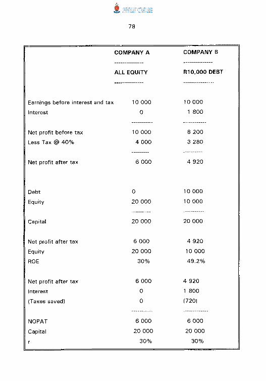
In order to illustrate this important principle, consider the following hypothetical

example:

Earnings before interest and tax

Interest

Net profit before tax

Less Tax@ 40%

Net profit after tax

Debt

Equity

Capital


Equity

ROE


Interest

(Taxes saved)

NOPAT

Capital

78

COMPANY A

ALL EQUITY

10 000

0

10 000

4 000

6 000

0

20 000

20 000

6 000

20 000

30%

6 000

0

0

-----------

6 000

20 000

30%

COMPANY B

R10,000 DEBT

10 000

1 800

8 200

3 280

4 920

10 000

10 000

-----------

20 000

4 920

10 000

49.2%

4 920

1 800

(720)

-------------

6 000

20 000

30%

79

As can be seen in the above example, NOPAT, as well as NOPAT return on capital

(r), remains unchanged by leverage. What matters is the amount of capital

employed, and not in what form that capital has been obtained.

The next step to improve the rate of return is to eliminate other financing

distortions. This is done by taking into account preferred shareholders interest as

well as minority investors.

NOPAT

capital

where

NOPAT

and

Capital


+ Preferred dividend

+ Minority interest provision


Common equity

+ Preferred share capital

+ Minority interest

+ Debt

Note that for every adjustment to NOPAT, there is a corresponding adjustment to

capital. The NOPAT as calculated above is the amount available to all providers of

capital to the business (Stewart 1990:90).

80

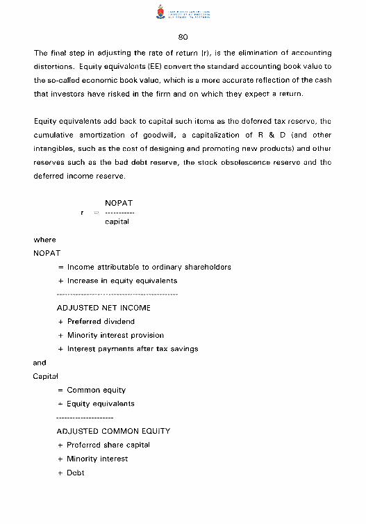
The final step in adjusting the rate of return (r), is the elimination of accounting

distortions. Equity equivalents (EE) convert the standard accounting book value to

the so-called economic book value, which is a more accurate reflection of the cash

that investors have risked in the firm and on which they expect a return.

Equity equivalents add back to capital such items as the deferred tax reserve, the

cumulative amortization of goodwill, a capitalization of R & D (and other

intangibles, such as the cost of designing and promoting new products) and other

reserves such as the bad debt reserve, the stock obsolescence reserve and the

deferred income reserve.

NOPAT

capital

where

NOPAT


+ Increase in equity equivalents

ADJUSTED NET INCOME

+ Preferred dividend

and

Capital

+ Minority interest provision


Common equity

+ Equity equivalents

ADJUSTED COMMON EQUITY

+ Preferred share capital

+ Minority interest

+ Debt

81

With the incorporation of equity equivalents into capital and NOPA T, the rate of

return is an even more accurate indication of the yield earned by all the capital

providers of the business.

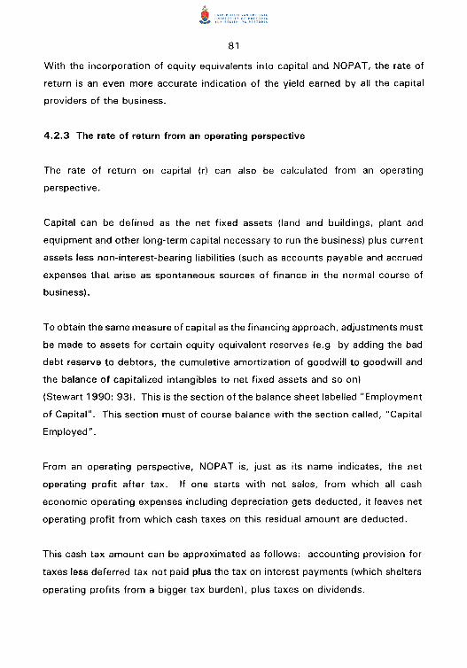
4.2.3 The rate of return from an operating perspective

The rate of return on capital (r) can also be calculated from an operating

perspective.

Capital can be defined as the net fixed assets (land and buildings, plant and

equipment and other long-term capital necessary to run the business) plus current

assets less non-interest-bearing liabilities (such as accounts payable and accrued

expenses that arise as spontaneous sources of finance in the normal course of

business).

To obtain the same measure of capital as the financing approach, adjustments must

be made to assets for certain equity equivalent reserves (e.g by adding the bad

debt reserve to debtors, the cumulative amortization of goodwill to goodwill and

the balance of capitalized intangibles to net fixed assets and so on)

(Stewart 1990: 93). This is the section of the balance sheet labelled "Employment

of Capital". This section must of course balance with the section called, "Capital

Employed".

From an operating perspective, NOPAT is, just as its name indicates, the net

operating profit after tax. If one starts with net sales, from which all cash

economic operating expenses including depreciation gets deducted, it leaves net

operating profit from which cash taxes on this residual amount are deducted.

This cash tax amount can be approximated as follows: accounting provision for

taxes less deferred tax not paid plus the tax on interest payments (which shelters

operating profits from a bigger tax burden), plus taxes on dividends.

NOPAT

capital

where

NOPAT

Sales

- Operating expenses

-Taxes

and

Capital

Net working capital

+ Net fixed assets


82

A business that wants to add value to the capital it employs for its shareholders

(investors), must earn a rate of return that exceeds the cost of capital of the

business.

Measures such as ROE are a flawed measure of performance, due to distortions

resulting from accounting conventions that make financial statements more useful

for lenders than for shareholders.

The rate of return on total capital should be used to measure corporate

performance. This can be obtained by dividing NOPAT by the capital employed in

operations. Stewart ( 1990: 111) called this an "after-tax cash-on-cash" yield

earned in the business. It is a measure of the productivity of the capital employed

in the business, irrespective of the method of financing used and free from

accounting distortions arising from accrual bookkeeping entries.

83

It is the relationship between this rate of return (r) and the cost of capital that

forms one of the EVA method.

4.3 EVA DEFINED

4.3. 1 The theoretical model

As can be deducted from the introductory discussion above on the principles

underlying EVA, in essence, EVA is a way of measuring the economic value

(profitability) of a business after the total cost of capital - both debt and equity -

has been taken into account. One must remember that most traditional

(accounting-based) methods take only debt into account. The calculation of EVA

also includes the often considerable cost of equity (Firer 1995:57).

The main shortcomings of other methods have been dealt with briefly. The key

principle of EVA is that value is created when the return on an investment exceeds

the total cost of capital that correctly reflects its investment risk. One can improve

EVA (and thus shareholder value) as long as one accepts new projects on which

the rate of return exceeds the cost thereof.

EVA is an internal performance measure of a company's operations on a year-to

year basis. It reflects the successes of the efforts of corporate managers to add

value to the shareholders' investment.

EVA is the residual income left over from the operating profits after the total cost

of capital has been subtracted. A positive EVA implies that the rate of return on

capital must exceed the required rate of return. To the extent that a company's

EVA is greater than zero, the firm is creating (adding) value for its shareholders

(Stern 1994:49).

EVA is a kind of annual instalment of the multi-year Net Present Value (NPV) that

is calculated by using the standard discounted cash flow capital (DCF) budgeting

84

technique. The similarity between EVA and NPV lies in the fact that they both

measure the degree to which a firm is successful in earning a rate of return that

exceeds the cost of capital It is, however, demonstrated later in this chapter that

EVA is a far better tool for the job than NPV or DCF, even though these methods,

if properly applied, result in the same answers over an extended period of time.

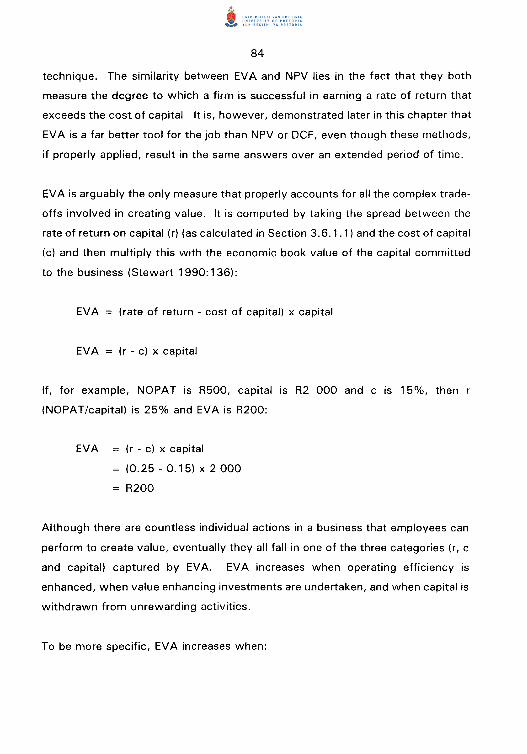
EVA is arguably the only measure that properly accounts for all the complex trade

offs involved in creating value. It is computed by taking the spread between the

rate of return on capital (r) (as calculated in Section 3. 6.1. 1) and the cost of capital

(c) and then multiply this with the economic book value of the capital committed

to the business (Stewart 1990: 136):

EVA (rate of return - cost of capital) x capital

EVA (r - c) x capital

If, for example, NOPAT is R500, capital is R2 000 and c is 15%, then r

(NOPAT/capital) is 25% and EVA is R200:


(0.25 - 0.15) X 2 000

R200

Although there are countless individual actions in a business that employees can

perform to create value, eventually they all fall in one of the three categories (r, c

and capital) captured by EVA. EVA increases when operating efficiency is

enhanced, when value enhancing investments are undertaken, and when capital is

withdrawn from unrewarding activities.

To be more specific, EVA increases when:

85

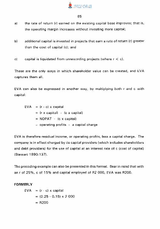
a) the rate of return (r) earned on the existing capital base improves; that is,

the operating margin increases without investing more capital;

b) additional capital is invested in projects that earn a rate of return (r) greater

than the cost of capital (c); and

c) capital is liquidated from unrew2rding projects (where r < c).

These are the only ways in which shareholder value can be created, and EVA

captures them all.

EVA can also be expressed in another way, by multiplying both r and c with

capital:


(r x capital) - (c x capital)

NOPAT - (c x capital)

operating profits - a capital charge

EVA is therefore residual income, or operating profits, less a capital charge. The

company is in effect charged by its capital providers (which includes shareholders

and debt providers) for the use of capital at an interest rate of c (cost of capital)

(Stewart 1990: 137).

The preceding example can also be presented in this format. Bear in mind that with

an r of 25%, c of 15% and capital employed of R2 000, EVA was R200.

FORMERLY


( 0. 2 5 - 0. 1 5) X 2 000

R200

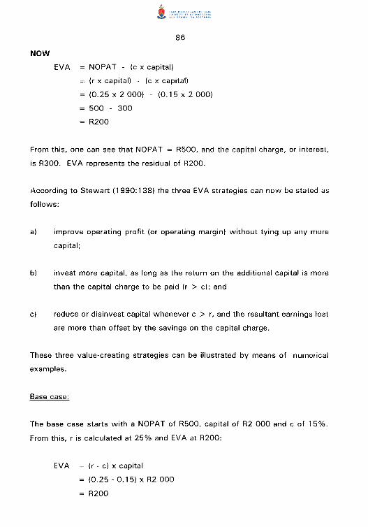
NOW

86

EVA NOPAT - (c x capital)

(r x capital) - (c x capital)

(0.25 X 2 000) - (0.15 X 2 000)

500 - 300

R200

From this, one can see that NOPAT = R500, and the capital charge, or interest,

is R300. EVA represents the residual of R200.

According to Stewart ( 1 990: 1 38) the three EVA strategies can now be stated as

follows:

a) improve operating profit (or operating margin) without tying up any more

capital;

b) invest more capital, as long as the return on the additional capital is more

than the capital charge to be paid (r > c); and

c) reduce or disinvest capital whenever c > r, and the resultant earnings lost

are more than offset by the savings on the capital charge.

These three value-creating strategies can be illustrated by means of numerical

examples.

Base case:

The base case starts with a NOPAT of R500, capital of R2 000 and c of 15%.

From this, r is calculated at 25% and EVA at R200:


(0.25 - 0.15) X R2 000

R200

87

Value-creating strategy (a): Improve operating efficiency

NOPAT increases to, say, R600 due to administrative savings or greater efficiency

in the production process. Then r increases to 30% ( R600/R2 000), and EVA

increases to R300:


(0.30 - 0.15) X R2 000

R300

Value-creating strategy (b): Achieve a profitable investment

A proposed new project requires a capital investment of R 1 000 and is expected

to earn a rate of return of 20% and thereby adding R200 to NOPAT. In this case,

r is 23% (R700/R3 000) and EVA increases to R21 0:


(0.23 - 0.15) X R3 000

R210

Note in this case that although the rate of return decreases from 25% to 23%,

EVA increases from R200 to R21 0.

Value-creating strategy (c): Rationalize and curtail unproductive investments

(c)( 1 l Liquidate unproductive capital

R500 of excess working capital can be withdrawn from business operations

without affecting NOPAT. This causes the rate of return to increase to 33%

(R500/R2 OOO-R500) and EVA to R270:


(0.33- 0.15) x R1 500

R270

88

(c)(2) Curtail investment in unrewarding projects

Start with a completely new case. Assume that a company earns a NOPAT of

R200 on R2 000 capital. With a return of only 1 0%, EVA is negative R 1 00:


(0.10- 0.15) X R2 000

= -R1 00

Suppose now that the company has the opportunity to undertake a new project

with a capital investment of R1 000 and a return of 13%, therefore adding R130

to NOPAT. The consolidated return increases to 11% (R330/R3 000) but EVA

declines further, to negative R 120:


(0.11 - 0.15) X R3 000

= -R120

Although the rate of return increases, more value is destroyed for the shareholders.

In addition to the above cases, another value-creating option for a firm is

mentioned briefly.

Value-creating strategy : Changing the cost of capital (c)

Starting with the first base case again, suppose that the company is able to

substitute some of its high cost capital for lower cost capital (by increasing its debt

ratio). This results in an interest bill saving of, say, R50 and a reduction inc to,

89

say, 12%. NOPAT now drops (remember that NOPAT = attributable income +

interest expense after tax, and therefore a lower interest bill will lower NOPAT)

with R50 x ( 1-Tax rate), say, a total of R30. The rate of return is now 24%

((R500-R30)/R2,000)) and EVA increases to R240:


(0.24- 0.12) x R2 000

R240

These calculations demonstrate how the EVA of a company can be determined, as

well as how changes in the three inputs in the formula bring about a change in the

value created or value destroyed.

However, EVA must at this stage be put to another test. If EVA is a good

performance measure, it ought to be able to set apart or distinguish between the

value-creation efforts of competing companies.

Consider the following cases of Companies A, B and C:

A B

(r- c) 15%-15%17.5%-15%

x increase in Capital R1 000 R 800

Incremental EVA R 0 R 20

c

17.5%-15%

R2000

R 50

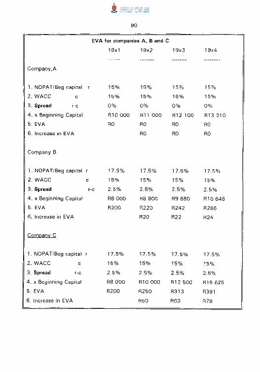
These calculations can now be presented on a more detailed year-to-year basis in

order to illustrate the principle of an ongoing EVA calculation and comparison

between companies:

90

EVA for companies A, B and C

19x1 19x2 19x3 19x4

Company A

1. NOPAT/Beg capital r 15% 15% 15% 15%

2. WACC c 15% 15% 15% 15%

3. Spread r-c 0% 0% 0% 0%

4. x Beginning Capital R1 0 000 R11 000 R12 100 R13 310

5. EVA RO RO RO RO

6. Increase in EVA RO RO RO

Company B

1. NOPAT/Beg capital r 17.5% 17.5% 17.5% 17.5%

2. WACC c 15% 15% 15% 15%

3. Spread r-c 2.5% 2.5% 2.5% 2.5%

4. x Beginning Capital R8 000 R8 800 R9 680 R10 648

5. EVA R200 R220 R242 R266

6. Increase in EVA R20 R22 R24

Company C

1. NOPAT/Beg capital r 17.5% 17.5% 17.5% 17.5°/o

2. WACC c 15% 15% 15% 15%

3. Spread r-c 2.5% 2.5% 2.5% 2.5%

4. x Beginning Capital R8 000 R1 0 000 R12 500 R15 625

5. EVA R200 R250 R313 R391

6. Increase in EVA R50 R63 R78

91

EVA is obtained by multiplying the spread between rand c by the capital invested.

Incremental EVA is determined by the increase in EVA, or the r- c spread multiplied

by the increase in capital.

Various scenarios have been presented above to illustrate the calculation of EVA.

The possibilities are by no means exhausted and are dealt with in more detail in

Chapter 5 of this study, which concentrates on the variables determining EVA.

At this stage, it should be clear that the EVA valuation procedure is not a far

fetched new method or theory of valuation; it is just a form of the discounted cash

flow method. It is a mathematical truism that, for a given forecast, the value

determined by discounting projected EVA and adding it to the current capital

balance, equals the value computed by discounting the anticipated free cash flow

to a present value (Stewart 1990: 175).

The above hypothetical examples were used in conjunction with the theoretical

principles to demonstrate the basic mechanics of Economic Value Added as a

valuation and performance measurement tool.

One can now develop and expand the EVA method by introducing present value

discounting into the process.

4.3.2 Explanatory calculations

The EVA valuation method calculates how much value has been and will be created

(or destroyed). When a company's EVA is projected and discounted to a present

value, EVA accounts for the market value that management has added or

subtracted from the capital at its disposal:

Value Capital + Present Value of all future EVA

92

Value is calculated in three steps. Firstly, the annual EVA-values are discounted

to the present value. Secondly, one must provide for the period beyond the time

span (T) under review. This is done by capitalizing the NOPAT achieved in the first

year after T as a perpetuity and then discounting it to the present. Lastly, one

adds current capital (in year 0, the beginning of the valuation period) to the

discounted EVA values.

Normal capital budgeting techniques often assume that cash flows occur at the end

of the period, and therefore do not adjust the discount factor or the cash flows for

re-investing the cash flows at any time throughout the year. However, it makes

more sense to assume that the cash flows that occur during the year can be re

invested at some rate.

For the purposes of the example below midyear discounting is used at the cost of

capital and the discount factor is adjusted accordingly. This implies that the capital

at the beginning of the period must be adjusted to midyear by adding half a year's

interest at the cost of capital rate (discount rate).

93

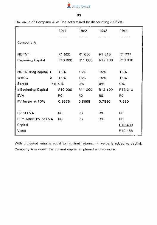
The value of Company A will be determined by discounting its EVA:

19x1 19x2 19x3 19x4

,!:ompany A

NOPAT R1 500 R1 650 R1 815 R1 997

Beginning Capital R10 000 R11 000 R12 100 R13 310

NOPAT/Beg capital r 15% 15% 15% 15%

WACC c 15% 15% 15% 15%

Spread r-c 0% 0% 0% 0%

x Beginning Capital R10 000 R11 000 R12 100 R13310

EVA RO RO RO RO

PV factor at 1 0% 0.9535 0.8668 0.7880 7.880

PV of EVA RO RO RO RO

Cumulative PV of EVA RO RO RO RO

Capital R1 0 488

Value R1 0 488

With projected returns equal to required returns, no value is added to capital.

Company A is worth the current capital employed and no more.

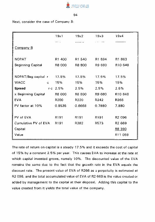
94

Next, consider the case of Company B:

19x1 19x2 19x3 19x4

Company B

NOPAT R1 400 R1 540 R1 694 R1 863

Beginning Capital R8 000 R8 800 R9 680 R1 0 648

NOPAT/Beg capital r 17.5% 17.5% 17.5% 17.5%

WACC c 15% 15% 15% 15%

Spread r-c 2.5% 2.5% 2.5% 2.5%

x Beginning Capital R8 000 R8 800 R9 680 R1 0 648

EVA R200 R220 R242 R266

PV factor at 10% 0.9535 0.8668 0.7880 7.880

PV of EVA R191 R191 R191 R2 096

Cumulative PV of EVA R191 R382 R573 R2 669

Capital R8 390

Value R11 059

The rate of return on capital is a steady 1 7. 5% and it exceeds the cost of capital

of 1 5% by a constant 2. 5% per year. This causes EVA to increase at the rate. at

which capital invested grows, namely 10%. The discounted value of the EVA

remains the same due to the fact that the growth rate in the EVA equals the

discount rate. The present value of EVA of R266 as a perpetuity is estimated at

R2 096, and the total accumulated value of EVA of R2 669 is the value created or

added by management to the capital at their disposal. Adding this capital to the

value created from it yields the total value of the company.

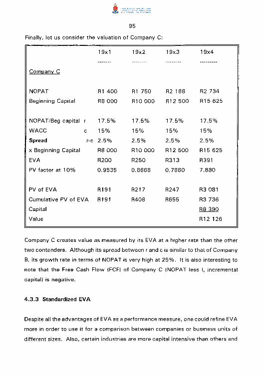
95

Finally, let us consider the valuation of Company C:

19x1 19x2 19x3 19x4

Company C

NOPAT R1 400 R1 750 R2 188 R2 734

Beginning Capital R8 000 R1 0 000 R12 500 R15 625

NOPAT/Beg capital r 17.5% 17.5% 17.5% 17.5%

WACC c 15% 15% 15% 15%

Spread r-c 2.5% 2.5% 2.5% 2.5%

x Beginning Capital R8 000 R10 000 R12 500 R15 625

EVA R200 R250 R313 R391

PV factor at 1 0% 0.9535 0.8668 0.7880 7.880

PV of EVA R191 R217 R247 R3 081

Cumulative PV of EVA R191 R408 R655 R3 736

Capital R8 390

Value R12 126

Company C creates value as measured by its EVA at a higher rate than the other

two contenders. Although its spread between rand c is similar to that of Company

B, its growth rate in terms of NOPAT is very high at 25%. It is also interesting to

note that the Free Cash Flow (FCF) of Company C (NOPAT less I, incremental

capital) is negative.

4.3.3 Standardized EVA

Despite all the advantages of EVA as a performance measure, one could refine EVA

more in order to use it for a comparison between companies or business units of

different sizes. Also, certain industries are more capital intensive than others and

96

there is a need for a common basis for comparison. EVA can be standardized to

reflect a common level of capital employed.

In order to standardize EVA, the capital employed needs to be standardized to a

base year. The spread (r- c) is not affected by the scaling. The capital employed

in the first year is divided by itself (the base year capital employed) and multiplied

by 100. Thus, the standardized EVA in the first year of the analysis is always

equal to the spread between that year's r and c multiplied by 100.

In the second year of analysis, that year's capital employed is divided by the base

year's capital employed, multiplied by 100 and multiplied in turn by the spread in

order to attain the standardized EVA of the second year. This process is repeated

for every year for the entire period under review.

Standardized EVA increases if the spread (r - c) is increased, new capital is

invested productively, or if capital is withdrawn from uneconomical activities.

Shortcomings, distinctions and comparisons between companies show up more

clearly when EVA is standardized in this way. These characteristics are utilized in

the empirical part of this study.


A detailed evaluation of EVA as a performance measure is done at the end of this

chapter. However, at this stage, after the above hypothetical examples, one can

mantion a number of features of this model.

In the first place, EVA reduces all the ways in which a company can create value

to only three: Measuring the efficiency of current operating activities, taking

profitable growth into consideration and eliminating uneconomical activities (both

in terms of operating and capital investment).

97

Secondly, when projected and discounted to a present value, EVA represents the

net present value of all past and projected capital projects. Thus, maximizing EVA

as a company objective is not only compatible with the overall goal of the firm, but

such a step will ensure that the share price continues to grow as the stock market

price exceeds the capital investment in the firm.

Although EVA yields the same value as discounting the free cash flow, EVA as a

measure is better in the sense that it connects forward-looking valuation

procedures with an evaluation of performance (Stewart 1990: 178).

4.4 MARKET VALUE ADDED

4.4. 1 Introduction

Market value added (MVA) was also developed at the Stern Stewart consultancy

firm. Although this is another method of determining the value of a company, it

is dealt with under the heading of EVA, as there is a close relationship between

these two concepts.

Companies can be ranked according to how much value they have added to, or

subtracted from, their shareholder investment. Market value added is the

difference between a company's fair market value, as reflected primarily in its share

price, and the economic book value of capital employed. Readers are at this stage

reminded of the difference between the economic book value and the accounting

book value, as discussed in Sections 3.1 and 3.2 above, as well as in Chapter 2.

The economic book value is bound to be considerably larger than the accounting

book value as indicated in the annual financial statements. Besides the

conventional book equity (share capital, share premium, retained earnings and

reserves) it also includes equity equivalent reserves (bad debt and LIFO reserves,

the capitalization of R&D and deferred tax to name but a few) to provide a more

accurate indication of the shareholders' total cash investment in the company

(Stewart 1990 : 180).

98

The concept of market value added can be expressed in a simple formula:

Market value added market value - capital

If a company has a market value of R500m, but has capital to the worth of R600m

invested, it has a negative MVA of R1 OOm. However, if the same company only

had R300m in invested capital, the managers of the company would have added

R200m in value to the investors' capital at their disposal.

From the above, one can deduce that a company's MVA is the share market's

assessment, at any given time, of how successfully the company has invested its

capital in the past and how successfully investors expect the capital to be invested

in future. Maximizing a company's MVA is thus synonymous to maximizing

shareholder value, which is the goal of the firm.

MVA can also be calculated by multiplying the number of shares issued by the

difference between the market price of the shares and the economic book value of

the shares:

MVA = number of shares * (market price- economic book value per share)

= share market value - economic book value (capital)

The economic book value consists of the economic capital as we defined it for the

purposes of calculating a company's EVA. Adding equity equivalents to capital,

adjusts MVA for the many distortions that can cause an overstatement of value

created by capital intensive, high-tech or risky companies. These factors may be

discounted in the share price at the left hand side of the above equation, and,

unless is accounted for, on the other side of the formula, value (MVA) will also be

overstated.

It is also important to note that it is not total value (market capitalization, the first

term in the MV A calculation) that counts. This would be an incomplete

99

measurement of corporate performance, as it does not take into consideration the

amount of capital used to create that value. A company can increase its total value

by investing more capital (both by retaining earnings and raising new capital in

whatever form). The efficient use of the shareholder's capital can only be

measured according to net present values - that is, the total value less the total

capital used, or the increase in value, less the additional new capital invested in the

business (Stewart 1990: 190).

Changes in the levels of MV A over a given period are bound to be as useful (if not

more so) than the total levels of MVA itself. An increase in MVA is a sign that a

company is producing higher rates of return on capital than the cost of that capital.

The opposite happens when the return of capital is lower than the cost thereon:

a negative MV A is accorded to a company, its managers and its shareholders.

The above argument indicate the link between EVA and MVA as two valuation

concepts. It is this link that forms the subject of the discussion in the next section.

4.4.2 MVA and EVA

EVA can be viewed as that internal measure of performance that best reflects the

company's success in adding value to the capital invested by shareholders. It is

therefore strongly related to both the level and the changes in MVA over time.

As explained above, EVA is the residual income left over from operating income

after the cost of capital has been deducted. According to Stewart ( 1990: 192),

EVA can also be thought of as the economic earnings that are capitalized by the

market in arriving at a company's MVA. The MVA can therefore be regarded as

the external or "market" measure of performance of a company's success.

However, the link between a company's EVA and MVA goes further. It can, in

fact, be expressed mathematically. A company's market value added at any point

in time is equal to the discounted present value of all the EVA the company is

expected to generate in the future.

100

Thus, companies that earn exactly their cost of capital have an EVA of RO and sell

at a market value equal to capital, and therefore have as MVA zero. Companies

that earn in excess of their cost of capital are rewarded by the market with positive

MVAs (in line with the positive EVAs that can be computed from their results).

MVA

MVA

market value - capital

present value of all future EV As

Stewart ( 1990: 153) describes a company's EVA as the fuel that fires its MVA.

EVA is the internal measure which leads to the external consequence of building

a premium or discount into the market value of a company. Diagrammatically, this

can be expressed as follows:

101

The Relationship Between EVA and MV A

Premium Value

Market

Value

Market

Value

Added

Capital

EVA1 + EVA2

(1 +C*)1 (1 +C*)2

Discounted Value

Capital

Market

Value

Lost

Market

Value

+ •••••••

(EVA1)

(1 +C*)1 +

(EVA2)

(1 +C*)2

It is difficult to illustrate the calculation of a company's MVA by means of a

hypothetical example as key variables also need to be estimated. In the following

section, a real life example is used. However, as a run-up to this, consider the

following illustration which is an extension of the calculations of EVA done in

Section 4.3.1 above:

+

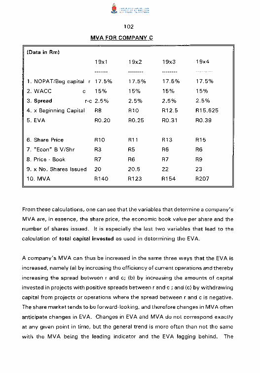
102

MVA FOR COMPANY C

(Data in Rm)

19x1 19x2 19x3 19x4

1. NOPAT/Beg capital r 17.5% 17.5% 17.5% 17.5%

2. WACC c 15% 15% 15% 15%

3. Spread r-c 2.5% 2.5% 2.5% 2.5%

4. x Beginning Capital R8 R10 R12.5 R15.625

5. EVA R0.20 R0.25 R0.31 R0.39

6. Share Price R10 R11 R13 R15

7. "Econ" B V/Shr R3 R5 R6 R6

8. Price - Book R7 R6 R7 R9

9. x No. Shares Issued 20 20.5 22 23

10. MVA R140 R123 R154 R207

From these calculations, one can see that the variables that determine a company's

MVA are, in essence, the share price, the economic book value per share and the

number of shares issued. It is especially the last two variables that lead to the

calculation of total capital invested as used in determining the EVA.

A company's MVA can thus be increased in the same three ways that the EVA is

increased, namely (a) by increasing the efficiency of current operations and thereby

increasing the spread between r and c; (b) by increasing the amounts of capital

invested in projects with positive spreads between rand c; and (c) by withdrawing

capital from projects or operations where the spread between rand cis negative.

The share market tends to be forward-looking, and therefore changes in MV A often

anticipate changes in EVA. Changes in EVA and MVA do not correspond exactly

at any given point in time, but the general trend is more often than not the same

with the MVA being the leading indicator and the EVA lagging behind. The

103

correlation between these two valuation concepts is discussed in Section 4.4.5 of

this study.

4.4.3 Standardized MVA

The MVA can also be standardized and then related to EVA. Stewart ( 1990: 173)

standardizes the number of shares issued on the same principle as capital employed

was standardized in the calculation of standardized EVA.

The actual number of shares issued is divided by the capital employed at the end

of the first year (the base figure) and then multiplied by 1 00. This adjusted

(standardised) amount of shares issued is multiplied by the difference between the

market value and the book value per share in order to arrive at the standardized

MVA.

In the second year, the actual number of shares issued is once again divided by the

capital employed at the end of the first year, then multiplied by 100 to arrive at the

standardized number of shares issued, and the rest of the calculations are

completed to obtain the standardized MVA.

Note that in standardizing EVA, capital employed at the beginning of the first year

is used, whilst in standardizing MVA, it is the capital at the end of the period that

is used. The reason for this is twofold. Firstly, it takes time for capital to become

fully productive and, secondly, MVA is calculated using the share price as it is

reflected at the end of the year.

Standardized MVA is utilized extensively in the empirical part of this study.

4.4.4 The 0-ratio

There is another method very similar to the MVA method, namely the Q ratio. This

ratio was developed in the 1960s by Nobel Prize winning economist James Tobin.

104

The ratio is calculated by adding the market value of a company's equity (both

ordinary and preference shares), debt and other long-term liabilities together. This

is expressed against the current value of the company's asset base (comprised of

the net assets and working capital, adjusted for inflation) (Ryan 1994: 16).

Companies with a ratio greater than one have been able to add value to the assets

under their control, while those with a, atio of less than one have destroyed value.

Companies can improve their ratio by good asset management (for example by

reducing stock levels), rationalisation (of both assets, costs or product range),

restructuring and cost containment in order to improve margins.

From the above one can see the similarities with EVA and MV A more clearly. The

same factors that influence EVA also come into play with the 0 ratio. Stewart

( 1 990: 181), in elaborating on MV A, states that he focuses on the market value of

a company's total debt and equity in relation to the capital employed in assets

(though no mention is made of whether assets are adjusted for inflation or not).

Managers are really managers of assets and not of equity.

This study, however, concentrates, inter alia, on MV A as a measure of shareholder

wealth.


MVA is the absolute Rand spread between a company's market value and total

capital invested. Unlike a rate of return, which reflects the outcome of one period,

MVA is a cumulative measure of corporate performance. It is the wealth created

by management over and above the total resources invested. MVA can also be

regarded as the market's assessment of the quality of management (Stern 1994:

43).

105

The close relationship between a company's EVA and MV A originates from the fact

that these measures are based on the same underlying principles, concepts and

amounts. MVA, which is forward-looking, is closely associated with historical EVA.

If managers strive to maximize a company's EVA, MV A automatically follows, as

does the improvement in shareholder value. Maximizing MVA should be the

primary objective for the management of a company that is concerned about its

shareholders' wealth (Stewart 1990: 153).

4.5 EVA CALCULATION OF SASOL (LTD).

As an example, a calculation of the EVA of Sasol L TO is presented overleaf:

106

ECONOMIC VALUE ADDED (EVA) (1992/1993)

1. RETURN ON CAPITAL EMPLOYED CROCE)

Net Operating Profit after Tax (NOPA 1) X 100 Beginning Capital

1 614 X 100 19 987

8.1%

2. SPREAD

REFER NOTE

Return on Capital employed - Weighted Average Cost of Capital 5*

ROCE- WACC

8,1 - 18,1

3. ECONOMIC VALUE ADDED (EVA)

Beginning Capital x Spread

R19 987 million x (10%)

R 1 998 million Shortfall

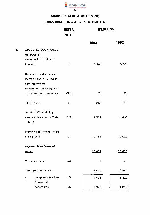
107

MARKET VALUE ADDED (MVA)

(1992/1993- FINANCIAL STATEMENTS)

REFER R'MILLION

NOTE

1993 1992

1. ADJUSTED BOOK VALUE

OF EQUITY

Ordinary Shareholders'

Interest 6 781 5 961

Cumulative extraordinary

loss/gain (Note 17 - Cash

flow statement:

Adjustment for loss/(profit)

on disposal of fixed assets) CFS (3) (2)

Ll FO reserve 2 343 311

Goodwill (Coal Mining

assets at book value (Refer B/S 1 582 1 403

note 1)

Inflation adjustment - other

fixed assets 3 10 758 8 929

Adjusted Book Value of

equity 19 461 16 602

Minority interest B/S 91 76

Total long-term capital 2 520 2 850

Long-term liabilities B/S Q Q Convertible

debentures B/S 8 8

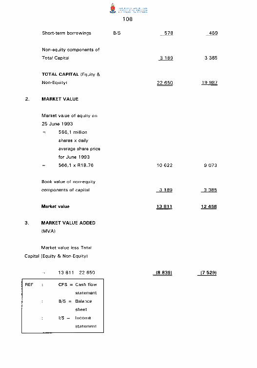
108

Short-term borrowings B/S ~ 459

Non-equity components of

Total Capital 3 189 3 385

TOTAL CAPITAL (Equity &

Non-Equity) 22 650 19 987

2. MARKET VALUE

Market value of equity on

25 June 1993

566,1 million

shares x daily

average share price

for June 1993

566,1 x R18,76 10 622 9 073

Book value of non-equity

components of capital 3 189 3 385

Market value 13 811 12 458

3. MARKET VALUE ADDED

(MVA)

Market value less Total

Capital (Equity & Non-Equity)

13 811-22 650 (8 839) (7 5291

REF CFS = Cash flow

statement

B/S Balance

sheet

1/S Income

statement

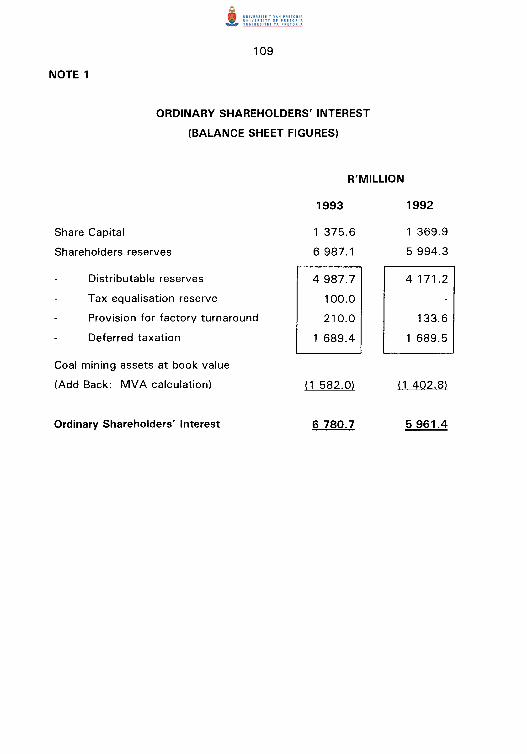
NOTE 1

109

ORDINARY SHAREHOLDERS' INTEREST

(BALANCE SHEET FIGURES)

R'MILLION

Share Capital

Shareholders reserves

Distributable reserves

Tax equalisation reserve

Provision for factory turnaround

Deferred taxation

Coal mining assets at book value

(Add Back: MV A calculation)

Ordinary Shareholders' Interest

1993

1 375.6

6 987.1

4 987.7

100.0

210.0

1 689.4

( 1 582.0)

6 780.7

1992

1 369.9

5 994.3

4 171.2

133.6

1 689.5

(1 402.8)

5 961.4

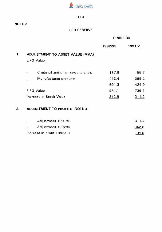
110

NOTE 2

LIFO RESERVE

1. ADJUSTMENT TO ASSET VALUE (MVA)

LIFO Value

Crude oil and other raw materials

Manufactured products

FIFO Value

Increase in Stock Value

2. ADJUSTMENT TO PROFITS (NOTE 4)

Adjustment 1991/92

Adjustment 1992/93

Increase in profit 1992/93

R'MILLION

1992/93

137.9

453.4

591.3

934.1

342.8

1991/2

55.7

369.2

424.9

736.1

311.2

311.2

342.8

31.6

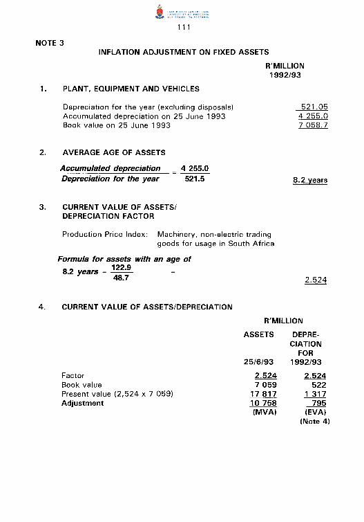
111

NOTE 3 INFLATION ADJUSTMENT ON FIXED ASSETS

R'MILLION 1992/93

1. PLANT, EQUIPMENT AND VEHICLES

Depreciation for the year (excluding disposals) Accumulated depreciation on 25 June 1 993 Book value on 25 June 1 993

2. AVERAGE AGE OF ASSETS

Accumulated depreciation Depreciation for the year

3. CURRENT VALUE OF ASSETS/ DEPRECIATION FACTOR

4 255.0 521.5

Production Price Index: Machinery, non-electric trading goods for usage in South Africa

Formula for assets with an age of

8.2 years = 122·9 48.7

4. CURRENT VALUE OF ASSETS/DEPRECIATION

521.05 4 255.0 7 058.7

8.2 years

R'MILLION

Factor Book value Present value (2,524 x 7 059) Adjustment

ASSETS

25/6/93

2.524 7 059

17 817 10 758 (MVA)

DEPRECIATION

FOR 1992/93

2.524 522

1 317 795

(EVA) (Note 4)

NOTE 4

112

NET OPERATING INCOME AFTER TAX (NOPAT)

REFER R'MILLION

1. ADJUSTED EBIT-CALCULATION Net income before taxation Plus: Interest paid

Loans Convertible debentures

LIFO adjustment

Less: Depreciation adjustment Plus: Holding Gain Adjusted EBIT

2. CASH INCOME TAX Taxation per income statement Tax saving on convertible debenture interest Net taxation for the year per income statement Taxation on interest paid Taxation on extra ordinary items Cash tax

3. NET OPERATING PROFIT AFTER TAX Adjusted EBIT Cash tax NOPAT (EVA)

NOTE

1/S

1/S I

1/S

2

3 7

6

1 835.9 439.0

350.3 88.7

_ll,_Q 2 306.5

(794.8) 608.0

2 119.7

347.9 ~ 312.4

(193.2)

505.6

2 120 506

1 614

113

NOTE 5 WEIGHTED AVERAGE COST OF CAPITAL

(WACC)

Equity

Debt

Notes:

1.

3 YEAR AVERAGE DEBT

TO CAPITAL RATIO

85.72

14.28

100.00

Cost of equity

Risk free rate (Government bonds) Estimated risk premium Sasol's beta

2. Cost of debt

Cost of debt is estimated at 50 basis points over the risk free rate

AFTER TAX RETURN

19.76

8.12

After tax cost of debt = 14.5 x 0.56 = Tax rate (Note 6)

( 1)

(2)

WEIGHTED AVERAGE COST

OF CAPITAL

6% 0.96

(WACC) %

16.9

1.2

18.1

%

14.00

114

NOTE 6 TAXATION ON INTEREST PAID (1992/1993)

1. EFFECTIVE TAX RATE

Net income before taxation Taxation @ 40% Taxation on dividends declared (15% of R487) Tax liability

Effective tax rate ___!QI__ x 1 00 M% 1 836 1

2. INTEREST PAID

Interest paid (per income statement) Loans Convertible debentures

3. TAXATION ON INTEREST PAID (NOTE 4)

Interest paid x effective tax rate 439 X 44% = 193.2

R'MILLION

350.3 88.7

439.0

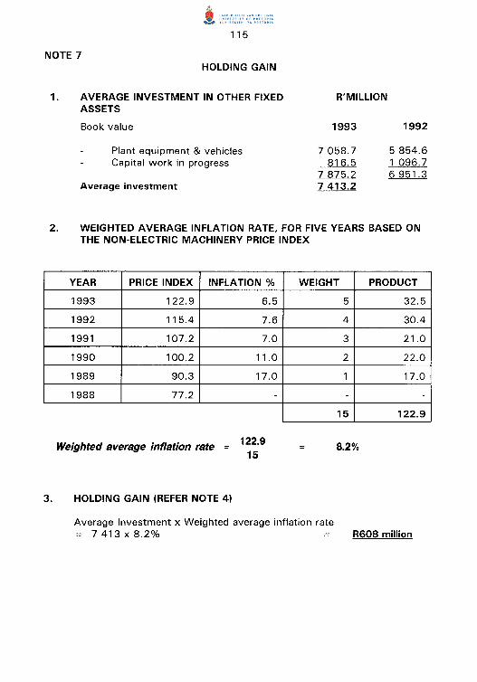
115

NOTE 7

1.

HOLDING GAIN

AVERAGE INVESTMENT IN OTHER FIXED ASSETS

Book value

Plant equipment & vehicles Capital work in progress

Average investment

R'MILLION

1993

7 058.7 816.5

7 875.2 7 413.2

1992

5 854.6 1 096.7 6 951.3

2. WEIGHTED AVERAGE INFLATION RATE, FOR FIVE YEARS BASED ON THE NON-ELECTRIC MACHINERY PRICE INDEX

YEAR PRICE INDEX INFLATION%

1993 122.9

1992 115.4

1991 107.2

1990 100.2

1989 90.3

1988 77.2

Weighted average inflation rate

3. HOLDING GAIN (REFER NOTE 4)

6.5

7.6

7.0

11.0

17.0

122.9 15

-

WEIGHT

5

4

3

2

1

-

15

8.2%

Average Investment x Weighted average inflation rate

PRODUCT

32.5

30.4

21.0

22.0

17.0

-

122.9

= 7 413 x 8.2% R608 million

116

4.5 CRITICISM OF EVA

Although EVA as a measure of corporate performance is the method which the

various variables determining shareholder value in this study are derived from, it

does have a number of shortcomings, as any such a system would have.

Many of the criticisms targeted against EVA are based on misconceptions about

or ignorance of the subject. Other problems with EVA originate from a lack of

management support (for whatever reason), whilst still other problems seem to

have genuine grounds. The various criticisms or problems people have with EVA

will be given simultaneously with explanations and clarification where applicable.

Stewart ( 1995:81 ), one of the fathers of EVA, addresses the five main ways in

which managers err in applying EVA. Firstly, EVA must be a way of life. One must

adopt EVA and not merely calculate it. Secondly, most managers try to implement

EVA too rapidly. Depending on the size, complexity or diversity of the

organization, it could take from five months up to a year to implement EVA,

starting from top management and then gradually pushing it down the ranks.

Thirdly, there must be a process of selling EVA, but it should be sold with the idea

that it is going to be bought by everyone in the organization. All the department

heads must work together, driven by the EVA incentive plan (see Chapter 8 of this

study) in order to make a success of the EVA system. Fourthly, it must be

conveyed to the managers and all other employees that EVA will reward all

stakeholders of the firm if it is correctly implemented. Lastly, the training of all

employees in EVA is important, because even those who do the smallest jobs can

help create value.

Another aspect that can create a problem for the management of a company is the

fact that the share market is forward-looking. When one announces that one is

going to adopt an EVA system, or that one is going to spin off or sell a subsidiary,

the company's share price is likely to go up. Internally, though, one has not

achieved that value yet. One has to spend the next two years or so achieving that

117

expected value just in order to keep the share price from falling. The solution to

this problem is to use EVA as an internal measure of performance and to let MV A

be the barometer of the market's expectations.

Another aspect of EVA that needs careful consideration is that of determining the

cost of capital, or c, as it has been used in the calculations. This is particularly

relevant in decentralized companies with various business units. The weighted

average cost of capital (WACC) is not an output of the accounting system. Sub

optimal shareholder value may arise if the WACC is determined incorrectly (Best

1995:38). Calculating WACC is an important step in the EVA calculation, but what

is more important is the fact that just charging managers for the use of total

capital, and making their bonuses depend to a large extent on covering that capital

charge, goes a longer way towards motivating efficiency than making subtle

distinctions between levels of risk and cost of capital.

If one is going to hold people accountable for their performances on a year-to-year

basis, one has a problem if one has large investments in time period zero whilst

benefits might accrue only in the second, third, etc. years. Glasser (1996:42), the

CEO of a company in the USA (GATX), contends that the EVA approach can

penalize companies that utilize assets with long-term returns. Their investments

generate a regular revenue stream during their life, and a lump sum when they are

sold. The more such companies invest, the lower their EVA. When investments

are restricted, EVA improves. Stern ( 1994: 64) attempts to solve this problem by

putting large capital expenditure items into a suspense account. Instead of being

amortized on a standard depreciation schedule, they bear interest at the required

rate of return. The company and its shareholders thereby avoid being penalized for

investing large sums.

One must also remember that it is possible to get into a situation where a company

can have a negative EVA due to a (continuous) big investment programme, but, if

the returns are attractive (r > c), the market can realize this and the company may

be rewarded accordingly by an increasing MV A. As Stewart ( 1 990: 124) strikingly

puts it: "Happiness is a negative cash flow - so long as the returns are attractive".

118

Stewart ( 1 994: 79) also addresses the issue of depreciation by stating that it

troubles some critics that EVA is measured after subtracting depreciation from the

income statement and the balance sheet. It seems that the basis for confusion is

the notion that depreciation cannot be an economic charge because it is a non-cash

charge. Depreciation is, however, an economic charge, because it is a cash

equivalent charge, in the sense that one pays for depreciation in cash if one leases

the asset instead of owning it. But, taking a steady depreciation charge (straight

line depreciation) against a steady cash flow leaves steady earnings against an

asset base that declines with depreciation. The problem is real, however the culprit

is not EVA, but it is basing depreciation on an accounting basis instead of on an

"economic" basis. One way to address this problem (in addition to the method

mentioned in the paragraph above) is to implement a sinking-fund depreciation

where little depreciation (and thus more earnings) is recorded early on and, more

depreciation (and fewer earnings) towards the end of the project. EVA is therefore

recorded over the life of the asset. In practice, however, one finds that the

distortion is immaterial as long as a company has a reasonably steady capital

spending programme which calls for continuous growth and replacement (Stewart

1994:81).

When a company manufactures a number of products in various divisions, one can

allocate costs down to the cent and they will be right mathematically, but they do

not tell one anything about the true economic profitability of producing a joint

product. Neither EVA nor any other accounting system is set up to handle the kind

of problem that arises from synergies. One can measure the EVA of an entire

company, but when one tries and divide the EVA, one gets the classic "hamburger

and hide" problem of allocating joint costs and benefits. In order to resolve this

problem, one has to revert to some subjective judgement of cost or benefit

allocations by top management.

Staying with the "accounting problems" of EVA, the question of whether EVA is

based upon book values can arise. Stewart ( 1994:78) advances several interesting

explanations for why it is more cost effective to use book values instead of market

119

values when one is calculating EVA. Firstly, adjusting and updating values to

market values on a regular basis sometimes calls for subjectivity, in any case

imposes large costs on any accounting system. Secondly, a way to circumvent the

problem of historical costs has been found: managers can be rewarded, not for the

absolute value of EVA, but for the year-to-year changes in EVA. If one rewards

managers for improving EVA, it does not really matter what value one initially

assign to the assets, because the three principal ways to increase EVA (see Section

4.3.1) have nothing to do with the existing asset base.

For an EVA system to be effective, one has to be willing to decentralize the firm

and "empower" the operating"managers. Not all the decisions can be made at the

top of the organization. The problem that arises is that, in certain industries

(stable, mature, low-tech industries facing no competition), decentralization is

probably not ideal. The agency costs associated with delegating decisions to line

managers in such cases probably outweigh the benefits (Stern 1994:68).

Sheenan ( 1994:86) does not criticise the EVA system per se, but he is doubtful

that EVA is the only answer. The long-term success and survival of a company

depends not only on the shareholders (or their wealth), but also on the benefits

received by other stakeholders in the company. These can include customers,

employees and suppliers of labour, technology and capital. Long-term shareholder

wealth can only prosper when these factors combine in a synergy. EVA is a

valuable tool in setting the right goals and objectives, but reaching those goals

requires more than an inward look at capital, cash flows, cost of capital and

compensation. It is also necessary to be outward-looking, facing customer needs

and meeting customer demands more efficiently than the competition can.

In order for EVA to be successful, a company must ensure that its employees are

inspired to change and head for superior performance, away from their

conventional comfort zone. Sometimes sweeping organizational cultural changes

are needed to ensure that the goals set by EVA can be met, and more often than

not, one finds that convincing and moving employees to do just that can be one

of the major obstacles in the path of the EVA system.

120

4. 7 BENEFITS OF THE EVA SYSTEM

The EVA financial system forms one of the cornerstones of this study, which in

itself could be an indication of the sound principles and advantages thereof.

The discussion, explanations and calculations of EVA above, should make EVA's

advantages obvious. It is, however, appropriate to conclude this section on EVA

with a short summary of EVA's unique advantages over other (economic) models

of determining shareholder value.

EVA encourages managers, in fact all employees of a business, to look for

profitable growth opportunities, while at the same time economizing on the use of

capital. This is particularly relevant (and in fact necessary) in South Africa where

businesses have to contend with high interest rates, and capital is a scarce

resource.

A problem that arises all over the world is that many companies have become too

big and complex to be managed from one central place, and therefore one needs

to decentralize decision-making and controls. Empowerment through organizational

structures means that one has to align the incentives of the operating managers

with those of top management and shareholders. The EVA system can accomplish

all of this, provided that commitment can be obtained from all the parties

concerned.

EVA puts the emphasis in a company's performance on both profits and returns.

Both the quantity and quality dimensions of earnings are taken care of. The right

balance between profitability and growth is struck so that there is not just a push

for ever-increasing revenues without a corresponding check on what it took

(expenses and capital) to generate said revenues.

A strong selling point of EVA as a management tool is that it provides a clear

statement of financial objectives which can be communicated to all levels of

121

management. EVA is also a good way of communicating, not only with

shareholders, but also with institutional investors and analysts. It is an alternative

accounting framework that should encourage more and better communication

between management and shareholders and between shareholders themselves

(Stern 1994:60).

Although the implementation of the EVA system can be difficult, it is important to

remember that it provides, in essence, a simple measure or yardstick. It is the

simplicity of the concept that can make employees in all levels of the company

conscious of what they are doing and why they are doing it. If one rewards people

on a clear and simple basis, one can impress shareholder wealth creation into their

very being. Even if some individuals do not get it right at first, peer pressure alone

should move most to behave as value-maximisers (Stern 1994:70).

In management's quest to manage a company in the best interests of the

shareholders, one often finds that a number of performance measures are being

used which the operating managers must adhere to. EVA is a single measure that

embodies all the aspects of both the efficient application of company resources as

and shareholder wealth creation. With EVA as the basis for capital budgeting

calculations, performance evaluations and bonus determinations, managers tend

to spend money as carefully as though it is their own, with accompanying benefits

for the company and its shareholders (Stewart 1994:74). It comes as no surprise

when, after EVA has been implemented as an operating measure, an "original"

capital expenditure program is trimmed down, and, in some cases, a substantial

reduction takes place. The reason for this is probably that on some extra or

incremental funds, the cost of capital cannot be earned thereby adversely affecting

not only company or division performance, but also the managers' bonuses.

Remember that on performance measures such as return on investment, return on

assets or earnings, investment projects can look attractive whilst they actually

destroy wealth.

122

Managers of a company can have different goals from that of the shareholders of

the firm. This conflict of interests is described as the agency theory (Jensen &

Meckling 1976:305). A number of managerial incentives have been developed over

the years in order to bridge this gap between the goals of managers and

shareholders. These incentives include cash bonuses, performance shares and

employee share option plans. It falls beyond the scope of this study to debate the

merits of the different incentive schemes or even other possible solutions.

However, it is relevant to this study that EVA provides shareholders with a solution

to the agency problem. Whilst it is widely recognised that some form of incentive

or reward (of whatever nature) is necessary to persuade managers to act in the

best interests of shareholders, it is the performance measures utilised to determine

the rewards of the managers that are under scrutiny. In the past, measures such

as earnings per share, return on equity, sales or even years of service with the

company were used. EVA provides a perfect solution to this problem, and, in fact,

an increasing number of companies are implementing an employee reward system

based on EVA, together with the EVA system itself. Managers are now rewarded

if they increase shareholder wealth as measured by EVA.

Sheehan ( 1994:86) elaborates on the above ideas and states that actions such as

those as described in the paragraph above attempt to reduce the agency problem

by motivating managers to feel like business owners. Some economic rationality

is found in some successful private companies that was not always present in

public companies. Owners of private companies do not invest in projects with a

negative return, nor do they manage their companies for accounting profits. Often

one sees public companies undertake initiatives designed to increase short-term

accounting earnings while reducing cash or economic returns.

Likewise, one seldom hears the owner of a private company saying that equity

funding is "cheap", let alone ignoring a return thereon when tallying up the past

year's financial performance. Equity capital is extremely valuable to a private

owner. Managers who have little or no shareholding in the company and are

compensated on a cash basis often do not see the sense of these arguments,

123

which demonstrates the existence of the agency problem in a slightly different

form. A reward system based on EVA can change all of this.

Another sector where EVA can be applied with success is in the state or semi-state

institutions. Stern ( 1 994: 70) describes the implementation of EVA at a

government agency in South Africa a number of years ago. Four months were

spent implementing the programme and conveying its contents, meaning, principles

and goals to the more than 11 000 employees, 85% of whom did not have a

matric. The programme was such a success that the EVA for the first six months

exceeded five times the forecast for the entire year. There are however, a number

of conditions which must be met and unique problems which must be overcome

when one targets the semi-state sector. Firstly, there must be a measurable capital

base as well as income or turnover (expenses are usually no problem). Secondly,

determining the cost of capital, and more specifically the cost of equity, could be

a thorny issue, although with certain assumptions these problems can be

overcome. The moral of the story, however, remains that, in many cases, all one

has to do to improve people's performance is to get them to understand how

superior performance can help themselves.

To illustrate the above point, one can consider the fact that EVA is to be

jmplemented at the United States Postal Service (Spinner 1995:93). The U.S.

Postal Service had losses in 18 of the last 25 years. If the EVA programme is

successful, the Postal Service could generate up to $1 billion toward the end of the

century. It is a capital-starved, labour-intensive, highly regulated government

institution. Furthermore, faxes, e-mail and the advent of electronic banking

threaten to make inroads into the traditional fields of services provided by the

Postal Services. From a financial perspective, the Postal Service operates under

constraints that would frustrate most private-sector financial executives. It does

not have access to a bank line of credit; it must borrow at a rate most large

corporations would not consider favourable. The Postal Service is also tied down

by Senate and by public opinion. The reader can probably draw the parallels and

see the similarities between the U.S. Postal Service and the South African post

124

office. Everything fits, especially the huge losses reported lately. Is it possible to

implement EVA in such a scenario? Moreover, what are the chances of bringing

about a positive change? Let us briefly consider this real test for EVA's

capabilities.

In order to implement the EVA programme in an institution with characteristics

such as those of the postal services, one needs to develop a method to calculate

the contributions by various local offices or clusters of offices accurately and to

reward employees for improvements. To measure whether a given cluster is adding

value or not, a new method of allocating revenues must be developed. Revenues

are usually allocated independently of the labour required to produce them. For

example, the postage revenue from bulk-mail catalogues or accounts are received

by one post office while other offices must do the actual processing, distribution

and delivery.

Tc solve such problems and make it possible to generate meaningful EVA figures,

the U.S. Postal Service developed a system of transfer pricing based on statistical

analysis of samples of mail from various locations. These statistics can be

accurate down to the cluster level. By allocating costs and revenues according to

work load, employees' energies can be directed in more productively.

Whilst it can be difficult to calculate and allocate revenues as described above, an

even more difficult issue can be that of determining the cost of capital, and more

particularly the cost of equity. In the case of the U.S. Postal Service, it was

decided to charge each performance cluster for capital, plant, machines, trucks,

offices etc. at 12% (Spinner 1995:95). It was calculated that after deducting a

cost of capital of 12%, break-even occurs, which in itself is a monumental

achievement. Stewart himself said in one of Stern's articles (Stern 1994: 64) that

when people ask him these days what the cost of capital is, he often tells them

that it is 12%, because that is 1% per month. From this statement it should be

clear where, one year later, the U.S. Postal Service derived their 12% cost of

capital from. Recall also that in Section 3.6.5 above it was stated that just

125

charging managers for the use of capital motivates them and improves their

efficiency. In the case of the postal services, the aim is to keep costs down and

to provide quality service to the customers.

Furthermore, the head of the U.S. Postal Service recognises that EVA brings

together all aspects of one business into one measure. It changes the focus from

the traditional government culture. Revenues can be increased only when it is

profitable, investment can take place only when it produces a return in excess of

the cost of capital and costs can be reduced only when it does not impede on

service to customers.

From the above, it can be seen that EVA's application and advantages can be

stretched beyond the traditional (listed) companies. Semi-government institutions,

and in South Africa's case, the postal services, can also reap the benefits of the

EVA system or at least from applying its principles.

To conclude this section, one can say that EVA and its underlying "building blocks"

are a dependable statement of performance, because the measure is free from the

limitations of the nature and rules of accounting data. Comparability is made

possible between divisions and between organisations. One can even go further

and say that EVA provides global uniformity relating to the valuation and

interpretation of shareholder wealth (Best 1995:38).

4.8 CONCLUSION

The last section of this chapter gives a brief "different" overview of Chapters 2, 3

and 4 in order to set the scene for the following chapter. Apart from illustrating

how the evolution of (financial) management causes the need to arise for a

different way of measuring shareholder value, attention is also given to a concept

that has not been previously discussed, but which has played (and sometimes still

does play) an important role in this whole process, namely the leveraged buy-out

(LBO) that was so popular a number of years ago.

126

In the end, EVA proves to be not only the answer to many problems, but also

overcomes many obstacles. It can also be used to analyse the variables or pillars

on which it is built.

4.8.1 Evolution

With the ever-increasing change in technology and the information associated with

that change, together with the rise of a global economy, brought about

considerable changes in the structure and control systems of large companies.

Centrally-directed economies are failing and state-owned enterprises all over the

world are increasingly being privatised.

This change is also accompanied by a flattening of management hierarchies, with

the responsibility for corporate decision-making being driven down the ranks to

managers and employees closer to the company's operations and customers (Stern,

Stewart & Chew 1995:32).

One of the questions or problems that now arises is that of correct decision-making

and distinguishing between not only profitable or unprofitable capital investment

projects, but any decision that may affect the wealth of shareholders. Is there an

(accounting) system that can provide the correct answer at the time when the

decision has to be made?

The answer lies, of course, not with a computer or accounting system of some

sort, but with the experienced managers and employees working at the very centre

of the company's operations.

The centralized top-down approach to managing large companies was well suited

to the relatively stable business environment of the 1950s, 1960s and 1970s. Top

management's challenge was to achieve economies of scale in manufacturing and

marketing, mainly by identifying growth opportunities in similar industries. A

budgeted profit per division provided for budgeted increases in profits and earnings

127

per share. As long as operating heads "negotiated" easy targets or estimates,

"excess" profits could be banked for a rainy day by shifting revenues or costs.

Buying companies with lower price/earnings ratios in share exchanges boosted

reported EPS, but with no economic substance whatsoever.

These processes made easier life for the divisional heads and helped top

management to produce smoothly rising EPS to satisfy shareholders. Thus, while

divisional heads were "sandbagging" their estimates for head office, top

management were, in a sense, sandbagging shareholders who seldom knew the

true economic value or performance of their capital investment.

Donaldson ( 1994:55) argues that top management did not see their primary goal

as maximising shareholder value, but rather as achieving a proper balance between

the interests of the shareholders and the other stakeholders (such as employees,

suppliers and local communities). Reporting steady increases in EPS was

equivalent to giving shareholders their due.

During the early 1980s, however, the deficiencies of the top-down EPS-based

system began to show in several ways. Conglomerates saw their share prices

under-performing market averages, even as they were producing steady increases

in EPS. As it became clear that large centralized conglomerates were worth far less

than the sum of their parts, corporate raiders launched a "decomglomoration"

movement (Stern, Stewart & Chew 1995:34).

One of the main reasons why the EPS-based control system failed, was its refusal

to empower employees lower down in the company hierarchy and to let them feel

that they are custodians of investor capital. This lack of ownership meant, inter

alia, that business units were evaluated on the absolute amount of profit that they

generated, irrespective of the amount of capital that it took to do so. Operating

managers could achieve growth in profits by either improving the efficiency of

existing operations or by investing more capital. Because most corporate

measurement systems did not hold managers accountable for new capital, it did not

128

take managers long to recognize that it was easier to "buy" additional operating

profits with additional capital investment.

This highly inefficient and uneconomical way of operating did not pass unnoticed.

On the horizon, there appeared a new breed of business people who, with sound

economic and business principles and with entrepreneurial flair, can take advantage

of the situation.

4.8.2 The rise and fall of the leveraged buy-outs

As noted above, the widespread misallocation of corporate resources and waste

of capital under the EPS-based system attracted the attention of corporate raiders

during the 1980s (Jensen 1 991: 13). They used a performance measure that was

quite different to EPS, namely a company's ability to generate operating cash flow

(as opposed to earnings) as well as efficiency in the use of capital.

Bhide (1989:36) did research on "friendly" and hostile takeovers during the late

1980s. Whereas the friendly deals were mostly undertaken to take advantage of

vaguely defined "synergies", the vast majority of hostile deals were motivated by

profits resulting from cutting overheads, improving focus by selling unrelated

business units and ending unprofitable reinvestment of profits and capital. Hostile

targets were mainly low-growth, poorly performing and often highly diversified

companies in which management had a negligible equity stake.

Leveraged buy-outs (LBO) were one of the success stories of the 1980s. One of

the reasons for this is the characteristics of the takeover target: the lack of

ownership by the managers. The head-office management of corporate

conglomerates (which sometimes numbered thousands) were replaced by a small

team of professionals. They were said to provide the same co-ordination and

monitoring functions as their predecessors. However, the difference lay in the fact

that, amongst other things, compensation and ownership plans substituted the

direct monitoring and centralized decision-making of typical corporate bureaucracy.

129

The LBO provided greater decision-making autonomy and ownership incentives

whilst at the same time accommodating more demanding performance targets.

Other differences between LBO firms and most public companies during the 1980s

are also worthwhile mentioning, as some of these provide a direct link between

what went wrong in these companies and the journey towards the EVA model of

management and valuation.

Firstly, the new LBO company did not want (nor need) to report increased earnings.

Instead, owner-managers concentrated on accounting methods to minimize

reported earnings in order to pay as little tax as possible. They therefore effectively

increased the after-tax cash flow.

What was more important, however, was the way investor capital was treated.

Operating managers in many large companies treated investor capital as "free"

goods. In the typical LBO company, with a debt ratio of 90% on average, a key

concern was to produce sufficient cash flow to meet high interest payments.

Failure to do so would result in a loss of the equity investment of the new

operating managers. The cost of capital became highly visible and contractually

binding. What was further significant was the fact that the traditionally forgotten

(or "free", at least in the income statement) portion of the cost of capital, namely

equity, weighed in with such a big portion now.

In a firm that is mainly equity-financed, management could (and more often than

not did) allow much of the equity cushion to be eroded before taking the necessary

corrective action. In a firm heavily burdened with debt, internal control

mechanisms became very visible and effective, acting swiftly and decisively to

restore the necessary order.

In the LBO company, managers provided (or were required to purchase) a

significant equity stake. This ownership was designed to encourage managers to

resist the temptation to take short-term decisions to increase profits at the expense

130

of long-term benefits. If managers are shareholders in the company, one can be

confident that they will constantly attempt to balance short-term and long-term

goals in creating value. The greater the level of productive investment undertaken

by managers, the higher the value of their shares (Stern, Stewart & Chew 1995:

37). The concentration of ownership and improvements in the pay-for-performance

systems was probably one of the main reasons why researchers find large

improvements in the operating activities of companies that were subject to an LBO.

The directors of a typical LBO company did not represent the shareholders, they

were the shareholders. They became the owners and therefore it was second

nature to them to unlock the true value and potential of the company.

But, as the 1980s came to an end, it emerged that some of the deals concluded

during the latter part of the decade were flawed. Jensen (1991: 25) was not only

the first to see the value adding potential of LBOs, but he was also the first to

identify the source of the problems that arose in the later transactions. It appears

that the problem originated from the fact that there were no great parallels between

the goals and incentives of the dealmakers who promoted the transactions and the

lenders and other investors who provided the necessary funds. This led to a

concentration of overpriced and poorly structured deals which were entered into

without the right incentives or objectives. In addition, it was these very

transactions where the famous "junk bonds" made their appearance. As a result,

management and other interested parties, notably the deal makers, put in less equity

(and presumably less risk, effort and heart).

LBOs thus underwent a sharp decline in popularity and use during the 1 990s.

According to Stern, Stewart and Chew ( 1995:39) there were, moreover, a number

of inherent limitations in the LBO that, at best, reserve for them a specialized role

in corporate finance. First, there is their reliance on high leverage. This limits their

use to industries (or companies) where one finds tangible assets, modest capital

requirements and highly stable cash flows. The second limitation of LBOs stems

from one of their biggest benefits: equity ownership. Concentration of ownership

131

also means a concentration of risk-bearing. Listed companies are efficient in

spreading ownership and hence risk among the different investors. The costs

associated with the rewards required by the owners of this risk at some point

outweigh the benefits of concentrated ownership.

4.8.3 The best method

The accomplishments of the LBO movement hold some important lessons for the

structure and governance of public companies. Top management must design a

performance measurement and reward system that stimulates the feel and payoff

of ownership. This is the principal aim and accomplishment of an EVA financial

management system.

An EVA-based system "rewrites" the traditional accounting income statement and

balance sheet. Operating profit is converted to economic profit, total capital is

measured and, most importantly, the total cost of capital is made explicit and

accounted for in the calculation of shareholder wealth.

EVA is an internal measurement that management can implement throughout the

company. It allows key management decisions to be clearly modelled, monitored,

communicated and rewarded, according to how much value they add to

shareholder investment. Whatever the action or decision (capital budgeting,

valuing an acquisition, assessing performance, or determining bonuses), the

objective of increasing EVA over time offers a clear financial mission for

management: one that truly supports the goal of the firm by focusing soundly on

an increase in shareholder wealth.

When an EVA system is properly implemented and utilized, it is a closed-loop

system of decision-making, accountability and incentives- one that holds the entire

organization, not just the CEO, responsible for the successes and failures of their

actions.

132

It is all these attributes of the EVA system that arguably makes it the best

performance measure of corporate performance. Furthermore, its composition and

calculation abilities allows an analysis of the various variables or pillars on which

it is built. The identification, categorizing and analysing of these variables form the

subjects of Chapter 5, before the study moves to its primary objective of this

study, namely the quantification of those variables that determine shareholder

value.

chapter 3 measuring shareholder value the economic …

Documents