chapter 3 experimental investigation and methodology...
TRANSCRIPT

56
CHAPTER 3
EXPERIMENTAL INVESTIGATION AND
METHODOLOGY
The experimental investigation began with testing of CNSL for
essential properties intended for successful performance in IC engines.
CNSL and its blends with diesel in different volume proportions were tested
and used for carrying out extensive investigations as discussed in this chapter.
The experimentation had been accomplished in 3 types of engines
to evaluate the impact of CNSL – diesel blends in both direct injection and
indirect injection types – speeds from 660 to 3600 rpm with capacities 395cc
to 1432cc. Detailed description of the experimental setup, accessories
selection, specification, drawing/photograph, working principle, adopted
techniques and unique approaches are discussed in this chapter as delineated
in Chapter 1.4.
3.1 PROPERTIES OF CNSL
CNSL is a brownish viscous liquid that contains approximately
70% anacardic acid, 18% cardol, and 5% cardanol (cold pressed, expeller
extracted oil). Anacardic acid, cardanol and cardol consist of components
having various degrees of unsaturation in the alkyl side-chain by carbon
double bonds as shown in the Chapter 1 sub-division 1.2.5.3.

57
3.1.1 Density
The mass density or density of a material is defined as its mass per
unit volume commonly denoted by and given by the Equation (3.1)
mathematically.
= mass / volume in kg/m3 (3.1)
For all fluids, the basic property is the density which describes
how massive the fluid is when compared with its volume. In general, higher
the molecular weight, higher is the density. Number of carbon atoms (for
CNSL it is 22) also plays an important role in density and viscosity. CNSL
density as tested by hydrometer, varies from 950 to 980 kg/m3 for the CNSL
samples obtained from various sources.
3.1.2 Viscosity
Technically, the viscosity of oil is a measure of the oil’s resistance
to shear. Viscosity is more commonly described as resistance to flow. If
lubricating oil is considered as a series of fluid layers superimposed on each
other, the viscosity of the oil is a measure of the resistance offered between
individual fluid layers to flow. A high viscosity implies a high resistance to
flow while a low viscosity indicates a low resistance to flow. Viscosity varies
inversely with temperature. Viscosity is also affected by pressure; higher
pressure causes the viscosity to increase, and subsequently the load-carrying
capacity of the oil also increases. This property enables use of thin oils to
lubricate heavy machinery. Two methods for measuring viscosity, viz. shear,
time, are commonly employed.

58
Absolute viscosity which is also known as dynamic viscosity,
represents the resistance to flow between the layers of oil in a dynamic
environment. It means the oil is in the state of rest which is not acted by
external force. It is measured in centipoise (cP).
The kinematic viscosity is the ratio of the absolute viscosity to its
mass density. Kinematic viscosity is given by the Equation (3.2).
Kinematic viscosity = Absolute viscosity / density (3.2)
Kinematic viscosity affects Reynolds number which is determined
by the ratio of inertia force to the viscous force. The SI unit of v is m2/s. The
CGS physical unit for kinematic viscosity is the stokes/centistokes (cSt).
Figure 3.1 shows the redwood viscometer to measure the viscosity of the oil.
Figure 3.1 Redwood viscometer
59
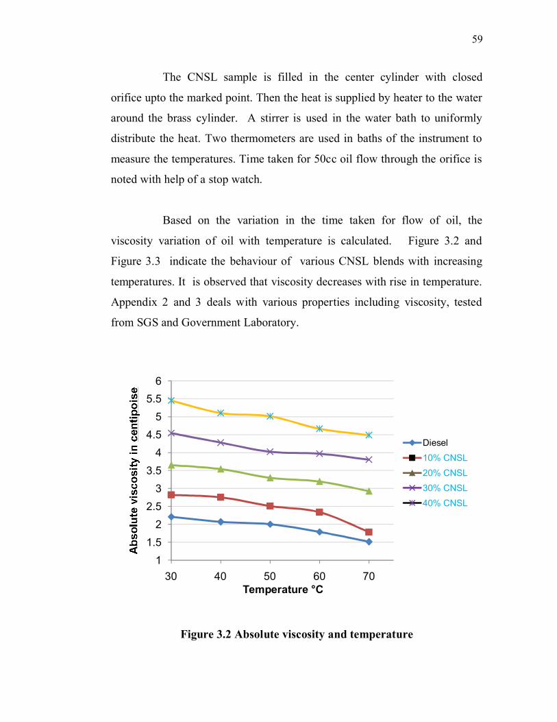
The CNSL sample is filled in the center cylinder with closed
orifice upto the marked point. Then the heat is supplied by heater to the water
around the brass cylinder. A stirrer is used in the water bath to uniformly
distribute the heat. Two thermometers are used in baths of the instrument to
measure the temperatures. Time taken for 50cc oil flow through the orifice is
noted with help of a stop watch.
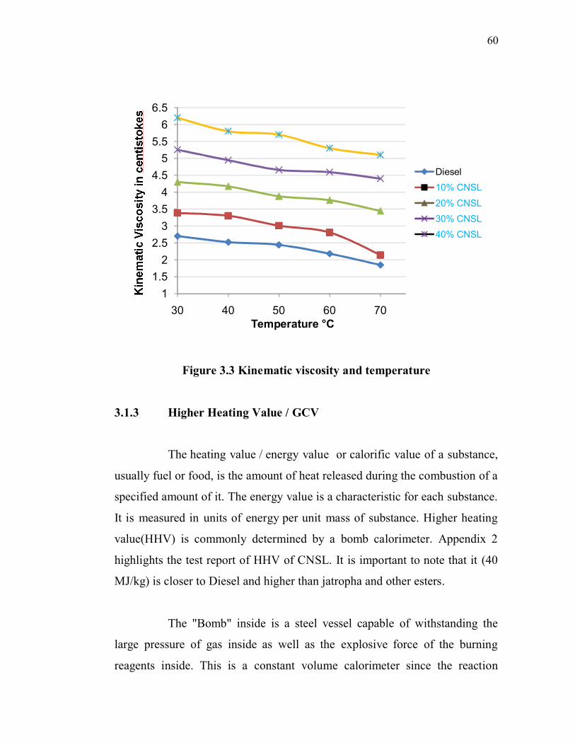
Based on the variation in the time taken for flow of oil, the
viscosity variation of oil with temperature is calculated. Figure 3.2 and
Figure 3.3 indicate the behaviour of various CNSL blends with increasing
temperatures. It is observed that viscosity decreases with rise in temperature.
Appendix 2 and 3 deals with various properties including viscosity, tested
from SGS and Government Laboratory.
Figure 3.2 Absolute viscosity and temperature
1
1.5
2
2.5
3
3.5
4
4.5
5
5.5
6
30 40 50 60 70
Temperature °C
Diesel
10% CNSL
20% CNSL
30% CNSL
40% CNSL
60
Figure 3.3 Kinematic viscosity and temperature
3.1.3 Higher Heating Value / GCV
The heating value / energy value or calorific value of a substance,
usually fuel or food, is the amount of heat released during the combustion of a
specified amount of it. The energy value is a characteristic for each substance.
It is measured in units of energy per unit mass of substance. Higher heating
value(HHV) is commonly determined by a bomb calorimeter. Appendix 2
highlights the test report of HHV of CNSL. It is important to note that it (40
MJ/kg) is closer to Diesel and higher than jatropha and other esters.
The "Bomb" inside is a steel vessel capable of withstanding the
large pressure of gas inside as well as the explosive force of the burning
reagents inside. This is a constant volume calorimeter since the reaction
1
1.5
2
2.5
3
3.5
4
4.5
5
5.5
6
6.5
30 40 50 60 70
Temperature °C
Diesel
10% CNSL
20% CNSL
30% CNSL
40% CNSL

61
occurs within a rigid vessel (the bomb) whose volume cannot change. This is
shown in the Figure 3.4.
The heat capacity of the calorimeter is equal to the sum of the heat
capacity of the water and the heat capacity of the dry calorimeter (bomb,
stirrer, insulated container, etc.) and given by the equation (3.3)
Ccalorimeter = Cdry parts + CH2O (3.3)
Figure 3.4 Bomb calorimeter
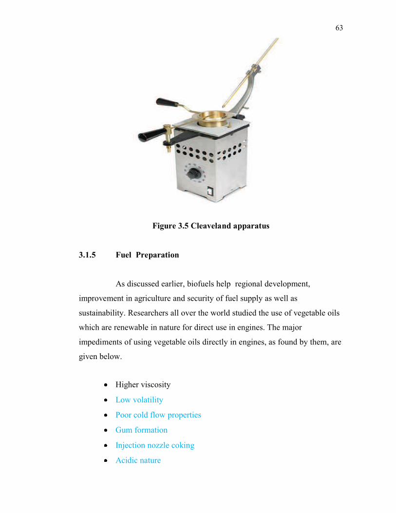
3.1.4 Fire Point and Flash Point
The Cleaveland apparatus used in the laboratory is shown in the
Figure 3.5. The test results were verified by the reports from external sources
as per Appendix 3.
The fire point was found to be 233 C and the flash point is 16
degrees below the fire point. The flash point at which CNSL starts giving
62
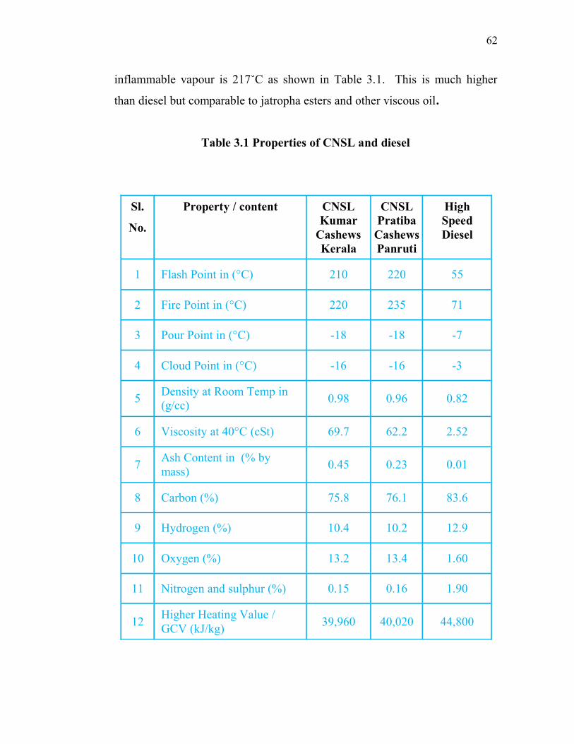
inflammable vapour is 217 C as shown in Table 3.1. This is much higher
than diesel but comparable to jatropha esters and other viscous oil.
Table 3.1 Properties of CNSL and diesel
Sl.
No.
Property / content CNSL
Kumar
Cashews
Kerala
CNSL
Pratiba
Cashews
Panruti
High
Speed
Diesel
1 Flash Point in (°C) 210 220 55
2 Fire Point in (°C) 220 235 71
3 Pour Point in (°C) -18 -18 -7
4 Cloud Point in (°C) -16 -16 -3
5Density at Room Temp in
(g/cc) 0.98 0.96 0.82
6 Viscosity at 40°C (cSt) 69.7 62.2 2.52
7Ash Content in (% by
mass) 0.45 0.23 0.01
8 Carbon (%) 75.8 76.1 83.6
9 Hydrogen (%) 10.4 10.2 12.9
10 Oxygen (%) 13.2 13.4 1.60
11 Nitrogen and sulphur (%) 0.15 0.16 1.90
12Higher Heating Value /
GCV (kJ/kg) 39,960 40,020 44,800
63
Figure 3.5 Cleaveland apparatus
3.1.5 Fuel Preparation
As discussed earlier, biofuels help regional development,
improvement in agriculture and security of fuel supply as well as
sustainability. Researchers all over the world studied the use of vegetable oils
which are renewable in nature for direct use in engines. The major
impediments of using vegetable oils directly in engines, as found by them, are
given below.
Higher viscosity
Low volatility
Poor cold flow properties
Gum formation
Injection nozzle coking
Acidic nature

64
After processing the biofuel, its property improves. Then it is
called biodiesel. Important methods of producing biodiesel, are pyrolysis -
by application of thermal energy, microemulsification which involves
surfactants for dispersions, transesterification using chemical treatment to
convert fatty acids into esters by chemical reaction and blending. Blending is
done by mixing the oil with diesel in less proportion for use in engines. CNSL
is blended with diesel, 10 to 40% by volume and tested in engines.
3.2 INVESTIGATION IN GREAVES ENGINE
In internal combustion engine, combustion of a fuel occurs with
an oxidizer as shown in Figure 3.6. Expansion of the high temperature and
high pressure gases produced by combustion applies direct force to some
component of the engine, such as pistons, blades, etc. This force moves the
component over a distance, generating useful mechanical energy.
Figure 3.6 IC engine principle
While there have been many stationary applications, the real
strength of IC engines, is in mobile applications such as automobiles, trains,
aircraft, and ships, from the smallest to the largest. Most of the IC engines use

65
4 strokes. In Suction Stroke the piston moves down from the top. As a result,
inlet valve opens (driven by gears and cam) and air is drawn into the
cylinder. After the air is drawn from the atmosphere the suction valve closes
about 30 after Bottom Dead Centre (BDC). Then Compression occurs when
the piston moves up to compress the entrapped air to induce high temperature
and high pressure enough to ignite the injected fuel just before the piston
reaches the Top Dead Centre (TDC).
Power stroke takes place (with valves closed) during the
downward stroke. Due to the combustion of fuel, hot gases at high pressure
(upto 90 bar for diesel engines) are formed. They expand adiabatically,
pushing the piston down doing useful work. In the Exhaust Stroke the inlet
valve gets closed while exhaust valve opens to allow the burnt gases to leave
the engine and thus the cycle is repeated continuously delivering power.
The fuel, which is the key-player in engine performance, must be
specially processed - usually from fossil resources for better ignition and
combustion characteristics. Biofuels must be technically and environmentally
acceptable; they must be economically competitive too in order to achieve the
desired IC engine usage. Generally biofuels from plants, can not be used
directly as engine fuels, but only in some specially modified engines. But the
engine modifications are not cheap.
As mentioned in division 3.1, neat diesel and CNSL blends are
used as fuel in compression ignition DI and IDI diesel engines. Investigations
were carried out in 3 stages and the analysis on combustion, performance and
emission are done to evaluate the impact of CNSL - Diesel blends in CI
engines. The results are evaluated with neat diesel as base.

66
The first performance test was conducted using a small air-cooled
engine, Greaves make (based on Lombardini’s design), with the main aim of
CNSL’s usage in transportation sector. When this experimental test rig was
being fabricated, just then Greaves’ light diesel engine sales volume crossed
2 million mark. In early 2012, within three years span another million
engines were sold out totaling 3 million.
The first step is to measure the calculated quantity of CNSL for
10%, 15%, 20% by volume. Then they are poured into the jar. The remaining
quantity is calculated for diesel. Corresponding amount of diesel is poured
into the respective jar and stirred manually with a glass rod for 10 minutes or
a magnetic stirrer for higher volumes and the blends are ready for testing.
3.2.1 Greaves Engine Experimental Setup
The test rig has been fabricated to comply with the loading
requirements for performance testing. The photo of the test rig in position
with the engine has been shown in Figure 3.7 and 3.8. Valve timing diagram
is shown in Figure 3.9 and performance rating in the Figure 3.10.
Performance testing rig constitutes the following equipments:
o Cylindrical tube graduated in 5ml steps
o Spring balance – 2 no’s
o Rope for loading, stopwatch and tachometer
o Setup to apply load according to the requirement
Lombardini is a pioneer in high rpm small diesel engines in the
world. The test bed was fabricated using steel sections in a rugged way to
ensure that the performance is done with less vibration. At the output pulley
shaft a rope was wrapped around to create friction for the braking torque
67
required for loading the engine. The air cooling by the fan is sufficient for the
cooling of the engine and dynamometer. This method worked satisfactorily
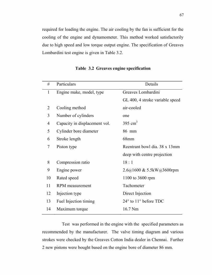
due to high speed and low torque output engine. The specification of Greaves
Lombardini test engine is given in Table 3.2.
Table 3.2 Greaves engine specification
# Particulars Details
1 Engine make, model, type Greaves Lombardini
GL 400, 4 stroke variable speed
2 Cooling method air-cooled
3 Number of cylinders one
4 Capacity in displacement vol. 395 cm3
5 Cylinder bore diameter 86 mm
6 Stroke length 68mm
7 Piston type Reentrant bowl dia. 38 x 13mm
deep with centre projection
8 Compression ratio 18 : 1
9 Engine power 2.6@1600 & 5.5kW@3600rpm
10 Rated speed 1100 to 3600 rpm
11 RPM measurement Tachometer
12 Injection type Direct Injection
13 Fuel Injection timing 24° to 11° before TDC
14 Maximum torque 16.7 Nm
Test was performed in the engine with the specified parameters as
recommended by the manufacturer. The valve timing diagram and various
strokes were checked by the Greaves Cotton India dealer in Chennai. Further
2 new pistons were bought based on the engine bore of diameter 86 mm.

68
Figure 3.7 Greaves DI engine setup
Figure 3.8 Greaves test engine drawing

69
IVO – Inlet valve open IVC – Inlet valve close F.I. – Fuel injection
EVO – Exhaust valve open EVC – Exhaust valve close
Figure 3.9 Greaves GL400 engine valve timing diagram
Figure 3.10 Greaves engine performance rating

70
3.2.2 Rope Brake Dynamometer
At the output pulley shaft a rope was wrapped around to create
friction for braking torque as required for loading the engine. For every load
variation, the spring tension is adjusted such that the braking torque is
increased to the required level. This method works satisfactorily due to forced
air cooling due to high speed fan and low torque output. 2000 rpm is chosen
by manual speed control by control cable and locking arrangement.
3.2.3 Netel Smoke Meter
Netel’s smoke meter Model NPM-SM-111B (Figure 3.7 Bottom
inset) has been designed and developed to get an accurate reading of diesel
engine smoke emissions in % opacity as in Annexure 5, according to the
specifications laid down by Ministry of Surface Transport. Its use promotes
combustion efficiency for fuel economy in diesel vehicles and stationary
diesel engines. The key features of smoke meter are given below:
Alphanumeric LCD display with back light for day/night operation.
User friendly keyboard & display interactions.
Built-in 24 column printer for hard copy of the report
Autozero facility
Easy Calibration check.
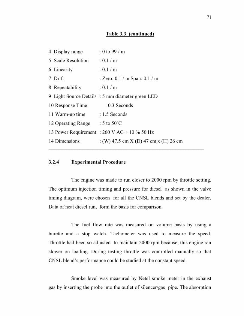
Table 3.3 Netel’s smoke meter specification
_____________________________________________________________
1 Model Number : NPM-SM-IIIIB
2 Type of smoke : Partial Flow
3 Display Indication : Light Absorption Co-efficient (K) / percentage opacity
71
Table 3.3 (continued)
4 Display range : 0 to 99 / m
5 Scale Resolution : 0.1 / m
6 Linearity : 0.1 / m
7 Drift : Zero: 0.1 / m Span: 0.1 / m
8 Repeatability : 0.1 / m
9 Light Source Details : 5 mm diameter green LED
10 Response Time : 0.3 Seconds
11 Warm-up time : 1.5 Seconds
12 Operating Range : 5 to 50ºC
13 Power Requirement : 260 V AC + 10 % 50 Hz
14 Dimensions : (W) 47.5 cm X (D) 47 cm x (H) 26 cm
____________________________________________________________
3.2.4 Experimental Procedure
The engine was made to run closer to 2000 rpm by throttle setting.
The optimum injection timing and pressure for diesel as shown in the valve
timing diagram, were chosen for all the CNSL blends and set by the dealer.
Data of neat diesel run, form the basis for comparison.
The fuel flow rate was measured on volume basis by using a
burette and a stop watch. Tachometer was used to measure the speed.
Throttle had been so adjusted to maintain 2000 rpm because, this engine ran
slower on loading. During testing throttle was controlled manually so that
CNSL blend’s performance could be studied at the constant speed.
Smoke level was measured by Netel smoke meter in the exhaust
gas by inserting the probe into the outlet of silencer/gas pipe. The absorption
72
factor in m-1
is noted down for all the performance runs. 5 sets of readings
were taken and average is used for calculation.
10% , 15% and 20% CNSL blends were used in the calibrated
burette and time taken for 5cc consumption were recorded. Flushing of the
lines using neat diesel during starting and stopping is important to avoid
denser deposit which might cause difficulty in restarting.
3.2.5 Endurance Test
There are substantial studies done by researchers to evaluate the
corrosive character of bio diesel (Sharma 2003, Avinash 2008). IS 10000 :
1980, describes the method procedure to run an endurance test on an engine at
the rated value. Change in lubricating oil property, carbon deposit on piston
and valves, cylinder head, etc. are studied after running the engine as per the
standard for 516 hours.
The test engine head was dismounted and bore was removed.
Two new pistons were weighed very accurately using Contech precision
balance (Appendix 6). Then the engine was fitted with new piston and made
to run on pure diesel for 516 hours. After the specified hours the engine was
dismounted and bore was removed. Then the engine was fitted with a new
piston and made to run in the same way for another 516 hours with 15%
CNSL blend. Then this piston was removed. Both the pistons were inspected,
measured and weighed accurately. The findings are given in Chapter 4.
New lubricating oil was changed every time when the piston got
changed. IOC lubricating oil 15W 40 was used for this test. Viscosity before
and after the tests were measured using redwood viscometer.

73
3.3 INVESTIGATION IN KIRLOSKAR IDI ENGINE
Based on the initial CNSL testing results from Greaves Cotton
engine, it was decided to proceed more technically in the Stage II
experimentation, to plot the Pressure Vs Crank Angle (P- ) graph which is a
very effective tool in testing of IC engines. The stage II investigations were
planned in a Kirloskar IDI engine - reputed for it record of extraordinary
reliability. If the CNSL graph follows the pattern of diesel, it could be better
established scientifically that CNSL would be a suitable alternative fuel in IC
engines, as per the interaction with Dr.Ganesan, IIT-M.
3.3.1 Preamble
Based on the objectives of proving CNSL as potential CI engine
fuel, it became a dire necessity to go for advanced techniques using costlier
engine testing accessories. A typical setup as described in stage III, was
offered by AVL for €41,200 with 28% additional custom duty. This worked
out to be 33 lakhs in 2010 even with the better exchange rate of 62/€. It
was also not possible to avail such testing facility outside due to the unknown
nature of CNSL. Had the emission equipment got damaged, or the engine
ceased or the pressure sensor tampered due to CNSL fuel, it would have been
a grave obscurity for the research.
Considering all the possibilities, after carefully reviewing the
unforeseen incidents happened during testing of engines using vegetable oils
in the university and IIT-M in details, it was decided to develop an affordable
state-of-the-art P- indicating system in real-time from the fundamentals,
driven by the promising potentials of CNSL and its proven sustainability.
Such an investigation called for a lot of challenges to be faced and problems

74
to be solved. Creating a cost-effective in-cylinder pressure measurement and
analysis system using innovative mechatronics approach for the first time
required different accessories and methods to be modified, evaluated and
integrated into the new measuring and indicating system. They are discussed
briefly in the proceeding sub-divisions.
3.3.2 LabVIEW Approach
Based on the earlier experience of using LabVIEW software in
thermal power stations, the author adopted a very cost-effective but reliable
approach to measure the incylinder pressure in real time with crank angle
rotation. Such a unique approach was done for the first time in engine testing,
instead of going for costlier softwares like Indimeter. To the best of the belief
of the author, the first paper in India using LavVIEW software for engine
analysis was published based on this experimentation on Kirloskar Mahabali
engine.
LABVIEW software student version 7.1- 2004, was developed by
National Instruments, USA. It can be freely downloaded and it supports all
the requirements for engine testing. It is a dataflow programming language
using graphical block diagram, but needs lot of expertise to apply. Execution
is determined by the structure of LV-source code (graphical block diagram)
on which different function-nodes are connected by drawing wires, virtually.
These wires propagate variables and any node can execute as soon as all its
input data become available. Since this might be the case for multiple nodes
simultaneously, LabVIEW is inherently capable of parallel execution. A front
panel user interface helps to start/stop, change the average of the cycles
measured and also to shift from different tasks just a mouse click. In the same
way it is possible to view the incylinder pressure measurement in a number of

75
graphical format like P- , PV or P-Q approach. If connected to a multi-
processing and multi-threading hardware it is automatically exploited to its
fullest ability by the built-in scheduler, which multiplexes multiple OS
threads over the nodes ready for execution. It has many add-on ability as
well. Due to the longevity and popularity of the LabVIEW language, and the
ability for users to extend the functionality, a large ecosystem of 3rd party
add-ons has been developed through contributions from the community. This
ecosystem is available on the LabVIEW Tools Network, and is a marketplace
for both free and paid LabVIEW add-ons.
Most of the mechatronics work done are not presented here.
However a simple description of the methodology would be helpful.
3.3.2.1 Earlier investigations
Earlier investigations used pressure sensors, charge amplifier with
oscilloscope. Edwin et al (2008) investigated rubber seed oil and inducted
hydrogen in Kirloskar engine. They computed the cylinder pressure using
signals from water-cooled Kistler sensor which is reputed for its accuracy for
decades and the position by crank angle sensor. The experiment involved
feeding the signal from the pressure sensor to the charge amplifier. A data
card integrated the optical crank angle sensor output as X-axis and pressure
signal from amplifier along Y axis. The peak pressure is obtained from the
oscilloscope output.
Purushothaman and Nagarajan (2009) completed the experimental
investigation in TAF1 engine using orange oil and orange oil with DEE using
the same methodology. Oscilloscope screenshots were printed and scaled out
manually for every 4° crank angle and pressure values were computed based
76
on the peak pressure and measured height of the screen shot. This is a very
tedious, cumbersome and laborious job. Such pressure values have to be fed
and run using a separate program in a computer. The outputs as predicted by
their program had considerable variations with the analysis of AVL’s DAS
Indimeter program output as evaluated by the author comparing them for the
same TAF1 engine. So this exquisite LabVIEW approach was developed for
P- analysis which reduced the efforts of research work extending for months
using oscilloscope method, into weeks.
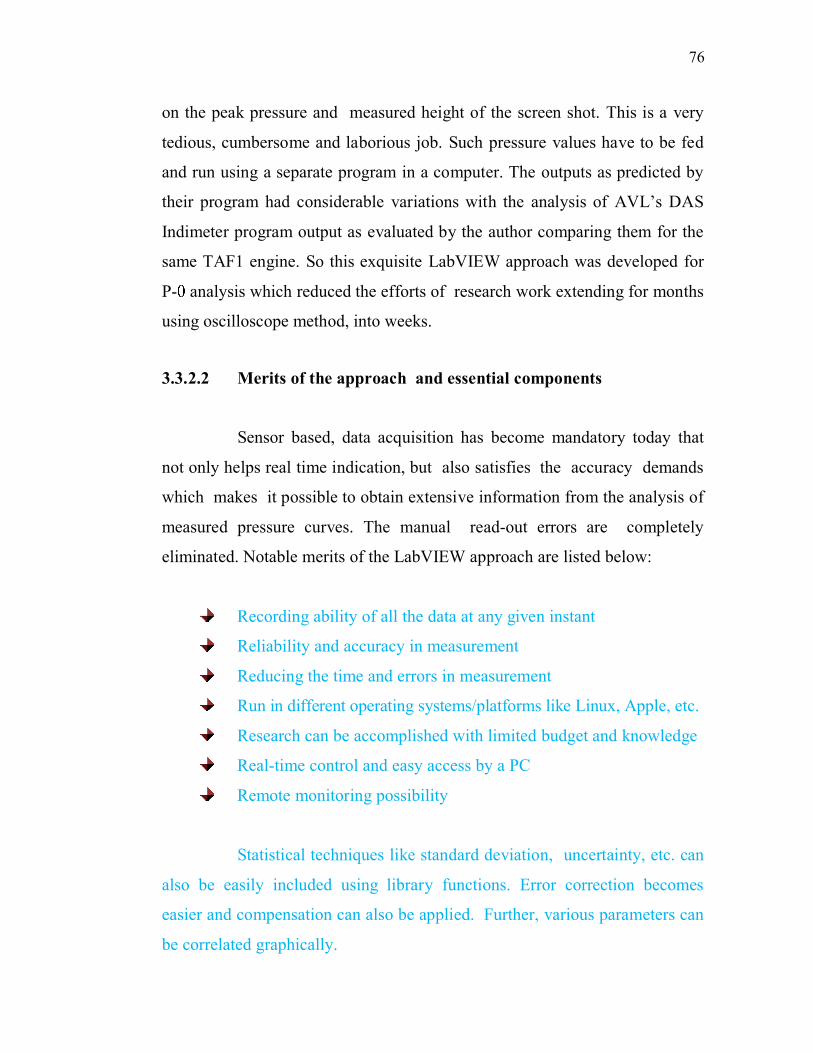
3.3.2.2 Merits of the approach and essential components
Sensor based, data acquisition has become mandatory today that
not only helps real time indication, but also satisfies the accuracy demands
which makes it possible to obtain extensive information from the analysis of
measured pressure curves. The manual read-out errors are completely
eliminated. Notable merits of the LabVIEW approach are listed below:
Recording ability of all the data at any given instant
Reliability and accuracy in measurement
Reducing the time and errors in measurement
Run in different operating systems/platforms like Linux, Apple, etc.
Research can be accomplished with limited budget and knowledge
Real-time control and easy access by a PC
Remote monitoring possibility
Statistical techniques like standard deviation, uncertainty, etc. can
also be easily included using library functions. Error correction becomes
easier and compensation can also be applied. Further, various parameters can
be correlated graphically.

77
The essential components of the data acquisition system are
sensors, signal conditioner, ADC card, LabVIEW software and computer.
The LabVIEW data acquisition system increases efficiency of measurement
and lowers the cost of testing. In power plants, using DAQ system,
engineers experience up to 10 times increase in efficiency at a fraction of the
cost - in a fraction of the time of traditional measurement system as applicable
for the same task. As mentioned before the heart of the testing arrangement is
the piezo pressure sensor and as such it was decided to use the reputed Kistler
pressure sensor 601A which is the costliest part of this testing set-up.
3.3.2.3 Test engine and modifications
Kirloskar make Mahabali 6, single cylinder IDI diesel engine as
specified in the Table 3.4, was used for this investigation with belt brake
dynamometer. Pre-combustion chamber plug was modified for the adapter of
Kistler 601A and a proximity sensor NPN type with TDC pulse facility, was
fitted to the engine body adjacent to the rotating shaft in order to measure
crank angle and thereby piston position at any given instant of time.
The Mahabali-6 (known as Indian Lister), test engine design and
construction are based on Lister, U.K. It is one of the most commonly used
stationary engine for general purpose and irrigation. It is very rugged in
construction and can be operated for long time with least maintenance.
Listeroid or Indian Lister/Lister Clones/Lister CS (cold start) are the most
versatile long running stationary engines the world had ever seen. They are
built with high factor of safety. This engine head houses the entire combustion
chamber. The CS models of engines are slow rpm (650-700rpm) 4 stroke
engines. Historically, such slow rpm IDI engines have given satisfactory
performance due to the merits of IDI and its influence on performance will be

78
discussed in Chapter 4.
The engine cylinder head, bore and pistons were dismantled and
inspected. Spare head, valves, piston and cylinder liner, gasket sets, washers
and 2 dummy plugs were bought to meet with any unforeseen damage to the
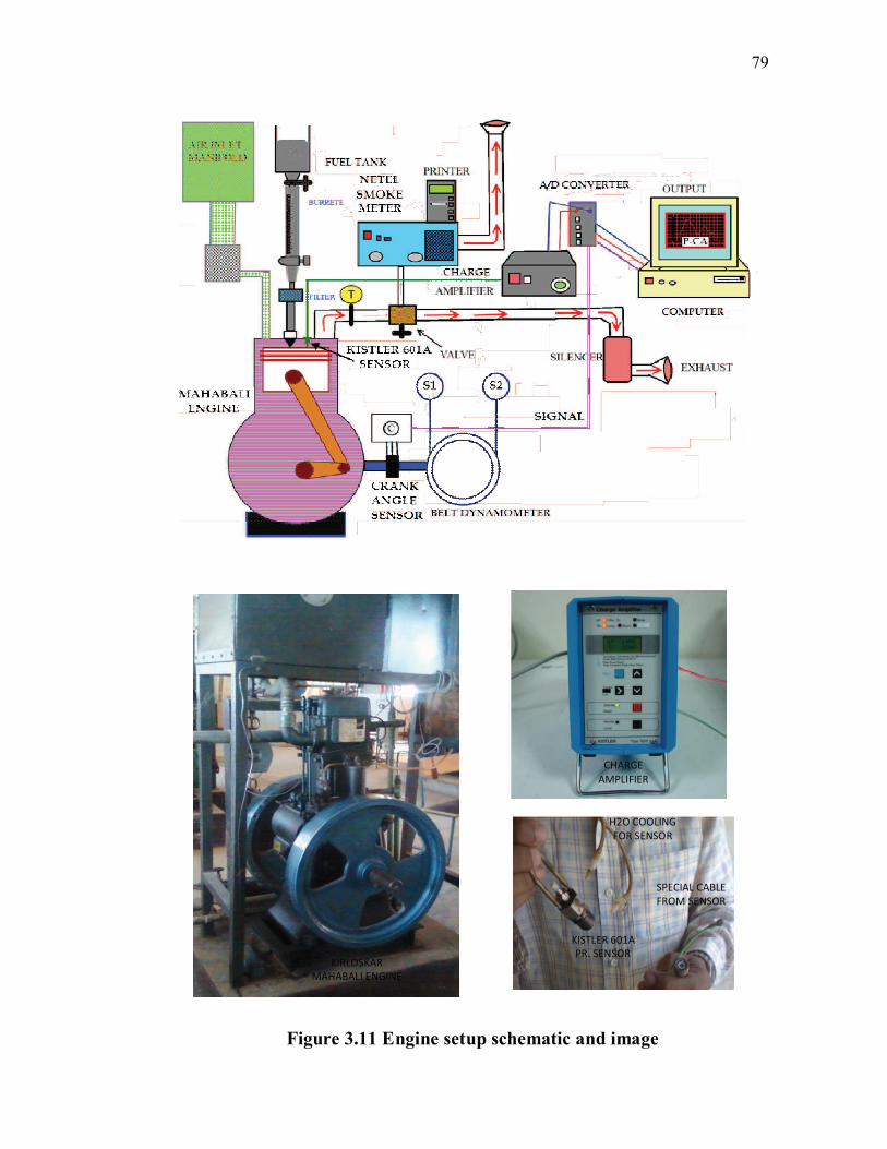
engine. The experimental setup and the schematic arrangement and photos are
shown in the Figure 3.11. The engine head has many useful functions like
housing the valves, rockers, fuel injector, water cooling passage and
connection to air inlet. The engine head is shown in Figure 3.12.
Table 3.4 Kirloskar Mahabali engine specification
# Particulars Details
1 Engine make, model, type Kirloskar Oil Engines Ltd
Mahabali 6, TRB, 4 stroke CI
2 Cooling Water cooled
3 No of cylinders 1
4 Displacement volume 1432cc
5 Cylinder bore diameter 114.3 mm
6 Stroke length 139.4 mm
7 Piston type Flat top (Lister P5050,1,2)
8 Compression ratio 17:1
9 Engine power (maximum) 4.4 kW
10 Rated speed 660 rpm, class of governing - B1
11 RPM measurement Proximity with TDC pulse
12 Fuel injection In-Direct Injection into
combustion chamber in head
79
Figure 3.11 Engine setup schematic and image
CHARGE
AMPLIFIER
KIRLOSKAR
MAHABALI ENGINE
SPECIAL CABLE
FROM SENSOR
KISTLER 601A
PR. SENSOR
H2O COOLING
FOR SENSOR

80
Name plate - front view Dummy plug hole - right side view
Injection nozzle hole - top view Valve seating - bottom view
Figure 3.12 Cylinder head parts - section and photos
1. COMBUSTION
CHAMBER
2. INJECTION NOZZLE
MOUNTING HOLE
3. DUMMY PLUG
4. METAL GASKET
5. TAPPED HOLE FOR
ADAPTER FOR PIEZO
PRESSURE
SENSOR
COMBUSTION
CHAMBER
INJECTOR
HOLE
COMB.
CHAMBER
ENTRY

81
Figure 3.13 Adapter for sensor
Figure 3.13 shows the adapter used to mount the piezo pressure
sensor (Kitler 601A). This adapter is screwed into the tapped hole at the end
of the dummy plug as indicated in Figure 3.12.
3.3.3 Brake Dynamometer
This set up consists of mechanical dynamometer with water cooled
drum. At the output shaft drum, on the right side, a belt is wrapped around it
to create friction for applying braking torque as required for loading the
engine. There are two spring balances connecting the end of the belts to the
frame. This method works satisfactorily by water cooling due to high torque at
660rpm which is maintained automatically by governor setting. There are two
spindles on the top of the spring balance to increase the loading as required.
3.3.4 Testing Procedure
Engine is loaded by increasing the tension in the belt for every
loading. 10%, 20% and 30% CNSL blends and diesel are used for every
performance run. Netel smoke meter is used to record smoke level. 5 sets of
readings for each condition are taken and recorded. LabVIEW DAS should
be run while testing for automatic collection of data to draw the P- graph.

82
3.3.5 LabVIEW Data Acquisition System
Initially LabVIEW based system was planned to capture only
pressure signal and rpm signal and merge them to plot P- diagram. But later
additional modules were integrated into a data acquisition system to display
the engine speed, exhaust gas leaving temperature and so on. This software
offers the advantage of a single point command and measurement system at a
much lower cost and featuring greater flexibility.
3.3.5.1 P- diagram significance
This pressure plotted against the crank angle is called P- diagram
which is a very useful tool for analysis. It has been long used to optimize IC
engine design and performance. The pressure inside the cylinder depends on
cylinder volume change, combustion, heat transfer to chamber walls, flow
into and out of crevice regions and leakage. Incylinder pressure is still the
central parameter that describes the in-cylinder phenomena as given below:
- The P- diagram indicates more clearly than PV diagram, the events
occurring near TDC.
- Instantaneous pressure inside the engine cylinder
- Peak pressure in the cycle and its position, mep
- Pressure rise, Position and rate of pressure rise and maximum rate
- obtain quantitative information on the progress of combustion.
- valve timing - opening and closing can be optimized.
- Rate of heat release and thus ignition delay, start of combustion, duration of
combustion and mass burned fractions, gas condition for pollutant formation
- It shows the pressure crank angle relationship for three
different rates of combustion namely high, normal and low rate.
83
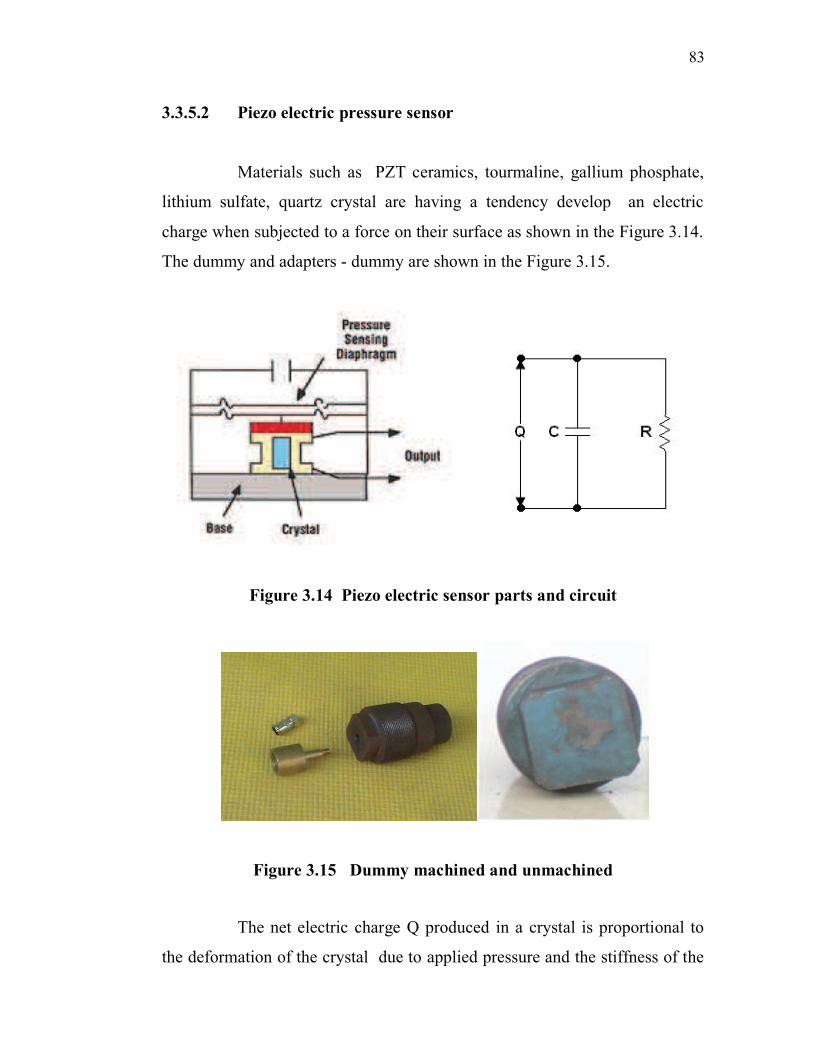
3.3.5.2 Piezo electric pressure sensor
Materials such as PZT ceramics, tourmaline, gallium phosphate,
lithium sulfate, quartz crystal are having a tendency develop an electric
charge when subjected to a force on their surface as shown in the Figure 3.14.
The dummy and adapters - dummy are shown in the Figure 3.15.
Figure 3.14 Piezo electric sensor parts and circuit
Figure 3.15 Dummy machined and unmachined
The net electric charge Q produced in a crystal is proportional to
the deformation of the crystal due to applied pressure and the stiffness of the

84
material. When a Force vector F is applied on the faces of the piezo electric
material, correspondingly a charge Q is developed between the faces as given
by equations (3.4) and (3.5) where Q is charge A is area, - stress and d11 =
piezoelectric coefficient [pC/N].
Q = A.d11. x = A.d11.F/A = d11.F (3.4)
Q = A.d12. y = I . b . d12 . F /(a . b) = d12 . F . I/a (3.5)
‘I’ is the charge and a, b are dimensions. The Governing equations
for the charge developed between faces depending upon the forces on all 6
faces and are given by the equation (3.6).
Tµ ( µ = 1 to 6) 6 faces. Tensor of the mechanical stresses (with T1 to T2 for
normal stresses x , y , z and T4 to T5 for tangential stresses yz, zx, xy.
Flow density Di = D µ . T µ (3.6)
where, Di (for I – 1to 3) is Vector of the electric flow density and
D µ is the Tensor of piezo electric coefficient accordingly in equation (3.7).
d11 d12 d13 d14 d15 d16
D µ = d21 d22 d23 d24 d25 d26 (3.7)
d31 d32 d33 d34 d35 d36 .
Finally the charge Q is calculated as given by equation ( 3.8).
Flow density Q = A . Di . ni (3.8)
Where, A is the face area and n varies from 1 to 3 components of
the normal vectors of the face.

85
Figure 3.16 Mounting of 601A sensor
The actual mounting of the piezo sensor with Water cooling
arrangement are shown in the Figure 3.16 with exploded view. Quartz sensors
can withstand very high pressure varying from 0 to 250 bar.. A hole is drilled
on the dummy plug and the pressure sensor is placed in it. The drilled hole
diameter is 5mm and an internal thread of pitch 1mm is made. The piezo
sensor is properly sealed so that there is no change in the compression ratio of
the cylinder. The pressure produced by the engine cylinder is sensed by the
pressure sensor placed on the dummy plug.
The measured pressure acts through the diaphragm on the quartz
crystal measuring element, which transforms the pressure into electrostatic
charge Q in pico coulomb. The sensor was mounted on the combustion

86
chamber plug end by M5 tapping hole to accommodate the sensor. The
complete specification of the Kistler make piezo quartz pressure sensor is
given in Table 3.5.
Table 3.5 Kistler pressure sensor specification
Particulars Details
Model and make 601 A, Kistler Instruments, Switzerland
Cooling water cooled
Range 0 to 250 bar
Overload capacity 500 bar maximum
Natural Frequency 150 kHz
Sensitivity - 14.80 pC/bar
Linearity 0.1 % FSO
Acceleration sensitivity less than 0.001 bar/g
Operating temperature -196 to 200°C
Temperature co-
efficient of sensitivity
0.0001 % /K
Shock resistance 10,000 times g ms-2
Capacitance 5 pF
Weight 1.7g
Connector, Teflon
insulator
M4 × 0.35
The stainless steel diaphragm is welded flush and hermetically to
the stainless steel body. The quartz elements are mounted in a highly sensitive
arrangement (transversal effect). It has high natural frequency. Its connector is
welded to the body, but its Teflon insulator is not absolutely tight.

87
The miniature quartz pressure sensors of the 601 Series are
especially suited for dynamic pressure measurements on objects offering
little mounting space. 601A is used in pressure measurements on combustion
engines, compressors, pneumatic and hydraulic installations (except injection
pumps). For measurements of explosion and blast pressures 601H is used.
3.3.5.3 Charge amplifier
A charge amplifier is used to convert the obtained charge into
equivalent output voltage. It just transfers the input charge to another
reference capacitor and produces an output voltage equal to the voltage across
the reference capacitor as shown by Figure 3.17. Thus the output voltage is
proportional to the charge of the reference capacitor and, respectively, to the
input charge; hence the circuit acts as a charge-to-voltage converter.
Figure 3.17 Charge amplifier circuit

88
Table 3.6 Charge amplifier specification
Particulars Details
Model and
make
5011B, Kistler Instruments
AG, Switzerland
Size and mass 70x130x170 mm ; 2kgs
Power supply 110–240 V AC @ 48 to 62 Hz
Maximum rating 0 to 999,000 pC charge input
Measuring range for 10 V full scale ±10 ... ±999 000 pC
Sensor sensitivity ±0,01 ... ±9 990 pC/bar
Scale [S] 0,001 ... 9’990‘000 bar /V
Output voltage ±10 V
Output current(short-circuit protected) ±5 mA
Output impedance 10
Frequency range
(–3dB, Filter "OFF")
0 ... 200 kHz
Low-pass filter 8 stages (1, 3, 10 ...) 0,01 ... 30 (±10) kHz (%)
Time constant [TC] (high pass filter)
Long
Medium (T = Rg Cg)
Short (T = Rg Cg)
>1 000 ... 100 000 s
1 ... 10 000 s
0.01… 100 s
Error <±100 pC FS (max./typ.) <±3/<±2%
±100 pC FS (max./typ.) <±1/<±0,5%
Linearity full scale <±0,05%
Noise mVrms <0,5 (<1,5)
9,99 pC/V (1 pC/V) mVpp <4 (<8)
Loss due to cable capacitnce <2 10– pCrms/pF
Drift at 25 °C <±0,07 pC/s
Operating temperature range 0 ... 50°C
Power, switchable VAC (%) 230/115(-22/+15)
(Protection class I) Hz (VA) 48 ... 62 (20)
Amplifier specification is depicted by Table 3.6. The input charge
Qin is applied to the summing point (inverting input) of the amplifier. It is
distributed to the cable capacitance Cc, the amplifier input capacitance Cinp
and the feedback capacitor Cf. The node equation of the input is therefore:
Qin = Qc + Qinp + Qf (3.9)
Using the electrostatic equation: Q = U.C

89
and substituting Qin, Qc, Qinp and Qf
Qin = Uinp .(Cc + Cinp) + Uf.Cf (3.10)
and solving for the output voltage Vo.
Vo = Vf = Qin/Cf which is fed into DAS. (3.11)
The output of the Kistler charge amplifier lies within ±10 V DC.
3.3.5.4 Charge Inductive Proximity Sensor
Proximity sensor detect the presence of an object nearing it. The
body style of inductive proximity sensors can be barrel, limit switch,
rectangular, slot, or ring. A barrel body style is cylindrical in shape, typically
threaded. A limit switch body style is similar in appearance to a contact limit
switch. The sensor is separated from the switching mechanism and provides a
limit of travel detection signal. A rectangular or block body style is a one
piece rectangular or block shaped sensor. A slot style body is designed to
detect the presence of a vane or tab as it passes through a sensing slot, or "U"
channel. A ring shaped body style is a "doughnut" shaped sensor, where the
object passes through center of ring. Electrical connections for proximity
sensors, inductive can be fixed cable, connector(s), and terminals. A fixed
cable is an integral part of sensor and often includes "bare" stripped leads. A
sensor with connectors has an integral connector for attaching into an existing
system. A sensor with terminals has the ability to screw or clamp down.
A small hole is drilled on the crank shaft and a pin is driven into it.
The proximity sensor is placed near it. The sensor used is of inductive type
which produces an output when a metal is placed near it. The metal is placed
at a distance of 5mm from the sensor. When the piston reaches the top dead

90
centre, the metal crosses the sensor and a TDC pulse is produced. The output
from the sensor varies from 5 to 24V. Its specification is given in Table 3.7.
Table 3.7 NPN proximity sensor specification
Particulars Details
Load Current 200 mA
Capacitive Load 1 F
Leakage Current 10 mA
Operating Voltage 10…30V DC
Voltage Drop 1V DC at 200 mA
Repeatability 10% at constant temperature
Short Circuit Protection Incorporated (trigger at 340 mA typical)
Overload Protection Incorporated
Certifications UL Listed, CSA Certified, and CE
Marked for all applicable directives
Enclosure NEMA 1, 2, 3, 3R, 4, 4X, 6, 6P, 12, 13;
IP67 (IEC529) all models;
Connections Cable: 2 m (6.5 ft) length
A2--3 -conductor PVC
C2--3 -conductor #22 AWG Tough Link
H2--3 -conductor #18 AWG Tough Link
Quick -disconnect: 4-pin mini style
4-pin micro style
LED Red: Output Energized
Inductive proximity sensors are noncontact proximity devices that
set up a radio frequency field with an oscillator and a coil. The presence of an
object alters this field and the sensor is able to detect this alteration. An
inductive proximity sensor comprises an LC oscillating circuit, a signal
evaluator, and a switching amplifier. The coil of this oscillating circuit
generates a high-frequency electromagnetic alternating field. This field is
emitted at the sensing face of the sensor. If a metallic object (switching
trigger) nears the sensing face, eddy currents are generated. The resultant
losses draw energy from the oscillating circuit and reduce the oscillations.

91
The signal evaluator behind the LC oscillating circuit converts this
information into a clear signal by effective impedance. Figure 3.18 shows its
construction and Figure 3.19 shows its operation. The sensor reduction circuit
monitors the oscillatory strength and triggers an output signal from the output
circuitry proportional to the sensed gap between probe and target.
Inductive proximity sensors are designed to operate by generating
an electromagnetic field and detecting the eddy current losses generated when
ferrous and nonferrous metal target objects enter the field. The sensor consists
of a coil on a ferrite core, an oscillator, a trigger-signal level detector and an
output circuit. As a metal object advances into the field, eddy currents are
induced in the target. The result is a loss of energy and smaller amplitude of
oscillation. The detector circuit then recognizes a specific change in amplitude
and generates a signal which will turn the solid-state output “ON” or “OFF”.
Figure 3.18 Proximity sensor parts and circuit
Figure 3.19 Proximity sensor and detection
92
The active face of an inductive proximity switch is the surface
where a high frequency electro-magnetic field emerges. A standard target is a
mild steel square, one mm thick, with side lengths equal to the diameter of the
active face or three times the nominal switching distance, whichever is
greater. For every rotation a pulse is produced and time interval also sensed.
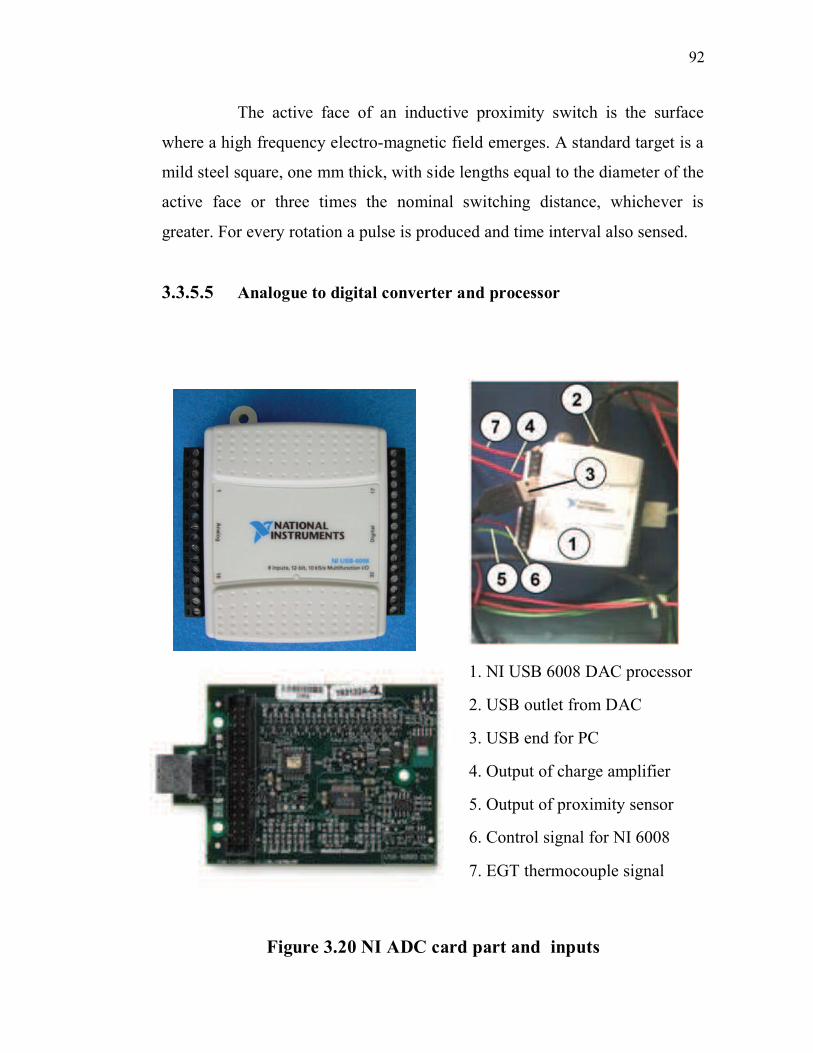
3.3.5.5 Analogue to digital converter and processor
1. NI USB 6008 DAC processor
2. USB outlet from DAC
3. USB end for PC
4. Output of charge amplifier
5. Output of proximity sensor
6. Control signal for NI 6008
7. EGT thermocouple signal
Figure 3.20 NI ADC card part and inputs
93
VI USB-6008/6009 creates a high-purity reference voltage supply
for the ADC using a multi-state regulator, amplifier, and filter circuit. The
resulting +2.5 V reference voltage can be used as a signal for self test. The
USB-6008/6009 supplies a 5 V, 200 mA output. This source can be used to
power external components. Timing resolution of 41.67 ns (24 MHz time
base) with a timing accuracy 100 ppm of actual sample rate having a
maximum 14.7 mV at 25°C noise for input analog voltage of ± 10V.
USB 2.0 full-speed with a speed of 12 Mb/s which can be directly
connected to any personal computer. The piezoelectric pressure sensor is
interfaced in the engine head and the proximity sensor is clamped at a certain
distance from the projection on the crank shaft. Figure 3.20 shows ADC card.
The analog signal from both the sensors are fed into Analog to
Digital Converter and then to the display unit through data acquisition cord
and Microcontroller. The experimental results are plotted in graph - cylinder
pressure Vs crank angle using the LabVIEW input program through control
signal wire. Investigations have been carried out for High Speed Diesel fuel
and Diesel and CNSL fuel as depicted in the graphs.
3.3.5.6 Signal evaluation and algorithms
Both pressure and proximity sensors are interfaced with the engine
and the output obtained is analog signal which is converted into digital using
ADC which is finally fed to a display unit through data acquisition cord.
Time variable, speed controlled sampling is used in this
measurement. By this measurement method, the wanted signals are sampled

94
with high resolution pulses from the crankshaft. The resulting time signal
consists of samples, that have a constant crank angle distance. The resolution
of this signal is given by the resolution of the pulse sequence. A low-pass
filtering of the signals depending on the revolution speed of the system is
necessary to avoid aliasing effects. Alternatively, from the pulse sequence of
the crankshaft a higher sampling rate for the time signal could be derived by
using a PLL-circuit. With TDC-pulse, the thus gained time signal is
synchronized to the beginning of the duty cycles and plotted over an equally
spaced abscissa. By equi-distant sampling subsequent crank angle position is
found. The signals are taken at a constant sampling rate and recorded together
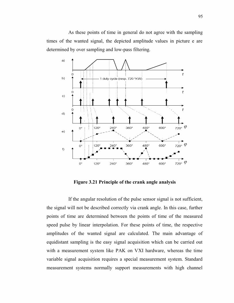
with speed and TDC pulses. The Figures 3.21 a, b and c show the acquired
signals of the measurement depicted versus time: the wanted signal, the TDC-
pulses and the speed-pulses. An engine speed pulse sensor with 3 pulses per
revolution is used. Figure 3.21 d shows the equidistant engine speed edges on
a crank angle axis. Figure 3.21 e shows the wanted signal depicted versus
crank angle. From the points of time of the engine speed edges it is
determined at which points of time amplitude values are taken from the
wanted signal.
Figure 3.21 a, b and c: wanted signal, engine speed pulses and
TDC-pulses depicted versus time.
Figure 3.21 d: speed pulses depicted versus crank angle.
Figure 3.21 e: amplitudes of the wanted signal derived at the times
of the measured speed pulses.
Figure 3.21 f: time signal versus crank angle with interpolated
speed pulses.
95
As these points of time in general do not agree with the sampling
times of the wanted signal, the depicted amplitude values in picture e are
determined by over sampling and low-pass filtering.
Figure 3.21 Principle of the crank angle analysis
If the angular resolution of the pulse sensor signal is not sufficient,
the signal will not be described correctly via crank angle. In this case, further
points of time are determined between the points of time of the measured
speed pulse by linear interpolation. For these points of time, the respective
amplitudes of the wanted signal are calculated. The main advantage of
equidistant sampling is the easy signal acquisition which can be carried out
with a measurement system like PAK on VXI hardware, whereas the time
variable signal acquisition requires a special measurement system. Standard
measurement systems normally support measurements with high channel

96
numbers which allow a simultaneous recording of many measured variables.
As the crank angle analysis of the time data is only carried out for visualizing
signals, the resolution of the crank angle axis can be varied subsequently and
other analyses of the recorded time signals are also possible. Signal extracts
can be controlled acoustically in order to investigate connections between the
acoustical perception and the signal via crank angle.
Once the pressure crank angle diagram is recorded, processing of
combustion related parameters can be done using various equations of
thermodynamic analysis. Standard algorithms built in DAS will solve the
equations fairly and accurately.
To sum up, both pressure and crank angle sensors are interfaced
with the engine through the DAS and the output obtained is analog signal
which is converted into digital using an analog to digital convertor (ADC)
which is finally fed to a display unit through Data Acquisition Cord. Real-
time measurement and control system have portability and inexpensiveness.
Computers provide high speed, mass memory, data storage and flexibility in
programming. Using data acquisition system graphical analysis, evaluating
differential equation, computing mathematical expression, display, control
and recording were done for various engine operating parameters like
instantaneous pressure, crank angle, temperature, heat release rate, PV
diagram, can be drawn using the recorded data.
For a detailed description of the basic equations required for
thermodynamic analysis which is beyond the scope of this thesis, algorithms
built in DAS solve fairly and accurately.

97
There is a wide range of calculation models, available for
thermodynamic analysis. This research work adopts double Vibe function
algorithm to approximate the actual heat release characteristics of an engine.
Consider “x” as the cumulative normalized heat released (mass fraction
burned) as given by the following relation dx = dQ/Q, where Q is the total
heat input by the fuel leading to the vibe function as given by equation (3.12).
dx
= C (m+1) . (Ø/ Øz)m . exp (-C(Ø/ Øz)m+1 (3.12)
d(Ø/ Øz)
Ø - is angle between initial and current time of the simple
Vibe function,
Øz- is the duration angle of the simple Vibe function
(duration of the heat release),
m - is Vibe function shape parameter,
C - is Vibe function parameter, C = 6.9 for complete combustion.
The integral of the Vibe function gives the fraction of the fuel mass that has
been burned since the start of combustion. Integral values are given by the
equation (3.13) and (3.14).
x = 1 - exp (-C(Ø/ Øz)m+1 and x1 = g .x, (3.13)
x1 = g .{1 - exp (-C(Ø/ Øz)m+1 }, (3.14)
where:
m1 – is the first Vibe function shape parameter,
Ø1 – is angle between initial and current time of
the first Vibe function,
Øz1 – is duration angle of the first Vibe function, and
g – is the share of fuel mass burnt as described by the first Vibe function.
98
The superposition of two Vibe (double Vibe) functions is used to
approximate the measured heat release characteristics of a diesel engine
with direct injection more accurately (Zahurul 2012). In this case, two Vibe
functions are specified, the first equation is used to model the pre-mixed
combustion and the second equation is used to model the diffusion controlled
combustion. These functions are described by equations (3.15), (3.16) and
3.17.
x2 = (1- g) . x = (1- g ){1 - exp (- C(Ø2/ Øz2)m2+1 } (3.15)
x = x1 + x2 (3.16)
dx / d = dx1/ d + dx2/ d (3.17)
where:
dx / d – is normalized rate of heat released,
– is crank angle (CA),
m2 – is the second Vibe function shape parameter,
Ø2 – is angle between initial and current time of the second
Vibe function, and
Øz2 – is duration angle of the second Vibe function (duration
of the heat release)
3.3.6 Tests with Variable Compression Ratio
IDI combustion chamber dummy plug is used to alter the clearance
volume inside the head. By inserting it deeper CR can be increased and vice
versa. Performance tests data were recorded for CR 15.5, 17 and 18.5 for
30% CNSL blend. Smoke meter readings were also noted for no load to full
load conditions and details are discussed in section 4.3.

99
3.4 INVESTIGATION IN KIRLOSKAR DI ENGINE
In the final stage III, the test engine used is Kirloskar make TAF1,
single cylinder, naturally aspirated and air-cooled with a maximum power
output of 4.4 kW. AVL’s advanced DAS, Indimeter combustion analysis
software and latest emission testing equipments have been used here.
Table 3.8 Kirloskar TAF1 engine specification
# Particulars Details
1 Engine make, model, type Kirloskar Oil Engines Ltd
TAF 1, 4 stroke CI engine
2 Cooling air-cooled
3 Number of cylinders one
4 Displacement volume 661.5 cm3
5 Cylinder bore diameter 87.5 mm
6 Stroke length 110 mm
7 Piston type Hemi spherical bowl at centre
8 Compression ratio 17.5 : 1
9 Engine power (maximum) 4.4 kW
10 Rated speed 1500 rpm
11 RPM measurement Proximity with TDC pulse
12 Fuel injection Direct
13 Fuel injection timing 24° before TDC
14 Injection pressure 210 bar
100
3.4.1 Test Engine
Kirloskar TAF1 is one of the most widely used engines in India,
especially for agriculture. It is rugged in construction and can run unattended
for days. Since it is air-cooled, it can be used at any place where water
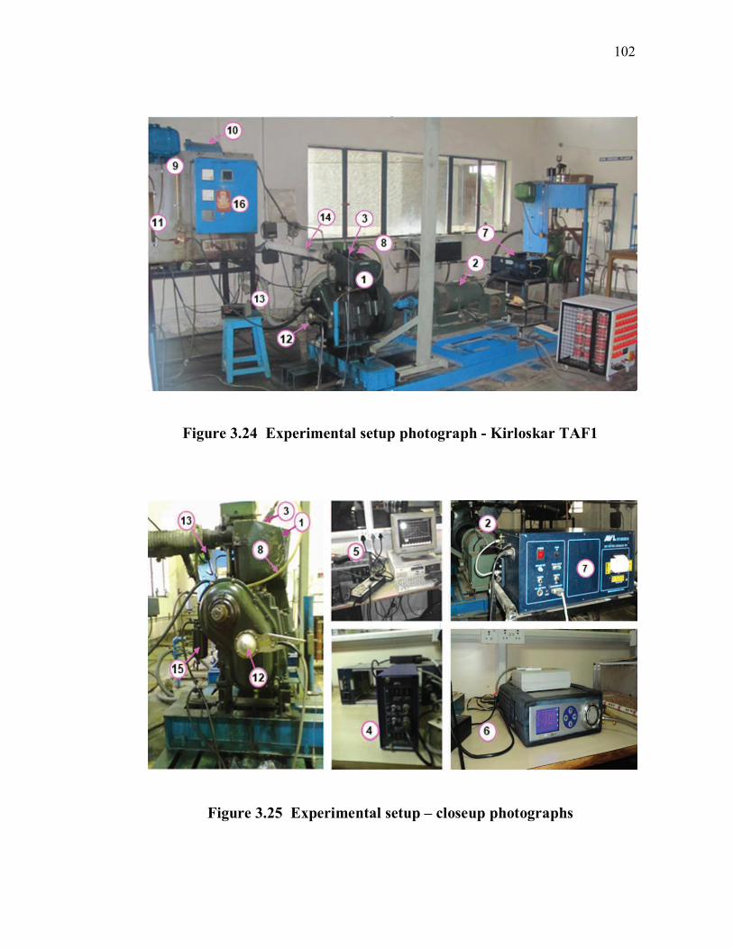
connection is not available/possible. The engine specification is given in the
Table 3.8. The complete experimental setup, general arrangement of the
equipments and components of the testing system are shown schematically in
Figure 3.23 and photographically in Figure 3.24 and Figure 3.25.
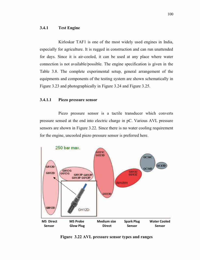
3.4.1.1 Piezo pressure sensor
Piezo pressure sensor is a tactile transducer which converts
pressure sensed at the end into electric charge in pC. Various AVL pressure
sensors are shown in Figure 3.22. Since there is no water cooling requirement
for the engine, uncooled piezo pressure sensor is preferred here.
Figure 3.22 AVL pressure sensor types and ranges
M5 Direct M5 Probe Medium size Spark Plug Water Cooled
Sensor Glow Plug Direct Sensor Sensor

101
Figure 3.23 Experimental setup diagram - Kirloskar TAF1
1. Test engine 2. Electrical dynamometer
3. Pressure sensor 4. Charge amplifier
5. Data acquisition system 6. Flue gas analyzer DiGAS 444
7. Smoke meter AVL 437C 8. Fuel injection nozzle and hose
9. Diesel tank with burette 10. Biofuel tank with burette
11. Manometer and orifice 12. Crank angle sensor AVL 364
13. Exhaust pipe thermocouple 14. Exhaust gas to silencer
15. Fuel filter 16. Voltage - Current - rpm panel
102
Figure 3.24 Experimental setup photograph - Kirloskar TAF1
Figure 3.25 Experimental setup – closeup photographs

103
AVL piezo pressure sensor model GH12D is chosen for testing,
because it is highly accurate, front-sealed, cylindrical and gives better
performance in heavy duty applications for compression ignition engines.
Table 3.9 gives the salient details about this sensor.
Table 3.9 AVL pressure sensor GH12D specification
Details Value
Measuring range 250 bar
Piezo material Gallium Phosphate – GaPO4
Sensitivity 16 pC/ bar
Linearity ±0.3% FSO
Acceleration
Sensitivity
< 0.001 bar/g axial
– 0.0003 bar/g radial
Shock resistance > 2000 g
Temperature range -40°C to +400°C
Thermal sensitivity shift 20…400°C < 2%, 200…300°C < 0.5%
Cyclic temperature drift < ±0.5 bar (@ 1300 rpm / 7 bar IMEP)
Max. load change drift grad. 1.0 mbar/ms
Mounting torque 1.5 Nm
The transducer is mounted on the engine by M5 thread via an
adaptor sleeve screwed onto the engine head. A special low impedance cable
connects the sensor output into a charge amplifier. Due to GaPO4 crystal
measuring element, this set is ideally suited for high precision pressure
measurements under limited space though it is many times costlier than
Quartz sensor which needs water cooling as discussed in sub-division 3.3. For
104
signal processing a free input channel with charge amplifier must be
available for the indicating system.
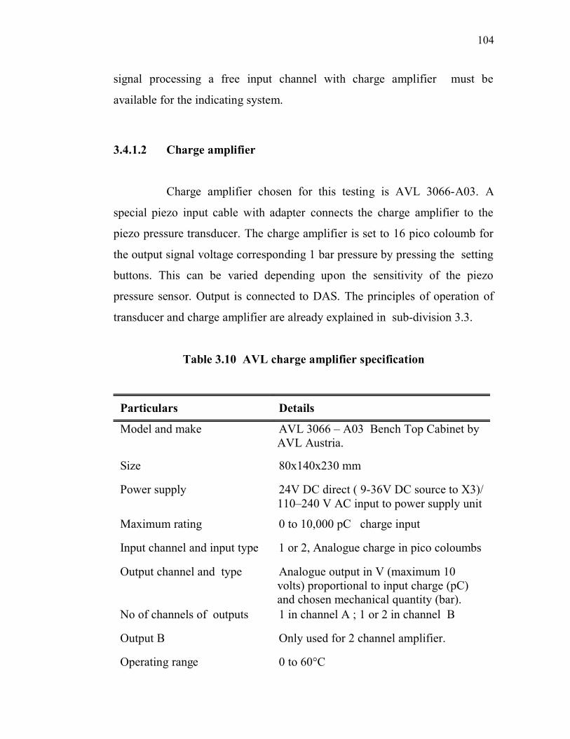
3.4.1.2 Charge amplifier
Charge amplifier chosen for this testing is AVL 3066-A03. A
special piezo input cable with adapter connects the charge amplifier to the
piezo pressure transducer. The charge amplifier is set to 16 pico coloumb for
the output signal voltage corresponding 1 bar pressure by pressing the setting
buttons. This can be varied depending upon the sensitivity of the piezo
pressure sensor. Output is connected to DAS. The principles of operation of
transducer and charge amplifier are already explained in sub-division 3.3.
Table 3.10 AVL charge amplifier specification
Particulars Details
Model and make AVL 3066 – A03 Bench Top Cabinet by
AVL Austria.
Size 80x140x230 mm
Power supply 24V DC direct ( 9-36V DC source to X3)/
110–240 V AC input to power supply unit
Maximum rating 0 to 10,000 pC charge input
Input channel and input type 1 or 2, Analogue charge in pico coloumbs
Output channel and type Analogue output in V (maximum 10
volts) proportional to input charge (pC)
and chosen mechanical quantity (bar).
No of channels of outputs 1 in channel A ; 1 or 2 in channel B
Output B Only used for 2 channel amplifier.
Operating range 0 to 60°C

105
Table 3.10 (continued)
Transducer sensitivity 0.1 to 99.9 pC ±0.5
Output selection range 20 bar / V gives a maximum pr. 100bar
Input pressure range
(depends on piezo sensor)
Upto 500 bar with sensor sensitivity of 20
pC/bar; upto 1250 bar for sensitivity of 8.
Hum and noise Less than 1 mV RMS or 10mV peak to
peak (0 to 50 MHz)
Linearity error less than 0.01% of FSO
Low-pass filter 2,5,10,20,50 or 100 kHz upper cut-off
Gain resolution 8 bit
Averaging upto 100 cycles or cycle-by cycle value
Drift compensation continuous or cyclic by self precise self
voltage generation.
3.4.1.3 Crank angle optical encoder
For accurate measurement of the crank position at any instant of
time, AVL 364 encoder is used. This Crank Angle Encoder is a high precision
optical sensor with respect to angle-related measurements, mainly for
indicating purposes. It is mounted on the free end of the crank shaft as shown
in the Figure 3.27. The necessary power is supplied by an AC to DC converter
with an output of 15V± 4%.
The optical function is based on a slot integrated marker disk and
utilises the light reflection principle. It is the most common method used in
engine indicating technology due to its stability in extreme operating
conditions. The angle mark resolution is 0.5 degree crank angle (up to 0.1°
CA by means of multiplication called dynamic accuracy). A fibre optic cable

106
carries the light pulse signal to the mounted emitter-receiver electronics at the
other end. The electronic components are located separately from the sensor,
in order to minimise the influence of electric interference, temperature and
vibration. There is one track on the marker disk with 720 pulses for the angle
information which includes trigger pulse information per revolution meant
for synchronisation purposes. This is also used for locating TDC timing in the
CA signals.
The opto-electronic converter, converts the light signal into digital
signal pulse which is used as an input to the Data Acquisition Card (DAC)
using signal conditioning interface. The pressure sensor and position sensor
locations are shown in the photograph of the experimental setup. The crank
angle sensor AVL 364 optical encoder is shown in Figure 3.26.
Figure 3.26 Crank angle encoder drawing

107
Figure 3.27 AVL 364 optical sensor photograph
To sum up, light rays are cut by the precision slots of the rotating
disc mounted at the end of the engine shaft. This can measure the angular
position to an accuracy of 0.5°. It has to be rigidly mounted as shown in the
setup arrangement and its only disadvantage is that it needs an open crank
shaft end for mounting. Its salient merits are given below:
High precision and resolution
Compact size with low-mass and therefore low inertia
High tensile strength materials (titanium shaft, high tensile housing)
High mechanical resistance, several hundred of g
Working temperature range of 400 to 700 °C (electronics) and
mechanical parts upto 1200°C
Precise measurement upto a speed of 20,000 rpm
Rotary and torsional analysis are possible
Selectable output pulses per revolution 36, 720, ….1800, 3600
Second output 36 to 720 pulses/sec.
Application can be stationary engine or moving automobile engine
Usage - small bike engines to large ship engines
Cost saving version in combination with AVL Indimeter software

108
3.4.1.4 DAC and indicating software
The experimental investigation adopts AVL’s proprietary Data
Acquistion Card (DAC) and DAS software - Indimeter 617 version 2.0 which
is based on the good-old, proven MS-DOS operating system. There is an
analog to digital converter which converts the charge amplifier output of
incylinder pressure signal and also other analogue signals. It can also take
digital input signals and process them.
AVL’s Indimeter 617 is reputed for it’s smaller software file
size and combination of signal amplification with powerful data acquisition
for a wide range of automobile applications. Four analog inputs and two
digital inputs for preconditioned and multiplexed current clamp signals,
enable recording of all the necessary information, which is synchronized
with the AVL 364 crank angle encoder signal with TDC pulse. An integrated
RS232 interface supports the real time raw data transfer to a personal
computer. The operating system of the PC is Windows 98. It can also be
operated in stand alone mode providing the facility of real-time processed
results’ values for post data processing while the engine and all signals are
OFF.
Indimeter 617 is a versatile software for real-time data acquisition,
post processing, graphical presentation, documentation and exporting data
to flash drive/CD writer. Further, crank angle based data acquisition, with
simultaneous real-time evaluation of indicating results, enables plotting of P-
and P-V diagram. It also has provisions for oscilloscope mode with single
measurement in real-time and multi-channel digital voltmeter as well. There
is a also a recorder for time based measurement and integration into ECU

109
calibration software with digital signal filtering. Misfire detection based on
monitoring of indicated mean effective pressure is also possible.
Indimeter 617 offers extensive possibilities for selection,
organising, presentation and correlation of any kind of measuring data as well
as for report generation using Microsoft Excel package. The unlimited direct
access to recorded data, indicating data or measuring point files, helps easy
comparison of different data sets. Indimeter’s salient features are given
below:
Power supply 9 to 36 V DC
Power consumption 25 W
Operating temperature range -35°C to 50°C
ADC resolution 16 Bit
Fast and easy set-up due to crank angle auto diagnostics and
reliability by utilizing real time plausibility checks
Analog input signal +/- 10V
4 analog voltage input channels and 2 digital input channels
Sampling rate per channel 1MHz per channel
Digital channels used for multiplexed ignition or injection signals,
measured via current clamp and AVL Pulse
Linearity +/- 0.01% FS
Data and graphic export via ASCII files
Data post processing facility
Low-pass filter free-definable cut-off frequency between
5-100 kHz
Drift compensation cyclic or continuous drift compensation modes
Wide selection of presentation possibilities: line, bar, x-y graphs,
tables, etc.
110
3.4.1.5 Precautions
For best signal quality the following precautions are followed:
The amplifier input cable is kept short.
The amplifier input cable is installed as far away from other cables
as possible.
Signal cables should not be subjected to high mechanical stress.
The connections of the input cable are kept clean and dry.
Signal cables should not be conduited with power cables.
Twisting of cables is to be avoided.
No sharp bend, hard object hitting on the cable
3.4.2 Electrical Dynamometer
Powerstar electrical dynamometer is made by Mantra Engineering
Manufacturing Limited, Coimbatore. It is coupled with the test engine crank
shaft on the rightside. Crank angle encoder AVL 364 is connected to the
leftside of crank shaft open end, as discussed earlier. Its model is 21-9
having a maximum rating of 5kW with the highest current rating of 21A.
Electrical resistance loading is used to load the engine from 0%, 25%, 50%
and 100% representing 1.1kW, 2.2kW, 3.3kW and 4.4kW respectively.
Loading can be easily done by switching on the required
resistance bank according to the testing requirements. The alternator is 4
pole, single phase, 50 Hz, 240V output with a capacity of 5 kVA working
under the principle of Faraday’s electromagnetic induction. If the rpm is
lower than 1500, correspondingly the frequency will get reduced
proportionately. However the voltage is not affected due to its flat
characteristic curve. At any loading, current in any of the branches should not
111
exceed 21A which is the rating of winding wires. The voltage, current and
rpm readings are measured in the load panel for calculating the engine power.
3.4.3 Emission Equipment
The most important feature of the experimental setup is the
emission measuring arrangement. AVL smokemeter 437C is kept closer to
the exhaust line whereas the AVL DiGAS 444 five gas analyser (O2, CO2,
CO, HC and NOx) is kept near DAS and PC.
.
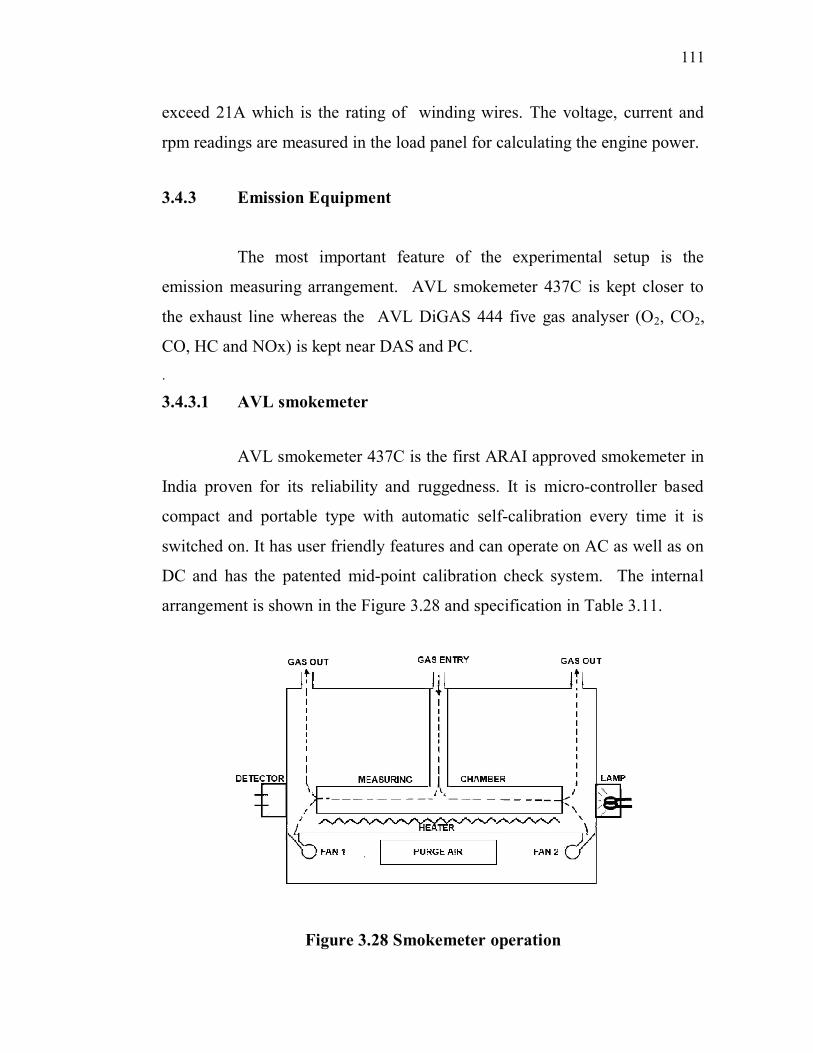
3.4.3.1 AVL smokemeter
AVL smokemeter 437C is the first ARAI approved smokemeter in
India proven for its reliability and ruggedness. It is micro-controller based
compact and portable type with automatic self-calibration every time it is
switched on. It has user friendly features and can operate on AC as well as on
DC and has the patented mid-point calibration check system. The internal
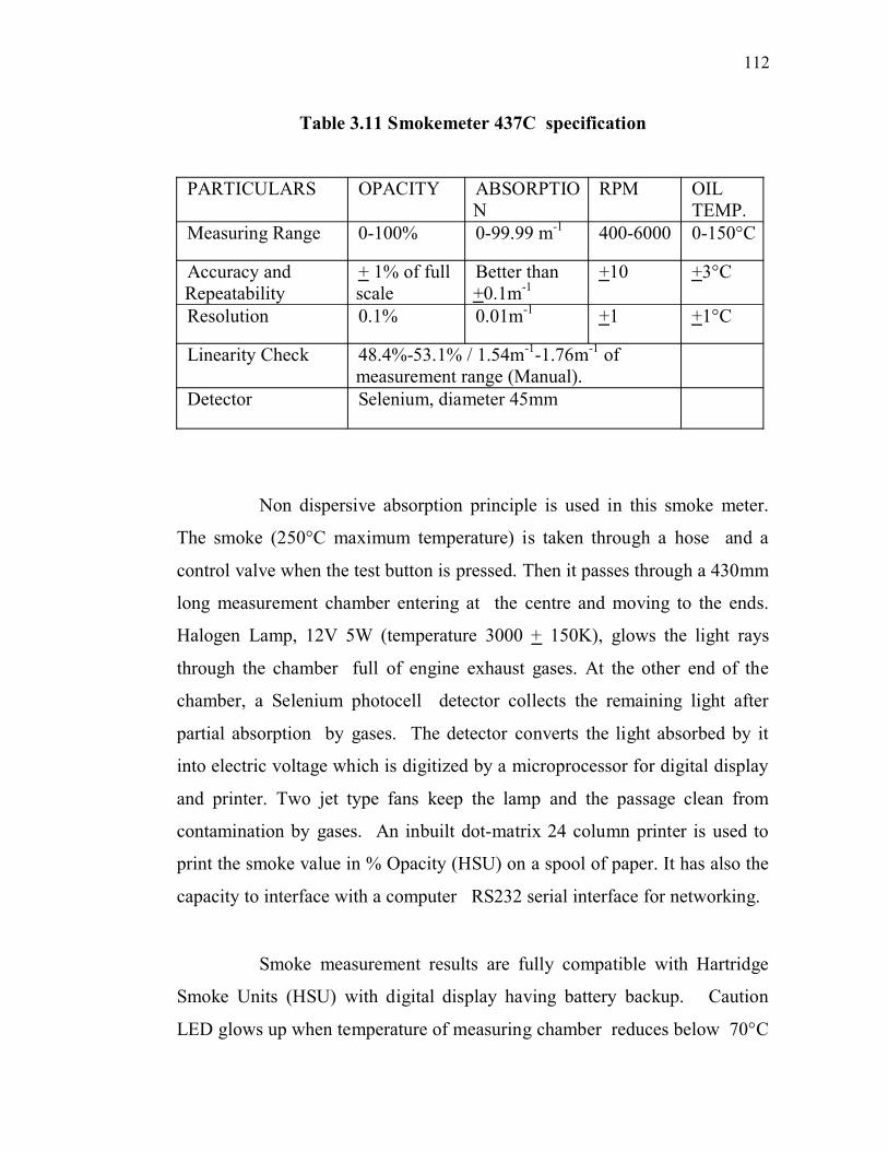
arrangement is shown in the Figure 3.28 and specification in Table 3.11.
Figure 3.28 Smokemeter operation
112
Table 3.11 Smokemeter 437C specification
PARTICULARS OPACITY ABSORPTIO
N
RPM OIL
TEMP.
Measuring Range 0-100% 0-99.99 m-1
400-6000 0-150°C
Accuracy and
Repeatability
+ 1% of full
scale
Better than
+0.1m-1
+10 +3°C
Resolution 0.1% 0.01m-1
+1 +1°C
Linearity Check 48.4%-53.1% / 1.54m-1
-1.76m-1
of
measurement range (Manual).
Detector Selenium, diameter 45mm
Non dispersive absorption principle is used in this smoke meter.
The smoke (250°C maximum temperature) is taken through a hose and a
control valve when the test button is pressed. Then it passes through a 430mm
long measurement chamber entering at the centre and moving to the ends.
Halogen Lamp, 12V 5W (temperature 3000 + 150K), glows the light rays
through the chamber full of engine exhaust gases. At the other end of the
chamber, a Selenium photocell detector collects the remaining light after
partial absorption by gases. The detector converts the light absorbed by it
into electric voltage which is digitized by a microprocessor for digital display
and printer. Two jet type fans keep the lamp and the passage clean from
contamination by gases. An inbuilt dot-matrix 24 column printer is used to
print the smoke value in % Opacity (HSU) on a spool of paper. It has also the
capacity to interface with a computer RS232 serial interface for networking.
Smoke measurement results are fully compatible with Hartridge
Smoke Units (HSU) with digital display having battery backup. Caution
LED glows up when temperature of measuring chamber reduces below 70°C

113
or voltage is low. The chamber is electrically heated by thermostatically
controlled rheostat to 100 ±5°C so as to avoid condensation of moisture and
measurement errors. It also indicates the error message if there is any deposit
on the bulb or photocell after a long usage.
3.4.3.2 AVL DiGAS 444 gas analyser
The 5 gas analyser used is AVL make DiGAS 444 which is a very
accurate and fast responding analyser as specified in the Table 3.12. Flue gas
from the exhaust pipe tapping is taken through a rubber hose to the analyser.
Table 3.12 DiGAS analyser specification
Particulars /
method
Measuring
time
Resolutio
n
Accuracy
CO / NDIR 0…10 % vol. 0.01 %
vol.
<0.6 % vol: + 0.03 % vol.
>0.6 % vol: + 5 % of
Indicated value
CO2 / NDIR 0…20 % vol. 0.1 % vol. <10 % vol: + 0.05 % vol.
>10 % vol: + 5 % of vol.
HC / NDIR 0…20000 ppm
vol.
<2000:1
ppm vol,
>2000:10
ppm vol
<200 ppm vol: + 10 ppm vol.
>200 ppm vol: + 5 %
Indicated value
O2 / NDIR 0…22% vol. 0.01 % vol <2 % vol: + 0.1 % vol.
>2 % vol: + 5 % of ind. val.
NOx / NDIR 0…5000 ppm
vol.
1 ppm vol <500 ppm vol: + 50 ppm
vol.
>500 ppm vol: + 10 % of
Indicated value
Engine Speed 400…6000
rpm
1 rpm +1 % of ind. value
Oil temp. -30… 125°C 1°C + 4°C
Lambda 0… 9.999 0.001 used for calculation of CO,
CO2, HC, O2

114
Table 3.12 (Continued)
Power supply 11 …. 22 V Dc
Warm up Time: 7 min
Calibration gas data 60…140 litres/h, max. overpressure 450 hPa
Voltage: 11…22 V DC
Power Consumption: 25 W
Connector cooling gas 180 litres/h, max. overpressure 450 hPa
Response time: t95 < 15 s
Operating
temperature:
5…45°C
Storage temperature: 0…50°C
Relative humidity: <95 %, non-condensing
Inclination: 0…90°
Dimension
(W D H)
270 320 85 mm3
Weight: 4.5 kg net weight with accessories
Interfaces: RS232 C, 24 column dot matrix printer
with LCD display
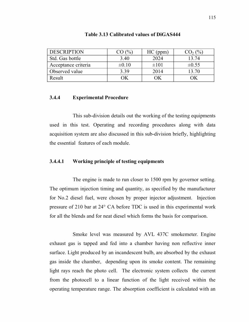
Engine exhaust emissions of unburned HC, CO2, CO, O2 and NOx
were measured on the dry basis after removing moisture. In AVL DiGas 444
flue gas analyser, Non Dispersive Infrared methodology is used. The samples
to be evaluated are passed through an inbuilt cold trap (moisture separator)
and also through the filter element to prevent water vapour and particulates
from entering into the analyzer. NOx and HC (in hexane equivalents) were
measured in parts per million (ppm) and carbon monoxide, oxygen and
carbon dioxide emissions were measured in terms of percentage volume. As
per the recommendations of the supplier, the analyzer is periodically
calibrated. Calibration details of the DiGAS 444 analyser before this
experimentation are given in Table 3.13. Atmospheric O2 % and exhaust gas
O2 are measured for calculation of other gas composition using their molar
volume fractions in the engine exhaust gas.
115
Table 3.13 Calibrated values of DiGAS444
DESCRIPTION CO (%) HC (ppm) CO2 (%)
Std. Gas bottle 3.40 2024 13.74
Acceptance criteria ±0.10 ±101 ±0.55
Observed value 3.39 2014 13.70
Result OK OK OK
3.4.4 Experimental Procedure
This sub-division details out the working of the testing equipments
used in this test. Operating and recording procedures along with data
acquisition system are also discussed in this sub-division briefly, highlighting
the essential features of each module.
3.4.4.1 Working principle of testing equipments
The engine is made to run closer to 1500 rpm by governor setting.
The optimum injection timing and quantity, as specified by the manufacturer
for No.2 diesel fuel, were chosen by proper injector adjustment. Injection
pressure of 210 bar at 24° CA before TDC is used in this experimental work
for all the blends and for neat diesel which forms the basis for comparison.
Smoke level was measured by AVL 437C smokemeter. Engine
exhaust gas is tapped and fed into a chamber having non reflective inner
surface. Light produced by an incandescent bulb, are absorbed by the exhaust
gas inside the chamber, depending upon its smoke content. The remaining
light rays reach the photo cell. The electronic system collects the current
from the photocell to a linear function of the light received within the
operating temperature range. The absorption coefficient is calculated with an
116
accuracy of 0.025 m-1
. The equipment has a stored microprocessor program
as per ECE-R24 ISO 3173, so as to collect values such as exhaust gas
pressure, temperature, opacity and absorption.
Exhaust emissions of unburned HC, CO2, CO, O2 and NOx were
measured on the dry basis. In AVL DiGas 444 flue gas analyser, Non
Dispersive Infrared methodology is used. NOx and HC were measured in
parts per million and carbon monoxide, oxygen and carbon dioxide
emissions were measured in terms of percentage volume.
AVL’s software Indimeter 617 version 2.0 is used to measure the
heat release rate, inside cylinder pressure, mean effective pressure, etc. It has
got inbuilt analog to digital convertor, to convert analog signals for PC
interface. This setup uses AVL uncooled peizo transducer to measure
instantaneous combustion chamber pressure during the entire operation which
converts the pressure into charge. This charge is supplied to a charge
amplifier which amplifies the same into an equivalent voltage. The inbuilt A-
D converter has external and internal trigging facility for different channels.
Data for 50 consecutive cycles are recorded and the average value of 50
cycles is taken for generating the curves on the computer screen.
The fuel flow rate is measured on volume basis using a burette and
a stop watch. Thermocouple and a digital indicator were used to note the
exhaust gas temperature.
3.4.4.2 General operating and recording procedure
i. Calculated volume of 10%, 20%, 30% and 40% CNSL were taken in
measuring jar and mixed with 90%, 80%, 70%, 60% neat diesel
117
respectively. After using magnetic stirrer for 15 minutes blends were
ready on volume basis.
ii. Engine was allowed to run for 15 minutes to enable warming up of
components to reach stable condition for testing.
iii. Loading was done for neat diesel in 4 steps starting from 0 kW to 1.1
kW, 2.2 kW and 3.3 kW until the full load of 4.4 kW. Once the stable
running was achieved, time taken for 10cc was noted down by a
stopwatch. The voltage and current readings were taken from the
panel for calculating brake power directly. Engine speed was also
recorded for complete range of loading.
iv. Flexible hose from the flue gas tapping was taken out and connected to
the DiGas 444 analyser to record the steady value which was printed
locally. Then the hose was taken out and connected to the smokemeter
437C for recording the smoke value and the printout was taken.
v. Data acquisition system commands were used to record the 50 cycle
average for each condition of loading for every fuel blend and separate
filename was given for each loading values.
vi. Five sets of readings were recorded for each fuel composition and
average value was calculated and used for calculation in order to
reduce the experimental errors.
vii. Readings observed for standard diesel fuel are taken as the base .
viii. Subsequently four CNSL blends ranging from 10% to 40% by
volume and diesel 90% to 60% respectively, were tested one after the
other by filling the blend in the biodiesel tank. The 3way cocks were
opened and closed suitably to changeover from one blend to another.
ix. Sufficient time was allowed to empty the previous blend in the filter,
pipeline and injector lines. Warming up time of 10 minutes for each
blend is necessary to obtain accurate reading in order to assess the
118
correct behavior of each blend. Necessary modification is done as
required for the new study.
x. All the readings are recorded in the same way as described from steps
one to nine. For each blend and each loading average value of 5
measurements of each parameter is recorded in the tabular format.
xi. After completing all the testing of the blends, once again the neat
diesel was used to purge the lines containing the biofuel so that
accumulation, settling could be avoided.
xii. Fuel nozzle coking, detonation characteristics, etc. were to be carefully
observed and recorded.
Based on the stable performance of the first investigation in TAF1
engine, 30% CNSL with 70% diesel by volume is taken as the reference fuel
for all the investigations with varying parameters as enunciated in the
following sub-divisions.
3.4.5 Tests with Varied Fuel Injection Pressure
Tests were performed at the rated speed of 1500 rpm. The fuel
injection pressure was set to 195 bar, 225 bar and 240 bar. Injection pressure
was changed by means of adjusting the injector spring tension. In this
experimentation fuel injection timing is not changed. Experimental procedure
was repeated as mentioned earlier.
3.4.6 Tests with Varied Fuel Injection Timing
To study the effect of the injection timing on the combustion,
performance and emission, tests were conducted by modifying fuel injection
timing. The fuel injection timing was set to 21° before TDC and 27° before

119
TDC by means of addition and removal of standard shims respectively as
specified by the manufacturer. The shims are to be fitted between the pump
flange and the steel plate. Addition of one standard shim retards the injection
timing by 3°. Removing shim (reducing the total thickness of the shim) will
advance the injection timing. Fuel injection pressure was kept at standard
value of 210 bar and the experimental procedure was repeated for every
setting. Performance parameters and emission values were recorded.
3.4.7 Tests with Varied Inlet Valve Timing
By changing the inlet valve opening and closing timing, the
residual quantity of exhaust gas trapped inside the cylinder can be varied
which creates an effect of internal exhaust gas recirculation to reduce NOx
emission in CI engines. NOx levels of CNSL blends were always found to be
higher than that of diesel. So, Miller cycle concepts have been taken up in this
test, by altering the inlet valve timing as shown in the Figure 3.29.
Figure 3.29 New IV timings Figure 3.30 Valve tappet feeler gauge
120
The manufacturer’s set values for IVO is 4.5° before TDC and IVC
at 35.5° after BDC. The tappet clearance at cold condition is 0.18mm for
inlet valve. This clearance was increased to obtain retarded inlet valve
opening and earlier closing, inline with Miller’s concept of closing the inlet
valve at different positions w.r.t. BDC. Valve opening and closing timing is
adjusted by using a valve tappet feeler gauge shown in the Figure 3.30.
Two valve timings were chosen for this study. By increasing the
tappet clearance the inlet valve opens late and closes early as illustrated by
Figure 3.15 as follows:
a) 3 degrees (viz. IVO at 1.5° before TDC ; IVC 32.5° after BDC)
b) 6 degrees (viz. IVO at 1.5° after TDC ; IVC 29.5° after BDC)
The exhaust valve was not disturbed in this study. It opens 35.5
BTDC and closes 4.5 after TDC. Only the inlet valve timing was analysed
since it does not affect the output of the engine to that extent as Exhaust
valve. Experiments were performed using the new setting for 30% CNSL and
data are recorded.
3.4.8 Tests with Higher Fuel Inlet Temperature
Fuel inlet temperature has a very important influence on the
combustion and emission of a CI engine. The Kinematic viscosity of CNSL is
significantly higher than mineral diesel, however heating CNSL to
about 100ºC would probably resolve the problem of high viscosity and bring
the viscosity levels within the prescribed ASTM limits for CI engine fuels.
This approach has been successfully utilized for running straight vegetable
oils in CI engines without any ignition improver or diesel blending.
121
Heating reduces the viscosity of CNSL and thereby improved
atomisation and well developed fuel spray formation leading to better
combustion and performance of the engine. However, there is a major
limitation to this methodology in terms of NOx. Earlier studies, using heated
vegetable oils, resulted in significantly higher NOx levels than their blends
with diesel used at ambient temperature. So it was decided to heat the blend
to a lesser level in order to assess the combustion, performance and emission
trends. The heating level must be below the fire point of the diesel fuel.
During this test, 30% CNSL blends were heated to 45°C and 65°C
by electrical means. The blends were continuously stirred during heating so
that the temperature is uniform throughout the oil. Further, the fuel flow lines
were insulated using asbestos rope so as to ensure that the temperature is
maintained till it reaches the injector nozzle. Investigations were carried out
as per the standard procedure and the readings were tabulated.
3.4.9 Tests with Di Ethyl Ether as Ignition Improver
In spite of several advantages, CNSL blends are found to emit
higher NOx compared to diesel fuel similar to the behavior of biodiesel and
other vegetable oils. This is a prominent issue to be addressed and a new
method has already been tried out as discussed in sub-division 3.4.7.
NOx is the main pollutant of diesel engine emissions (Nguyen and
Vo 2007). Addition of few percentage of DEE resulted in increase in brake
thermal efficiency 1.94 to 3.02% as per the experimentation by Murugan et al
(2011). Such earlier experimentation on emissions were done with DEE by
Mohanan et al (2008).
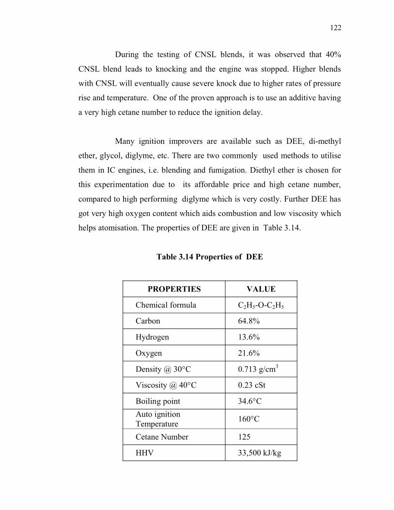
122
During the testing of CNSL blends, it was observed that 40%
CNSL blend leads to knocking and the engine was stopped. Higher blends
with CNSL will eventually cause severe knock due to higher rates of pressure
rise and temperature. One of the proven approach is to use an additive having
a very high cetane number to reduce the ignition delay.
Many ignition improvers are available such as DEE, di-methyl
ether, glycol, diglyme, etc. There are two commonly used methods to utilise
them in IC engines, i.e. blending and fumigation. Diethyl ether is chosen for
this experimentation due to its affordable price and high cetane number,
compared to high performing diglyme which is very costly. Further DEE has
got very high oxygen content which aids combustion and low viscosity which
helps atomisation. The properties of DEE are given in Table 3.14.
Table 3.14 Properties of DEE
PROPERTIES VALUE
Chemical formula C2H5-O-C2H5
Carbon 64.8%
Hydrogen 13.6%
Oxygen 21.6%
Density @ 30°C 0.713 g/cm3
Viscosity @ 40°C 0.23 cSt
Boiling point 34.6°C
Auto ignition
Temperature 160°C
Cetane Number 125
HHV 33,500 kJ/kg

123
It is observed from the table that DEE has very good properties as
required for IC engine fuel. Its flash point is -45°C and so it can be easily
fumigated at room temperature. It has a wide explosive limits in the order of
1.9 to 48 and very high cetane number. However it has a lower heat content -
25% lesser than diesel.
The first methodology is to fumigate DEE as ignition improver in
the inlet passage of the air at the inlet manifold. However it calls for very
accurate and precisely controlled pump which has to work in synchrony with
engine load which is possible only by electronic control for reliable readings.
Investigations using intravenous needle and valve could not
instantaneously respond to load/speed variations which affect the inlet
manifold pressure and variation in volumetric efficiency. So it was decided
not to go for fumigation even though it may reduce DEE consumption and
subsequent cost saving. However this can be tried out at a later date with
advanced accessories, once the performance of the DEE as ignition improver
to CNSL is proven.
The second method is to directly blend DEE with the biofuels in
calculated proportion and mix them thoroughly. This is a very accurate and
well established method and adopted in this experimentation to run higher
proportion of CNSL blends. It has been observed that CNSL has a very good
miscibility with DEE resulting in stable blends.
Four composition of CNSL blends were prepared (by volume %)
with diesel and DEE for testing and named as B10, B20, B30 and B40.
1. 15% CNSL, 5% DEE with 80% diesel denoted by B10
2. 15% CNSL, 10% DEE with 75% diesel denoted by B20

124
3. 30% CNSL, 5% DEE with 65% diesel denoted by B30
4. 30% CNSL, 10% DEE with 60% diesel denoted by B40
Performance and emission tests were conducted using DEE as
ignition improver with CNSL – diesel blends for B10 to B40 and the results
were recorded.
3.4.10 Tests with Exhaust Gas Recirculation
Exhaust gas recirculation is a method of pollution control in IC
engines by recirculating a part of the burnt gases coming out from the engine,
into the air inlet passage through a control valve as shown Figure 3.31. By
this way the major pollutant of NOx will reduce significantly due to the
dilution effect of the air fuel mixture by the burnt out gases. This results in
lesser peak temperature formed during the combustion and thereby less NOx
formation. The exhaust gases have high specific heat and more inert contents
of CO2 and nitrogen. Thus EGR reduces the oxygen content at the inlet. There
are two methods of using EGR, viz. cooled, hot.
In this investigation, exhaust gas from the engine is let into a big
tank and allowed to get cooled. A pipe is taken from this flue gas collection
tank though a control valve to regulate the quantity of the exhaust gas
admitted based on the engine load and EGR as required. CO2 concentrations
at inlet and outlet manifold are measured to calculate EGR% . The control
valve is regulated to achieve specified CO2 level for every loading.
Cooled EGR has better NOx reduction as compared to hot EGR
method, which is easy and convenient to adopt by connecting a small tube
from the tailpipe of the engine leading into the inlet air passage.

125
Figure 3.31 Exhaust gas recirculation
This investigation was carried out for 10% EGR, 15% EGR and
20% EGR setups. Readings are recorded for every EGR level as per the
standard experimental procedures as mentioned in earlier.
3.4.11 Uncertainty and Error Analysis
For any measurement there exists certain uncertainty due to
variation in the measured parameter and inherent limitations of the measuring
instruments. Further there are systematic and random errors which are to be
accounted for. So uncertainty and error analysis were carried out for the
measured parameters and given in the Appendix 7.
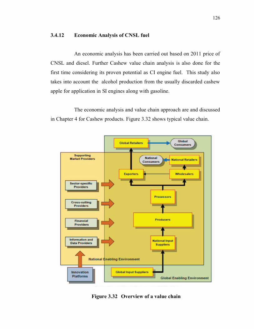
126
3.4.12 Economic Analysis of CNSL fuel
An economic analysis has been carried out based on 2011 price of
CNSL and diesel. Further Cashew value chain analysis is also done for the
first time considering its proven potential as CI engine fuel. This study also
takes into account the alcohol production from the usually discarded cashew
apple for application in SI engines along with gasoline.
The economic analysis and value chain approach are and discussed
in Chapter 4 for Cashew products. Figure 3.32 shows typical value chain.
Figure 3.32 Overview of a value chain

127
Value chain analysis is comparatively a new concept and it is superior to
supply chain analysis in many aspects. It leads to economic development and
poverty reduction. A value chain links the steps which a product takes from
the farmer to the consumer. It includes research and development, input
suppliers and finance. The farmer combines these resources with land, labour
and capital to produce commodities. In the traditional selling system farmers
produce commodities that are "pushed" into the marketplace and farmers are
isolated from the end-consumer and have little control over input costs or of
the funds received for their goods.
The value chain approach analyzes the firms in a market chain -
from input suppliers to final buyers - and the relationships factors among
them. So, Here, farmers are linked to consumers' needs, working closely with
suppliers and processors to produce the specific goods consumers demand.
Similarly, through flows of information and products, consumers are linked to
the needs of farmers. Research inputs, supportive policy and institutional
environment, availability of credit and technical support and the existence of
healthy markets and functioning infrastructure promote economy. It is also
likely to involve a wide range of key actors from farmers through to policy
makers, private-sector companies, entrepreneurs, as well as journalists.
Changing agricultural contexts, rural to urban migration, and
resulting changes for rural employment, the need for pro-poor development,
as well as a changing international scene (not least the increase in oil prices)
all indicate the importance of value-chain analysis. Cashew value chain will
eventually help farmers, cashew processing industries, users and also will
eventually lead into a new arena of renewable and affordable IC engine fuel.