chapter 3 class notes word distributions and...

Quantitative Bioinformatics

1 | P a g e

Chapter 3 Class Notes – Word Distributions and Occurrences

3.1. The Biological Problem: “restriction endonucleases provide[s] the means for precisely and reproducibly cutting the DNA into fragments of manageable size” and a “restriction map is a display of positions on a DNA molecule of locations of cleavage by one or more restriction endonucleases” – serves as a “fingerprint”. Recall that “cloning puts DNA of manageable size into vectors that allow the inserted DNA to be amplified, and the reason for doing this is that large molecules cannot be readily manipulated without breakage.” Our focus:

If we are able to digest (cut) the DNA with a restriction endonuclease such as EcoRI, approximately how many fragments would be obtained, and what would be their size distribution?

Suppose that we observe 761 occurrences of the sequence 5’-GCTGGTGG-3’ in a genome that is 50% G+C and 4.6 Mb in

size. How does this number compare with the expected number, and expected according to what model?

3.2 Modeling the Number of Restriction Sites in DNA: we know the (%G+C), and we’ll assume (for now) iid letters (and that is a

very big assumption!). Regarding the number of restriction sites, “our model is going to assume that cleavage can occur between any two successive positions on the DNA.” Even though the are not in fact independent, the “binomial distribution often works well nonetheless.” To test the iid model, we compare actual with expected: lambda DNA sequence is 48,502 bp long,


2 | P a g e

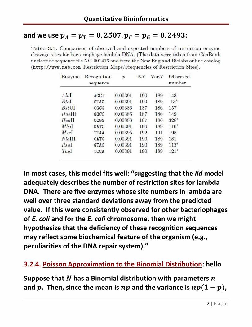
and we use :

In most cases, this model fits well: “suggesting that the iid model adequately describes the number of restriction sites for lambda DNA. There are five enzymes whose site numbers in lambda are well over three standard deviations away from the predicted value. If this were consistently observed for other bacteriophages of E. coli and for the E. coli chromosome, then we might hypothesize that the deficiency of these recognition sequences may reflect some biochemical feature of the organism (e.g., peculiarities of the DNA repair system).” 3.2.4. Poisson Approximation to the Binomial Distribution: hello

Suppose that has a Binomial distribution with parameters and . Then, since the mean is and the variance is ,


3 | P a g e

whenever is very small, the two are nearly the same. It’s not hard to show that for large and small (math language: as and so that stays constant), then the distribution for is approximately that of a Poisson RV:

The mean and variance of the Poisson distribution are

. (Note: ∑ ∑

since

∑

)

Comp. Example 3.1: estimate the probability there are no more than 2 EcoRI sites in a DNA molecule of length 10,000 assuming equal base frequencies and . Here, , and

Can be obtained in R using ppois(2,2.4). “In other words,

more than half the time, molecules of length 10,000 and uniform base frequencies will be cut by EcoRI two times or less.” 3.2.5. The Poisson Process: translate into length ( ) and into rate ( ). The mean is thus .

Moreover, provided we have two non-overlapping intervals with


4 | P a g e

, then the lengths of the intervals simply add:

3.3 Continuous Random Variables: RVs such as the Binomial and Poisson are called discrete since the RV takes on (at most countably infinite) number of points; here the RV takes values in an interval of whole real line. Further, probability formula are called probability density functions (“pdf’s”, denote ), and sums are replaced by integrals.

We already saw the uniform distribution on :

{

Here, the mean and variance are

and

The exponential distribution with parameter has pdf:

{

Here, the mean and variance are

and

The standard normal distribution has pdf:

√


5 | P a g e

Here, the mean and variance are and , and we write . Note if and , then

; equivalently,

.

We can easily use R to find Normal probabilities:

> pnorm(1.5,1,2) gives [1] 0.5987063 3.4 The Central Limit Theorem (CLT): applies to averages and

sums: are iid with mean and variance , then the

average is

. Then, the expected value and

variance of are and

, so that

√ ⁄ has expected value 0

and variance 1. The CLT states that for sufficiently large,

√ ⁄

behaves like a Standard Normal RV. This applies too to sums

since

√ ⁄

∑

√ . Next, we use this to approximate the

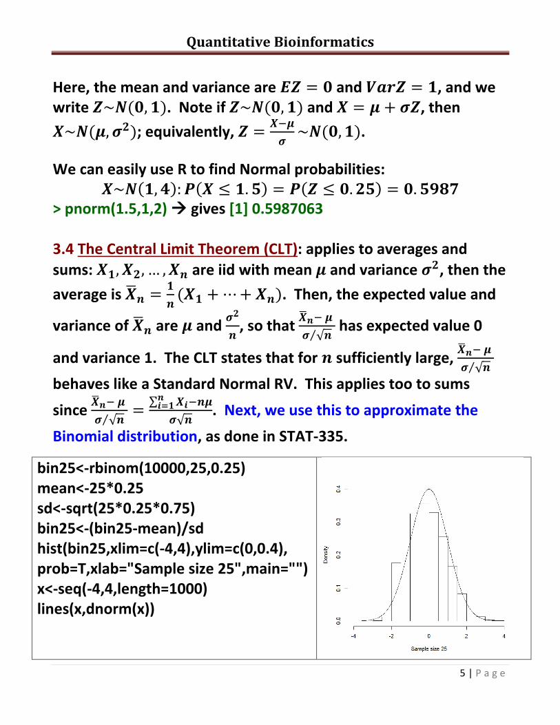
Binomial distribution, as done in STAT-335.

bin25<-rbinom(10000,25,0.25) mean<-25*0.25 sd<-sqrt(25*0.25*0.75) bin25<-(bin25-mean)/sd hist(bin25,xlim=c(-4,4),ylim=c(0,0.4), prob=T,xlab="Sample size 25",main="") x<-seq(-4,4,length=1000) lines(x,dnorm(x))


6 | P a g e

Next, continuing the previous Q: in a random uniformly distributed DNA sequence of length 1000, find the probability of at least 280 A’s. , so we

know that and

√ ; using the Normal Approximation (without the continuity correction), we get

(

)

1-pnorm((280-250)/sqrt(187.5)) gives [1] 0.01422987 3.4.1 Confidence Interval for Binomial Proportion:

For sufficiently large , since

√ ⁄ is approximately Standard

Normal, we can find a 95% CI for by using the interval:

( √

√

)

For 90%, use 1.645 in place of 1.96. See Homework Ex.10 on p.98. 3.4.2 Maximum Likelihood Estimation:

This is a technique to estimate unknown parameters such as above: we form the “likelihood” of the parameter given the data, and use basic calculus to maximize it; this gives the maximum likelihood estimate (MLE). To illustrate let be iid Bernoulli RVs with success probability ; then each probability

mass function is By independence, the joint probability function is (with ∑

)


7 | P a g e

∑ ∑

(This is the same as the likelihood for the binomial distribution

but with the ( ) term dropped since it is not a function of .)

We now view this joint probability function as the likelihood function of p and write:

We wish to find the value of which maximizes ; but this is

also the value of p which maximizes ( )

. Here, we set

. This

gives the MLE,

. See also Homework #11, p.98.

3.5 Restriction Fragment Length Distributions:

Suppose (number of restriction sites) follows a Poisson process with rate per bp; then probability of observing k sites in an

interval of length bp is

Also, if there is a site at , probability that a restriction fragment length is larger than is

( )

So, ∫

, and the density for is

(by differentiation) . So, if the number of sites ( ) follows the Poisson distribution, then the distance between the sites ( ) has an exponential ( ) distribution; mean length = .


8 | P a g e

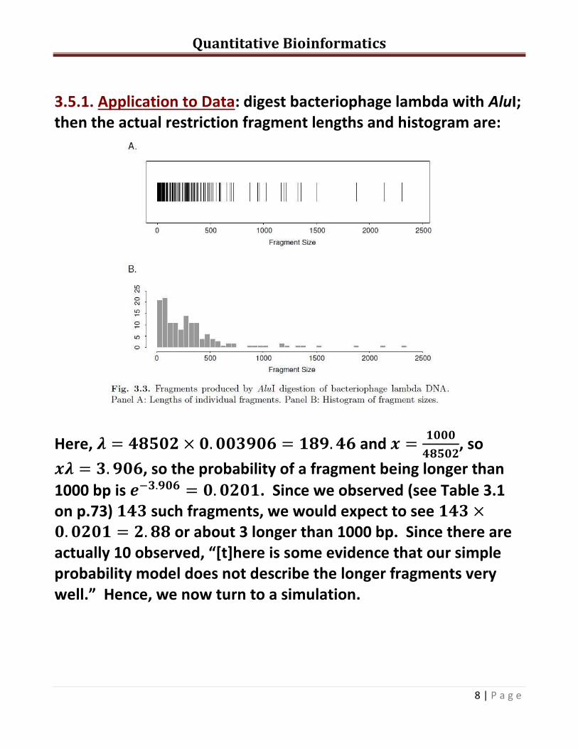
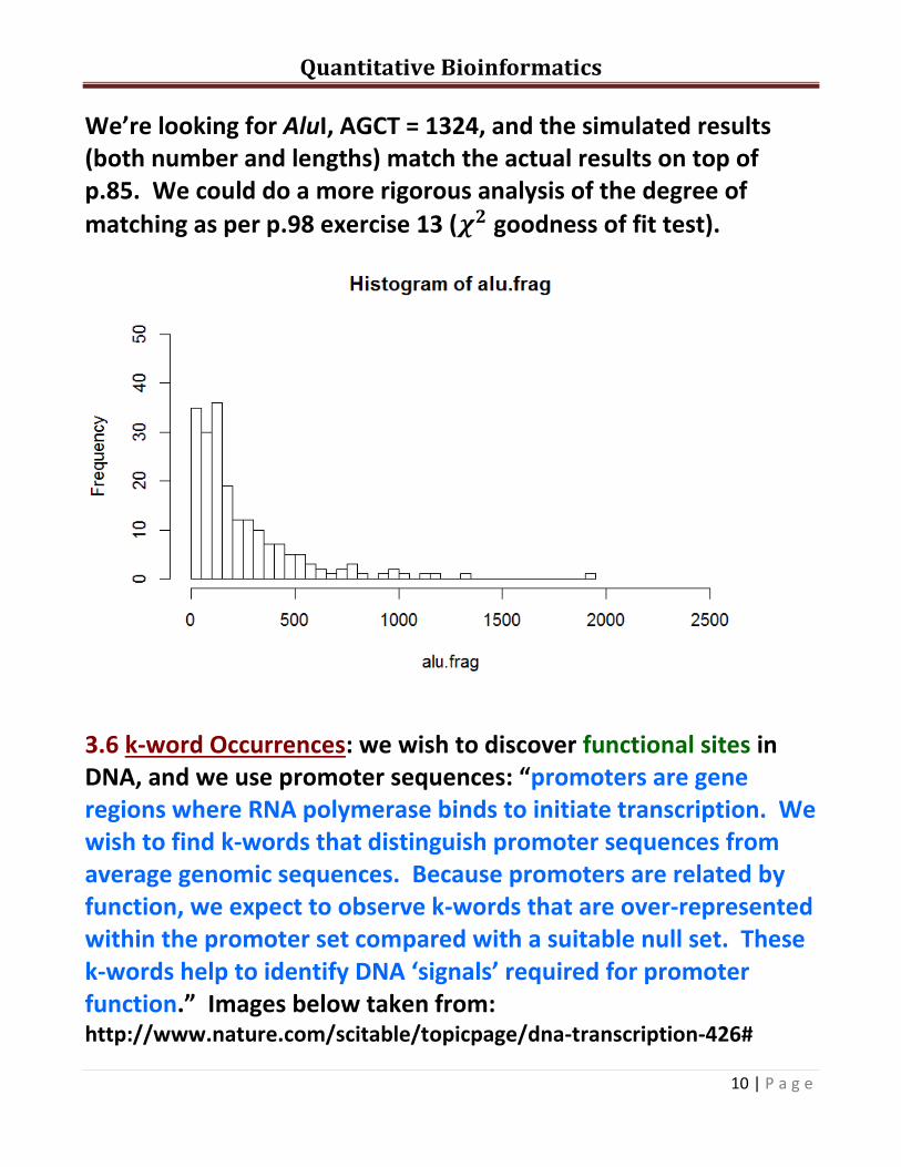
3.5.1. Application to Data: digest bacteriophage lambda with AluI; then the actual restriction fragment lengths and histogram are:

Here, and

, so

, so the probability of a fragment being longer than

1000 bp is . Since we observed (see Table 3.1 on p.73) such fragments, we would expect to see or about 3 longer than 1000 bp. Since there are actually 10 observed, “[t]here is some evidence that our simple probability model does not describe the longer fragments very well.” Hence, we now turn to a simulation.


9 | P a g e

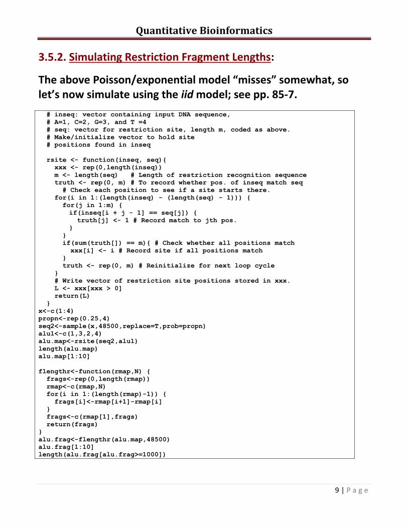
3.5.2. Simulating Restriction Fragment Lengths:

The above Poisson/exponential model “misses” somewhat, so let’s now simulate using the iid model; see pp. 85-7. # inseq: vector containing input DNA sequence,

# A=1, C=2, G=3, and T =4

# seq: vector for restriction site, length m, coded as above.

# Make/initialize vector to hold site

# positions found in inseq

rsite <- function(inseq, seq){

xxx <- rep(0,length(inseq))

m <- length(seq) # Length of restriction recognition sequence

truth <- rep(0, m) # To record whether pos. of inseq match seq

# Check each position to see if a site starts there.

for(i in 1:(length(inseq) - (length(seq) - 1))) {

for(j in 1:m) {

if(inseq[i + j - 1] == seq[j]) {

truth[j] <- 1 # Record match to jth pos.

}

}

if(sum(truth[]) == m){ # Check whether all positions match

xxx[i] <- i # Record site if all positions match

}

truth <- rep(0, m) # Reinitialize for next loop cycle

}

# Write vector of restriction site positions stored in xxx.

L <- xxx[xxx > 0]

return(L)

}

x<-c(1:4)

propn<-rep(0.25,4)

seq2<-sample(x,48500,replace=T,prob=propn)

alu1<-c(1,3,2,4)

alu.map<-rsite(seq2,alu1)

length(alu.map)

alu.map[1:10]

flengthr<-function(rmap,N) {

frags<-rep(0,length(rmap))

rmap<-c(rmap,N)

for(i in 1:(length(rmap)-1)) {

frags[i]<-rmap[i+1]-rmap[i]

}

frags<-c(rmap[1],frags)

return(frags)

}

alu.frag<-flengthr(alu.map,48500)

alu.frag[1:10]

length(alu.frag[alu.frag>=1000])


10 | P a g e

We’re looking for AluI, AGCT = 1324, and the simulated results (both number and lengths) match the actual results on top of p.85. We could do a more rigorous analysis of the degree of

matching as per p.98 exercise 13 ( goodness of fit test).

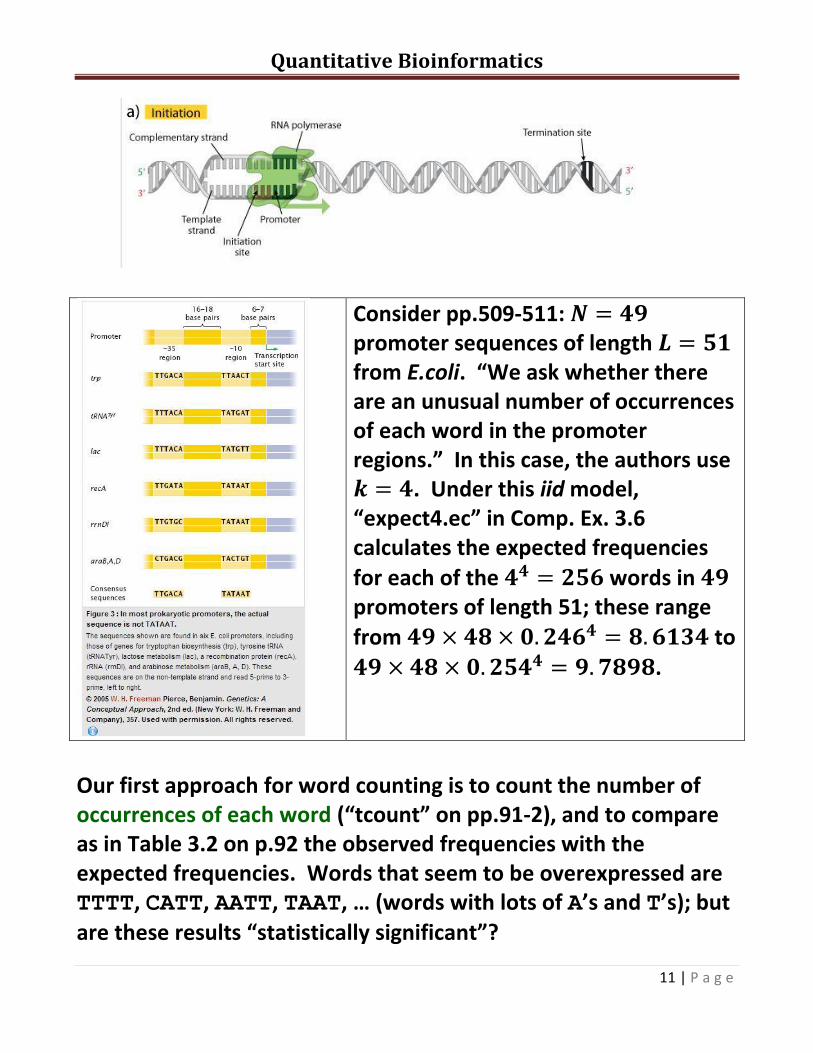
3.6 k-word Occurrences: we wish to discover functional sites in DNA, and we use promoter sequences: “promoters are gene regions where RNA polymerase binds to initiate transcription. We wish to find k-words that distinguish promoter sequences from average genomic sequences. Because promoters are related by function, we expect to observe k-words that are over-represented within the promoter set compared with a suitable null set. These k-words help to identify DNA ‘signals’ required for promoter function.” Images below taken from:

http://www.nature.com/scitable/topicpage/dna-transcription-426#


11 | P a g e

Consider pp.509-511: promoter sequences of length from E.coli. “We ask whether there are an unusual number of occurrences of each word in the promoter regions.” In this case, the authors use . Under this iid model, “expect4.ec” in Comp. Ex. 3.6 calculates the expected frequencies

for each of the words in promoters of length 51; these range

from to

.

Our first approach for word counting is to count the number of occurrences of each word (“tcount” on pp.91-2), and to compare as in Table 3.2 on p.92 the observed frequencies with the expected frequencies. Words that seem to be overexpressed are TTTT, CATT, AATT, TAAT, … (words with lots of A’s and T’s); but

are these results “statistically significant”?


12 | P a g e

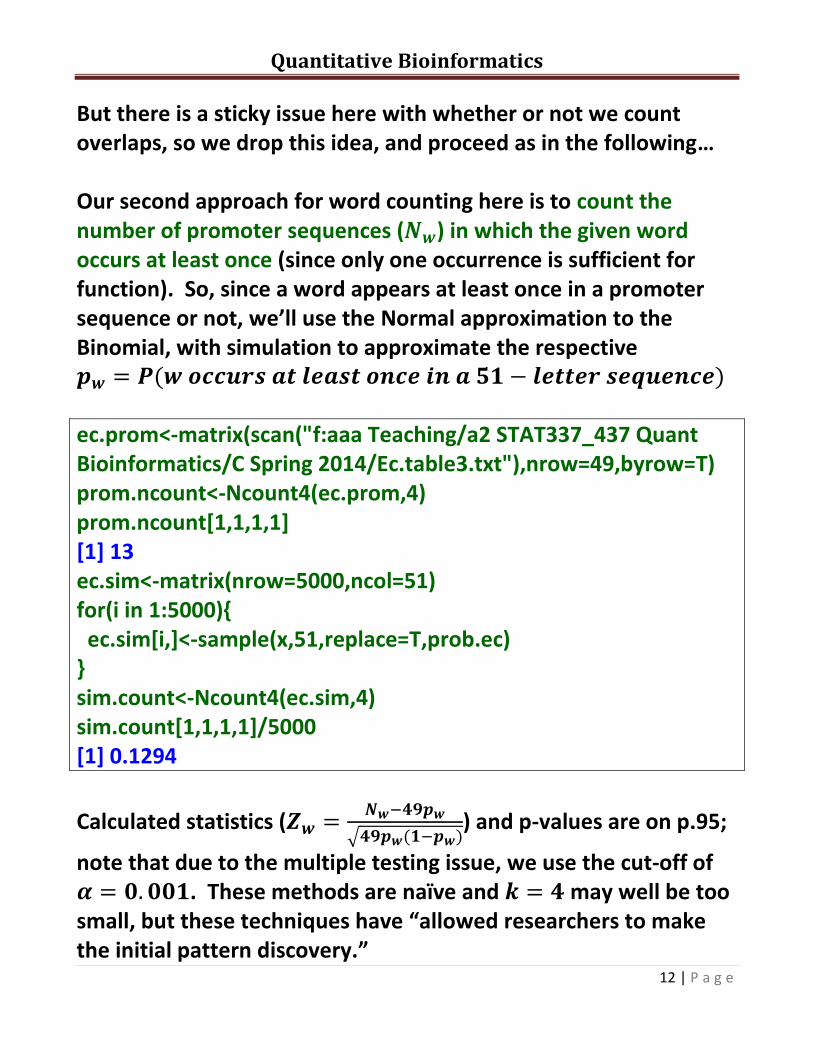
But there is a sticky issue here with whether or not we count overlaps, so we drop this idea, and proceed as in the following… Our second approach for word counting here is to count the number of promoter sequences ( ) in which the given word occurs at least once (since only one occurrence is sufficient for function). So, since a word appears at least once in a promoter sequence or not, we’ll use the Normal approximation to the Binomial, with simulation to approximate the respective ec.prom<-matrix(scan("f:aaa Teaching/a2 STAT337_437 Quant Bioinformatics/C Spring 2014/Ec.table3.txt"),nrow=49,byrow=T) prom.ncount<-Ncount4(ec.prom,4) prom.ncount[1,1,1,1] [1] 13 ec.sim<-matrix(nrow=5000,ncol=51) for(i in 1:5000){ ec.sim[i,]<-sample(x,51,replace=T,prob.ec) } sim.count<-Ncount4(ec.sim,4) sim.count[1,1,1,1]/5000 [1] 0.1294

Calculated statistics (

√ ) and p-values are on p.95;

note that due to the multiple testing issue, we use the cut-off of . These methods are naïve and may well be too small, but these techniques have “allowed researchers to make the initial pattern discovery.”

chapter 3 class notes word distributions and...

Documents