CH

AP

TE

R 3

CH

AP

TE

R 3

Ch

ap

ter 3

CH

AP

TE

R 3

CH

AP

TE

R 3

RATIONAL CONSUMER

CHOICE

McGraw-Hill/Irwin Copyright © 2011 by The McGraw-Hill Companies, Inc. All rights reserved.

Ch

ap

ter 3

3-3

Chapter Outline

• The opportunity set or budget constraint• Consumer preferences• The best feasible bundle• An application of the rational choice model

3-4

Budget Limitation

• A bundle: a particular combination of two or more goods.

• Budget constraint: the set of all bundles that exactly exhaust the consumer’s income at given prices. – Its slope is the negative of the price ratio of the

two goods.

3-5

Figure 3.1: Two Bundles of Goods

Food (kg/wk)

Shelter (sq m/wk)0

3-6

Figure 3.2: The Budget Line,or Budget Constraint

Food (kg/wk)

Shelter (sq m/wk)

3-7

Budget shifts due to price or income changes

• If the price of ONLY one good changes…– The slope of the budget constraint changes.

• If the price of both goods change by the same proportion…– The budget constraint shifts parallel to the original one.

• If income changes ….– The budget constraint shifts parallel to the original one.

3-8

Figure 3.3: The Effect of a Risein the Price of Shelter

Food (kg/wk)

Shelter (sq m/wk)

3-9

Figure 3.4: The Effect of CuttingIncome by Half

Food (kg/wk)

Shelter (sq m/wk)

3-10

Figure 3.5: The Budget Line with the Composite Good

Y (units/wk)

X (units/wk)

3-11

Figure 3.6: A Quantity Discount Gives Rise to a Nonlinear Budget Constraint

Y (R/mo)

3-12

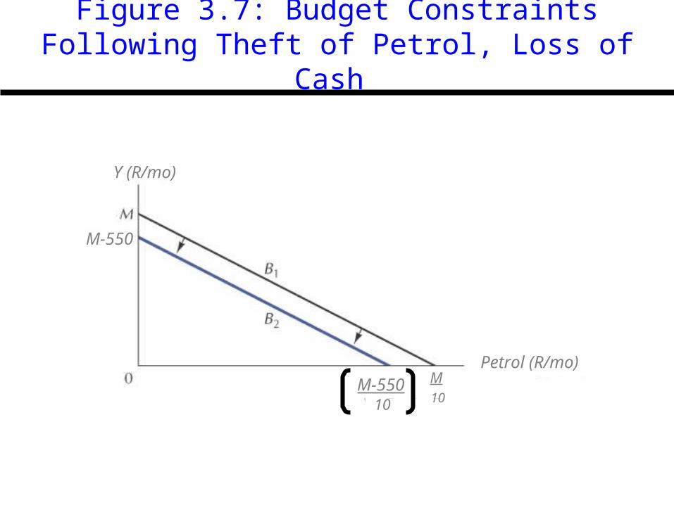
Figure 3.7: Budget Constraints Following Theft of Petrol, Loss of Cash

Petrol (R/mo)

Y (R/mo)

M-550

M10

M-55010

3-13

Properties of Preference Orderings

• Completeness: the consumer is able to rank all possible combinations of goods and services.

• More-Is-Better: other things equal, more of a good is preferred to less.

• Transitivity: for any three bundles A, B, and C, if one prefers A to B and prefers B to C, then one always prefers A to C.

• Covexity: mixtures of goods are preferable to extremes.

3-14

Figure 3.8: Generating EquallyPreferred Bundles

Food (kg/wk)

Shelter (sq m/wk)

3-15

Indifference Curves

• Indifference curve: a set of bundles among which the consumer is indifferent.

• Indifference map: a representative sample of the set of a consumer’s indifference curves, used as a graphical summary of her preference ordering.

3-16

Properties of Indifference Curves

• Indifference curves …

1. Are Ubiquitous. Any bundle has an indifference curve passing through it.

2. Are Downward-sloping. This comes from the “more-is-better” assumption.

3. Cannot cross.

4. Become less steep as we move downward and to the right along them.

This property is implied by the convexity property of preferences.

3-17

Figure 3.9: An Indifference Curve

Food (kg/wk)

Shelter (sq m/wk)0

3-18

Figure 3.10: Part of an Indifference Map

Food (kg/wk)

Shelter (sq m/wk)0

3-19

Figure 3.11: A Three-DimensionalUtility Surface

U1

U

3-20

Figure 3.12: Indifference Curvesas Projections

0

3-21

Figure 3.13: Why Two Indifference Curves Do Not Cross

Food (kg/wk)

Shelter (sq m/wk)0

3-22

Trade-offs Between Goods

• Marginal rate of substitution (MRS): the rate at which the consumer is willing to exchange the good measured along the vertical axis for the good measured along the horizontal axis.– Equal to the absolute value of the slope of the

indifference curve.

3-23

Figure 3.14: The Marginal Rateof Substitution

Food (kg/wk)

Shelter (sq m/wk)0

3-24

Figure 3.15: Diminishing MarginalRate of Substitution

Food (kg/wk)

Shelter (sq m/wk)

3-25

Figure 3.16: People with Different Tastes

Potatoes (kg/wk) Potatoes (kg/wk)

Rice (kg/wk) Rice (kg/wk)

Carlos’s

0 0

3-26

The Best Feasible Bundle

• Consumer’s Goal: to choose the best affordable bundle.– The same as reaching the highest indifference

curve she can, given her budget constraint.

– For convex indifference curves.• the best bundle will always lie at the point of tangency

between the budget line and the indifference curve.

3-27

Figure 3.17: The Best Affordable Bundle

Food (kg/wk)

Shelter (sq m/wk)

3-28

Figure 3.18: A Corner Solution

Food (kg/wk)

Shelter (sq m/wk)0

3-29

Figure 3.19: Equilibrium withPerfect Substitutes

Coke (litre/day)

Pepsi (litre/day)

3-30

Cash or Food Stamps?

• Food Stamp Program– Objective - to alleviate hunger. – How does it work?

• People whose incomes fall below a certain level are eligible to receive a specified quantity of food stamps.

• Stamps cannot be used to purchase cigarettes, alcohol, and various other items.

• The government gives food retailers cash for the stamps they accept.

3-31

Figure 3.20: Food Stamp Program vs. Cash Grant Program

R4 000 /Px R5 000 /Px

R4

00

0

R5

00

0

0

5 000

4 000

3-32

Figure 3.21: Where Food Stamps and Cash Grants Yield Different Outcomes

R4 000 /Px R5 000 /Px100 /Px

R4

000

R5

000

X (units/mo)

Y (R/mo)

40 000

50 000

3-33

Figure 3.22: How a health risk may alter consumer behaviour

0

I2

I1

K

Diet drinks

J

B

AY/Pd

Y/Ps0 Sugared drinks

I3

A

Diet drinks

BY/PS

Y/PD

Sugared drinks

K

J I3

I2

3-34

Figure 2.23: Indifference Curves forthe Utility Function U=Fs

0

3-35

Figure 2.24: Utility Along an Indifference Curve Remains Constant

0

3-36

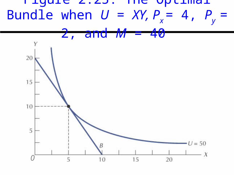
Figure 2.25: The Optimal Bundle when U = XY, Px = 4, Py = 2, and M = 40

0