chapter 3: asymptotic equipartition propertyuniversity of illinois at chicago ece 534, natasha...

University of Illinois at Chicago ECE 534, Natasha Devroye

Chapter 3: Asymptotic Equipartition Property


Chapter 3 outline

• Strong vs. Weak Typicality

• Convergence

• Asymptotic Equipartition Property Theorem

• High-probability sets and the “typical set”

• Consequences of the AEP: data compression


Strong versus Weak Typicality

• Intuition behind typicality?


Another example of Typicality

• Bit-sequences of length n = 8, prob(1) = p (prob(0) = (1-p))

• Strong typicality?

• Weak typicality?

• What if p=0.5?


Convergence of random variables


Weak Law of Large Numbers + the AEP


Typical sets intuition

• What’s the point?

• Consider iid bit-strings strings of length N=100, prob(1) = p1=0.1

• Probability of a given string X with r ones is

• Distribution of r, the # of ones in a string of length N is thus

• Number of strings with r ones is



Copyright Cambridge University Press 2003. On-screen viewing permitted. Printing not permitted. http://www.cambridge.org/0521642981

You can buy this book for 30 pounds or $50. See http://www.inference.phy.cam.ac.uk/mackay/itila/ for links.

4.4: Typicality 79

Figure 4.11. Anatomy of the typical set T . For p1 = 0.1 and N = 100 and N = 1000, these graphsshow n(r), the number of strings containing r 1s; the probability P (x) of a single stringthat contains r 1s; the same probability on a log scale; and the total probability n(r)P (x) ofall strings that contain r 1s. The number r is on the horizontal axis. The plot of log2 P (x)also shows by a dotted line the mean value of log2 P (x) = −NH2(p1) which equals −46.9when N = 100 and −469 when N = 1000. The typical set includes only the strings thathave log2 P (x) close to this value. The range marked T shows the set TNβ (as defined insection 4.4) for N = 100 and β = 0.29 (left) and N = 1000, β = 0.09 (right).

N = 100 N = 1000

n(r) =!Nr

"

0

2e+28

4e+28

6e+28

8e+28

1e+29

1.2e+29

0 10 20 30 40 50 60 70 80 90 1000

5e+298

1e+299

1.5e+299

2e+299

2.5e+299

3e+299

0 100 200 300 400 500 600 700 800 9001000

P (x) = pr1(1 − p1)N−r

0

1e-05

2e-05

0 10 20 30 40 50 60 70 80 90 100

0

1e-05

2e-05

0 1 2 3 4 5

log2 P (x)

-350

-300

-250

-200

-150

-100

-50

0

0 10 20 30 40 50 60 70 80 90 100

T

-3500

-3000

-2500

-2000

-1500

-1000

-500

0

0 100 200 300 400 500 600 700 800 9001000

T

n(r)P (x) =!N

r

"pr1(1 − p1)N−r

0

0.02

0.04

0.06

0.08

0.1

0.12

0.14

0 10 20 30 40 50 60 70 80 90 1000

0.005

0.01

0.015

0.02

0.025

0.03

0.035

0.04

0.045

0 100 200 300 400 500 600 700 800 9001000

r r



4.4: Typicality 79

Figure 4.11. Anatomy of the typical set T . For p1 = 0.1 and N = 100 and N = 1000, these graphsshow n(r), the number of strings containing r 1s; the probability P (x) of a single stringthat contains r 1s; the same probability on a log scale; and the total probability n(r)P (x) ofall strings that contain r 1s. The number r is on the horizontal axis. The plot of log2 P (x)also shows by a dotted line the mean value of log2 P (x) = −NH2(p1) which equals −46.9when N = 100 and −469 when N = 1000. The typical set includes only the strings thathave log2 P (x) close to this value. The range marked T shows the set TNβ (as defined insection 4.4) for N = 100 and β = 0.29 (left) and N = 1000, β = 0.09 (right).

N = 100 N = 1000

n(r) =!Nr

"

0

2e+28

4e+28

6e+28

8e+28

1e+29

1.2e+29

0 10 20 30 40 50 60 70 80 90 1000

5e+298

1e+299

1.5e+299

2e+299

2.5e+299

3e+299

0 100 200 300 400 500 600 700 800 9001000

P (x) = pr1(1 − p1)N−r

0

1e-05

2e-05

0 10 20 30 40 50 60 70 80 90 100

0

1e-05

2e-05

0 1 2 3 4 5

log2 P (x)

-350

-300

-250

-200

-150

-100

-50

0

0 10 20 30 40 50 60 70 80 90 100

T

-3500

-3000

-2500

-2000

-1500

-1000

-500

0

0 100 200 300 400 500 600 700 800 9001000

T

n(r)P (x) =!N

r

"pr1(1 − p1)N−r

0

0.02

0.04

0.06

0.08

0.1

0.12

0.14

0 10 20 30 40 50 60 70 80 90 1000

0.005

0.01

0.015

0.02

0.025

0.03

0.035

0.04

0.045

0 100 200 300 400 500 600 700 800 9001000

r r

• Consider iid bit-strings of length N, prob(1) = p1=0.1



• What’s the point?

• Consider iid bit-strings strings of length N=100, prob(1) = p1=0.1Copyright Cambridge University Press 2003. On-screen viewing permitted. Printing not permitted. http://www.cambridge.org/0521642981


78 4 — The Source Coding Theorem

x log2(P (x))

...1...................1.....1....1.1.......1........1...........1.....................1.......11... −50.1

......................1.....1.....1.......1....1.........1.....................................1.... −37.3

........1....1..1...1....11..1.1.........11.........................1...1.1..1...1................1. −65.91.1...1................1.......................11.1..1............................1.....1..1.11..... −56.4...11...........1...1.....1.1......1..........1....1...1.....1............1......................... −53.2..............1......1.........1.1.......1..........1............1...1......................1....... −43.7.....1........1.......1...1............1............1...........1......1..11........................ −46.8.....1..1..1...............111...................1...............1.........1.1...1...1.............1 −56.4.........1..........1.....1......1..........1....1..............................................1... −37.3......1........................1..............1.....1..1.1.1..1...................................1. −43.71.......................1..........1...1...................1....1....1........1..11..1.1...1........ −56.4...........11.1.........1................1......1.....................1............................. −37.3.1..........1...1.1.............1.......11...........1.1...1..............1.............11.......... −56.4......1...1..1.....1..11.1.1.1...1.....................1............1.............1..1.............. −59.5............11.1......1....1..1............................1.......1..............1.......1......... −46.8

.................................................................................................... −15.21111111111111111111111111111111111111111111111111111111111111111111111111111111111111111111111111111 −332.1

Figure 4.10. The top 15 stringsare samples from X100, wherep1 = 0.1 and p0 = 0.9. Thebottom two are the most andleast probable strings in thisensemble. The final column showsthe log-probabilities of therandom strings, which may becompared with the entropyH(X100) = 46.9 bits.

except for tails close to δ = 0 and 1. As long as we are allowed a tinyprobability of error δ, compression down to NH bits is possible. Even if weare allowed a large probability of error, we still can compress only down toNH bits. This is the source coding theorem.

Theorem 4.1 Shannon’s source coding theorem. Let X be an ensemble withentropy H(X) = H bits. Given ϵ > 0 and 0 < δ < 1, there exists a positiveinteger N0 such that for N > N0,

!!!!1N

Hδ(XN ) − H

!!!! < ϵ. (4.21)

4.4 Typicality

Why does increasing N help? Let’s examine long strings from XN . Table 4.10shows fifteen samples from XN for N = 100 and p1 = 0.1. The probabilityof a string x that contains r 1s and N−r 0s is

P (x) = pr1(1 − p1)N−r. (4.22)

The number of strings that contain r 1s is

n(r) ="

N

r

#. (4.23)

So the number of 1s, r, has a binomial distribution:

P (r) ="

N

r

#pr1(1 − p1)N−r. (4.24)

These functions are shown in figure 4.11. The mean of r is Np1, and itsstandard deviation is

$Np1(1 − p1) (p.1). If N is 100 then

r ∼ Np1 ±$

Np1(1 − p1) ≃ 10 ± 3. (4.25)

[Mackay textbook, pg. 78]


Definition: weak typicality


The typical set visuallyCopyright Cambridge University Press 2003. On-screen viewing permitted. Printing not permitted. http://www.cambridge.org/0521642981


4.5: Proofs 81

✲

log2 P (x)−NH(X)

TNβ

✻✻✻✻✻

0000000000000. . . 00000000000

0001000000000. . . 00000000000

0100000001000. . . 00010000000

0000100000010. . . 00001000010

1111111111110. . . 11111110111

Figure 4.12. Schematic diagramshowing all strings in the ensembleXN ranked by their probability,and the typical set TNβ.

The ‘asymptotic equipartition’ principle is equivalent to:

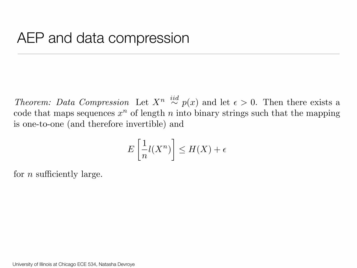
Shannon’s source coding theorem (verbal statement). N i.i.d. ran-dom variables each with entropy H(X) can be compressed into morethan NH(X) bits with negligible risk of information loss, as N → ∞;conversely if they are compressed into fewer than NH(X) bits it is vir-tually certain that information will be lost.

These two theorems are equivalent because we can define a compression algo-rithm that gives a distinct name of length NH(X) bits to each x in the typicalset.

4.5 Proofs

This section may be skipped if found tough going.

The law of large numbers

Our proof of the source coding theorem uses the law of large numbers.

Mean and variance of a real random variable are E [u] = u =!

u P (u)uand var(u) = σ2

u = E [(u − u)2] =!

u P (u)(u − u)2.

Technical note: strictly I am assuming here that u is a function u(x)of a sample x from a finite discrete ensemble X . Then the summations!

u P (u)f(u) should be written!

x P (x)f(u(x)). This means that P (u)is a finite sum of delta functions. This restriction guarantees that themean and variance of u do exist, which is not necessarily the case forgeneral P (u).

Chebyshev’s inequality 1. Let t be a non-negative real random variable,and let α be a positive real number. Then

P (t ≥ α) ≤ t

α. (4.30)

Proof: P (t ≥ α) =!

t≥α P (t). We multiply each term by t/α ≥ 1 andobtain: P (t ≥ α) ≤

!t≥α P (t)t/α. We add the (non-negative) missing

terms and obtain: P (t ≥ α) ≤!

t P (t)t/α = t/α. ✷

60 ASYMPTOTIC EQUIPARTITION PROPERTY

where the second inequality follows from (3.6). Hence

|A(n)ϵ | ≤ 2n(H(X)+ϵ). (3.12)

Finally, for sufficiently large n, Pr{A(n)ϵ } > 1 − ϵ, so that

1 − ϵ < Pr{A(n)ϵ } (3.13)

≤!

x∈A(n)ϵ

2−n(H(X)−ϵ) (3.14)

= 2−n(H(X)−ϵ)|A(n)ϵ |, (3.15)

where the second inequality follows from (3.6). Hence,

|A(n)ϵ | ≥ (1 − ϵ)2n(H(X)−ϵ), (3.16)

which completes the proof of the properties of A(n)ϵ . !

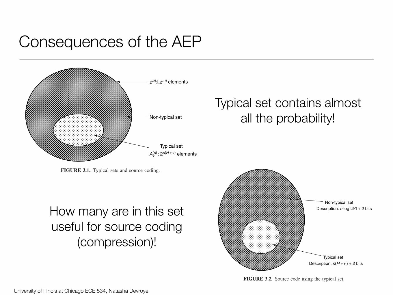
3.2 CONSEQUENCES OF THE AEP: DATA COMPRESSION

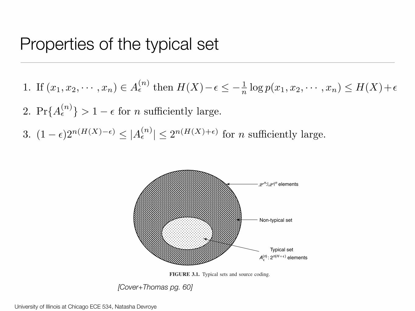
Let X1, X2, . . . , Xn be independent, identically distributed random vari-ables drawn from the probability mass function p(x). We wish to findshort descriptions for such sequences of random variables. We divide allsequences in Xn into two sets: the typical set A(n)

ϵ and its complement,as shown in Figure 3.1.

Non-typical set

Typical set

∋∋

A(n) : 2n(H + ) elements

n:| |n elements

FIGURE 3.1. Typical sets and source coding.

[Cover+Thomas pg. 60]

[Mackay pg. 81]

Bit sequences of length 100, prob(1) = 0.1

Most + least likely sequences NOT in typical set!!


Properties of the typical set



|A(n)ϵ | ≤ 2n(H(X)+ϵ). (3.12)


1 − ϵ < Pr{A(n)ϵ } (3.13)

≤!

x∈A(n)ϵ

2−n(H(X)−ϵ) (3.14)

= 2−n(H(X)−ϵ)|A(n)ϵ |, (3.15)


|A(n)ϵ | ≥ (1 − ϵ)2n(H(X)−ϵ), (3.16)





Non-typical set

Typical set

∋∋


n:| |n elements


[Cover+Thomas pg. 60]


Consequences of the AEP



|A(n)ϵ | ≤ 2n(H(X)+ϵ). (3.12)


1 − ϵ < Pr{A(n)ϵ } (3.13)

≤!

x∈A(n)ϵ

2−n(H(X)−ϵ) (3.14)

= 2−n(H(X)−ϵ)|A(n)ϵ |, (3.15)


|A(n)ϵ | ≥ (1 − ϵ)2n(H(X)−ϵ), (3.16)





Non-typical set

Typical set

∋∋


n:| |n elements


Typical set contains almost all the probability!

3.2 CONSEQUENCES OF THE AEP: DATA COMPRESSION 61

Non-typical set

Typical set

Description: n log | | + 2 bits

Description: n(H + ) + 2 bits∋

FIGURE 3.2. Source code using the typical set.

We order all elements in each set according to some order (e.g., lexi-cographic order). Then we can represent each sequence of A(n)

ϵ by givingthe index of the sequence in the set. Since there are ≤ 2n(H+ϵ) sequencesin A(n)

ϵ , the indexing requires no more than n(H + ϵ) + 1 bits. [The extrabit may be necessary because n(H + ϵ) may not be an integer.] We pre-fix all these sequences by a 0, giving a total length of ≤ n(H + ϵ) + 2bits to represent each sequence in A(n)

ϵ (see Figure 3.2). Similarly, we canindex each sequence not in A(n)

ϵ by using not more than n log |X| + 1 bits.Prefixing these indices by 1, we have a code for all the sequences in Xn.

Note the following features of the above coding scheme:

• The code is one-to-one and easily decodable. The initial bit acts asa flag bit to indicate the length of the codeword that follows.

• We have used a brute-force enumeration of the atypical set A(n)ϵ

c

without taking into account the fact that the number of elements inA(n)

ϵc is less than the number of elements in Xn. Surprisingly, this is

good enough to yield an efficient description.• The typical sequences have short descriptions of length ≈ nH .

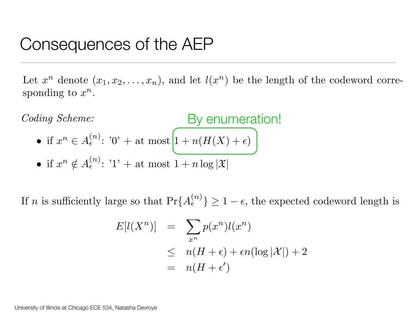
We use the notation xn to denote a sequence x1, x2, . . . , xn. Let l(xn)be the length of the codeword corresponding to xn. If n is sufficientlylarge so that Pr{A(n)

ϵ } ≥ 1 − ϵ, the expected length of the codeword is

E(l(Xn)) =!

xn

p(xn)l(xn) (3.17)

How many are in this set useful for source coding

(compression)!


Consequences of the AEP

By enumeration!


AEP and data compression


``High-probability set’’ vs. ``typical set’’

• Typical set: small number of outcomes that contain most of the probability• Is it the smallest such set?


Some notation



4.5: Proofs 81

✲

log2 P (x)−NH(X)

TNβ

✻✻✻✻✻

0000000000000. . . 00000000000

0001000000000. . . 00000000000

0100000001000. . . 00010000000

0000100000010. . . 00001000010

1111111111110. . . 11111110111

Figure 4.12. Schematic diagramshowing all strings in the ensembleXN ranked by their probability,and the typical set TNβ.

The ‘asymptotic equipartition’ principle is equivalent to:

Shannon’s source coding theorem (verbal statement). N i.i.d. ran-dom variables each with entropy H(X) can be compressed into morethan NH(X) bits with negligible risk of information loss, as N → ∞;conversely if they are compressed into fewer than NH(X) bits it is vir-tually certain that information will be lost.

These two theorems are equivalent because we can define a compression algo-rithm that gives a distinct name of length NH(X) bits to each x in the typicalset.

4.5 Proofs

This section may be skipped if found tough going.

The law of large numbers

Our proof of the source coding theorem uses the law of large numbers.

Mean and variance of a real random variable are E [u] = u =!

u P (u)uand var(u) = σ2

u = E [(u − u)2] =!

u P (u)(u − u)2.

Technical note: strictly I am assuming here that u is a function u(x)of a sample x from a finite discrete ensemble X . Then the summations!

u P (u)f(u) should be written!

x P (x)f(u(x)). This means that P (u)is a finite sum of delta functions. This restriction guarantees that themean and variance of u do exist, which is not necessarily the case forgeneral P (u).

Chebyshev’s inequality 1. Let t be a non-negative real random variable,and let α be a positive real number. Then

P (t ≥ α) ≤ t

α. (4.30)

Proof: P (t ≥ α) =!

t≥α P (t). We multiply each term by t/α ≥ 1 andobtain: P (t ≥ α) ≤

!t≥α P (t)t/α. We add the (non-negative) missing

terms and obtain: P (t ≥ α) ≤!

t P (t)t/α = t/α. ✷

[Mackay pg. 81]

Bit sequences of length 100, prob(1) = 0.1


What’s the difference?

• Why use the ``typical set’’ rather than the ``high-probability set’’?

chapter 3: asymptotic equipartition propertyuniversity of illinois at chicago ece 534, natasha...

Documents