chapter 22 eigenvalues appendix a. eigenvalue problems zengineering problems involving vibrations,...

Chapter 22Chapter 22

EigenvaluesEigenvaluesAppendix AAppendix A

Eigenvalue ProblemsEigenvalue Problems

Engineering Problems involving vibrations, elasticity, oscillating systems, etc.,

Determine the eigenvalues for n homogenous linear equations in n unknowns

}{}{][][

}{}]{[

0xIA

xxA

Non-homogeneous system

homogeneous system

reigenvecto : x ;eigenvalue :λ

Mathematical BackgroundMathematical Background

For nontrivial solutions ==>

Characteristic polynomial: det( ) = fn( )

0

0

0

0

0

x

x

x

x

aaaa

aaaa

aaaa

aaaa

x IA

n

3

2

1

nn3n2n1n

n3333231

n2232221

n1131211

0CCCCC)1( 012

22N

2N1N

1NNN

0)IAdet(

The root of fn( ) = 0 are the solutions for the eigenvalues

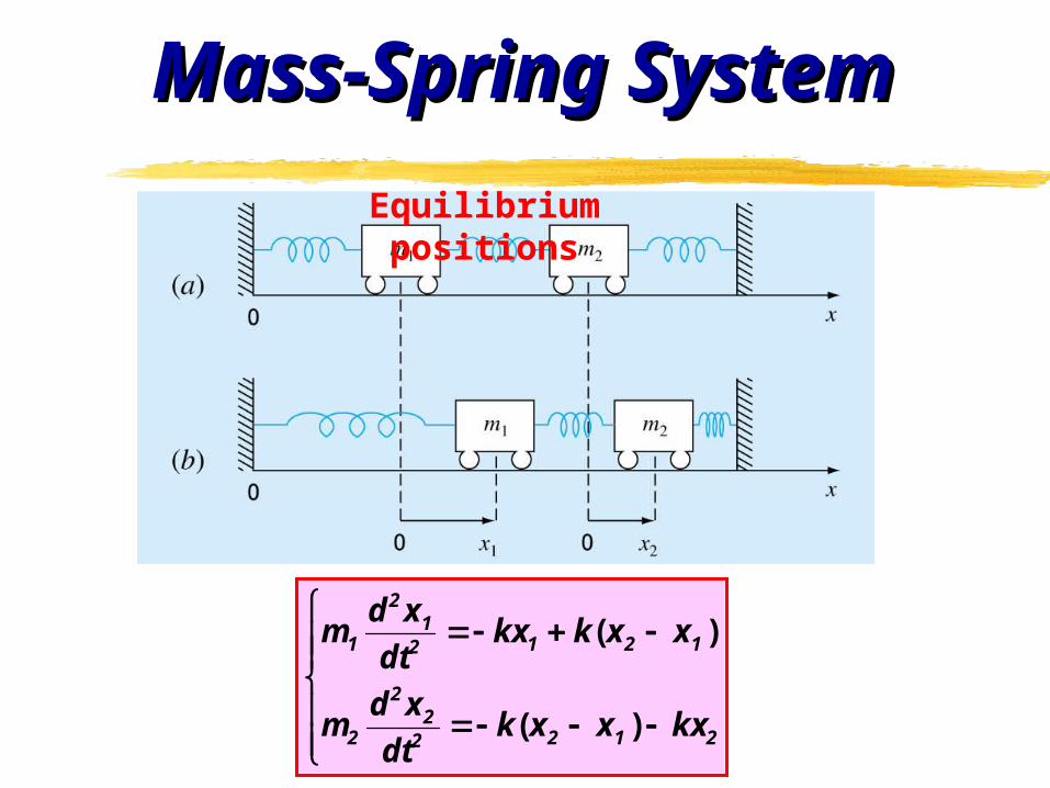
Mass-Spring SystemMass-Spring System

21222

2

2

12121

2

1

kxxxkdt

xdm

xxkkxdt

xdm

)(

)(

Equilibrium positions

Homogeneous system

Find the eigenvalues from det[ ] = 0

Mass-Spring SystemMass-Spring System

0Xm

k2X

m

k

0Xm

kX

m

k2

0x2xkdt

xdm

0xx2kdt

xdm

T

2 tXx tXx let

22

21

2

21

12

1

2122

2

2

1221

2

1

p2211

)(

)(

;sin,sin

0

0

X

X

mk2mk

mkmk2

2

1

222

22

1

//

//

m1 = m2 = 40 kg, k = 200 N/m

Characteristic equation det[ ] = 0

Two eigenvalues = 3.873s1 or 2.236 s 1

Period Tp = 2/ = 1.62 s or 2.81 s

Polynomial MethodPolynomial Method

0515 07520

105

510

mk2mk

mkmk2

2224

2

2

222

22

1

))((

)/(/

/)/(

Principal Modes of VibrationPrincipal Modes of Vibration

Tp = 1.62 s

X1 = X2

Tp = 2.81 s

X1 = X2

Buckling of ColumnBuckling of Column

Axially loaded column Buckling modes M – bending moment E – modulus of elasticity I – moment of inertia

0Ly0y

ypyEI

P

dx

yd

PyMEI

M

dx

yd

22

2

2

2

)()(

2

2

dx

ydCurvature:

Buckling of Axially Loaded ColumnBuckling of Axially Loaded Column

Eigenvalue problem

Buckling loads

Fundamental mode: n = 1

0Ly0y ypdx

yd 22

2

)()(;

2

222

L

EInEIpP

21nnpL0pLALy

0B0y

pxBpxAy

,,,sin)(

)(

cossin

2

2

critical L

EIP

Euler formula

Buckling Buckling ModesModes

2

222

L

EInEIpP

L

np


ODE

Finite-difference method

Characteristic equation: (2n)th-order polynomial

0Ly0y ;ypEI

M

dx

yd 22

2

)()(

0

0

0

0

y

y

y

y

ph2000

10

01ph210

01ph21

001ph2

0yyph2y 0yph

yy2y

n

3

2

1

22

22

22

22

1ii22

1ii2

2i

1ii1i

)(

0ph2 n22 )(det

WhichWhichScheme?Scheme?Order of Order of Errors?Errors?


One interior node (h = L/2)

Two interior nodes (h = L/3)

%)()( 10 L

22

h

2p 0yph2

Lp

a122

exact

%).%,.(,,

)(

,

317 54 L

33

L

3p 3 1ph

01ph20

0

y

y

ph21

1ph2

L

2

Lp

a

222

2

1

22

22

exact


Three interior nodes (h = L/4)

)%,.%,.(,

,)()(

,,

% 21.6 010 62 L

224 ,

L

24

L

224p

22 2ph 0ph22ph2

0

0

0

y

y

y

ph210

1ph21

01ph2

L

3

L

2

Lp

a

22322

3

2

1

22

22

22

exact

Power method for finding eigenvalues

1. Start with an initial guess for x2. Calculate w = Ax 3. Largest value (magnitude) in w is the

estimate of eigenvalue 4. Get next x by rescaling w (to avoid the

computation of very large matrix An )5. Continue until converged

Power method also gives you eigenvectors

Power MethodPower Method

Start with initial guess z = x0


Azwz

w Azw

Azwz

w Azw

)2(k

)2(

)2(k

)2()3(

)2(k

)2(k

)2()2(

)1(k

)1(

)1(k

)1()2(

)1(k

)1(k

)1()1(

k

n

k

3

k

2

k

1

n321 then , If

rescaling

k is the dominant eigenvalue


(1)0

(1) (1) (2)

(2) (2) (3)

( ) ( ) ( 1)

1. 1,1,...,1

2. ;

3. ;

...

T

k

k

k k k

normalize

n

Initial guess z x

Calculate Az w z z by biggest w

Calculate Az w z z by biggest w

Calculate

ormalize

Az w z

For large number of iterations, should converge to the largest eigenvalue

The normalization make the right hand side converges to , rather than n

Example: Power MethodExample: Power Method

1

1

1

xz

7410

438

1082

A

0)1(

01

71430

95240

21

21

15

20

1

1

1

7410

438

1082

Az 1

.

.

.)(

Start with

Assume all eigenvalues are equally important, since we don’t know which one is dominant

Consider

eigenvalue eigenvector

ExampleExample

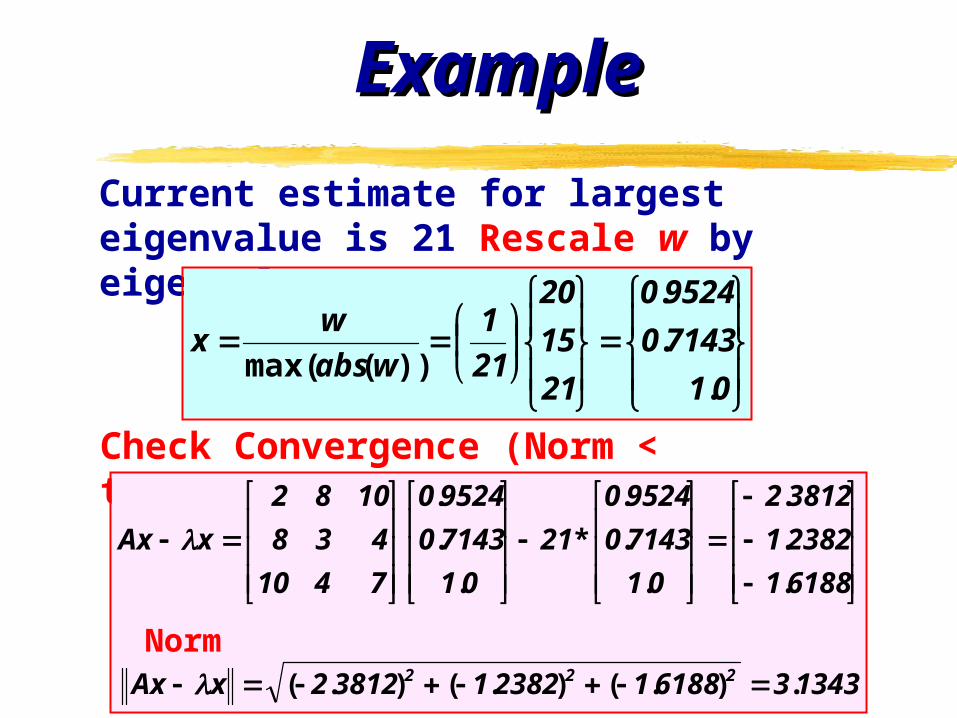
Current estimate for largest eigenvalue is 21 Rescale w by eigenvalue to get new x

01

71430

95240

21

15

20

21

1

wabs

wx

.

.

.

))(max(

Check Convergence (Norm < tol?)

13433618812382138122xAx

61881

23821

38122

01

71430

95240

21

01

71430

95240

7410

438

1082

xAx

222 .).().().(

.

.

.

.

.

.

*

.

.

.

Norm

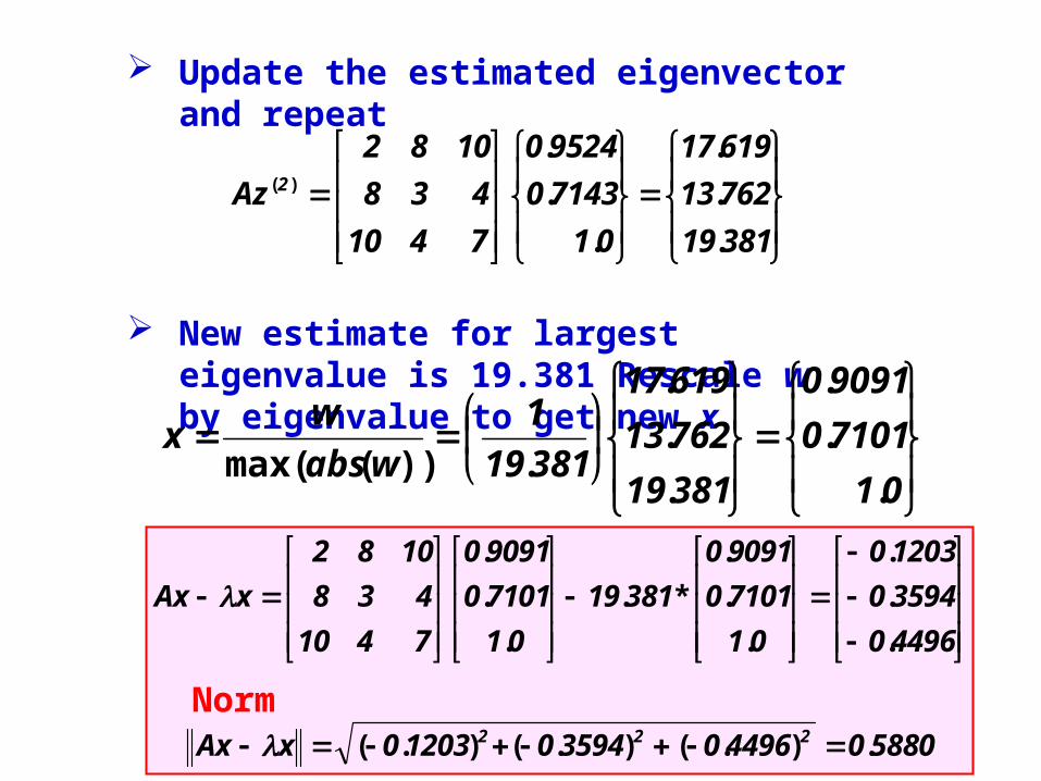
Update the estimated eigenvector and repeat

New estimate for largest eigenvalue is 19.381 Rescale w by eigenvalue to get new x

38119

76213

61917

01

71430

95240

7410

438

1082

Az 2

.

.

.

.

.

.)(

01

71010

90910

38119

76213

61917

38119

1

wabs

wx

.

.

.

.

.

.

.))(max(

58800449603594012030xAx

44960

35940

12030

01

71010

90910

38119

01

71010

90910

7410

438

1082

xAx

222 .).().().(

.

.

.

.

.

.

*.

.

.

.

Norm

ExampleExample

One more iteration

01

70800

92430

93118

93118

40313

49917

01

71010

90910

7410

438

1082

Az 3

.

.

.

.

.

.

.

.

.

.)(

18510144001153001470xAx

14400

11530

01470

01

70800

92430

93118

01

70800

92430

7410

438

1082

xAx

222 .).().().(

.

.

.

.

.

.

*.

.

.

.

Convergence criterion -- Norm (or relative error) < tol

Norm

Example: Power MethodExample: Power Method

0.1

7085.0

9200.0

030.19

030.19

482.13

507.17

0.1

7085.0

9196.0

7410

438

1082

Az

0.1

7085.0

9196.0

040.19

040.19

490.13

508.17

0.1

7084.0

9206.0

7410

438

1082

Az

0.1

7084.0

9206.0

016.19

016.19

471.13

506.17

0.1

7087.0

9181.0

7410

438

1082

Az

0.1

7087.0

9181.0

075.19

075.19

519.13

513.17

0.1

7080.0

9243.0

7410

438

1082

Az

)7(

)6(

)5(

)4(

Script file: Power_eig.mScript file: Power_eig.m

xAxNorm

» A=[2 8 10; 8 3 4; 10 4 7]A = 2 8 10 8 3 4 10 4 7» [z,m] = Power_eig(A,100,0.001);

it m z(1) z(2) z(3) z(4) z(5) 1.0000 21.0000 0.9524 0.7143 1.0000 2.0000 19.3810 0.9091 0.7101 1.0000 3.0000 18.9312 0.9243 0.7080 1.0000 4.0000 19.0753 0.9181 0.7087 1.0000 5.0000 19.0155 0.9206 0.7084 1.0000 6.0000 19.0396 0.9196 0.7085 1.0000 7.0000 19.0299 0.9200 0.7085 1.0000 8.0000 19.0338 0.9198 0.7085 1.0000 9.0000 19.0322 0.9199 0.7085 1.0000error = 8.3175e-004» zz = 0.9199 0.7085 1.0000» mm = 19.0322

» x=eig(A)x = -7.7013 0.6686 19.0327

MATLAB MATLAB Example:Example:

Power Power MethodMethod

eigenvector

eigenvalue

MATLAB function

MATLAB’s MethodsMATLAB’s Methods

e = eig(A) gives eigenvalues of A

[V, D] = eig(A) eigenvectors in V(:,k)

eigenvalues = Dii (diagonal matrix D)

[V, D] = eig(A, B) (more general eigenvalue problems) (Ax = Bx)

AV = BVD

AwxxABxw 1

Inverse Power MethodInverse Power Method

Power method give the largest eigenvalue

Inverse Power method gives the smallest

*Eigenvalues of B = A-1 are inverse of eigenvalues of A (i.e., = 1/)

So one could use power method on w = Bx to get largest eigenvalue of B - smallest of A

Calculating B is wasteful - instead use

Inverse Power MethodInverse Power Method

Basic power method gives the dominant eigenvalue Inverse power method gives the smallest eigenvalue

/1 ;x1

xABx

BxxAxAAxAx

AB ;xAx

1

111

1

smallest dominant

for eigenvaluedominant theis

1ABμ

Script file for Inverse Power Method Script file for Inverse Power Method Use LU_factor and LU_solveUse LU_factor and LU_solve

» A=[2 8 10; 8 3 4; 10 4 7]A = 2 8 10 8 3 4 10 4 7» max_it=100; tol=0.001;» [z,m] = InvPower(A,max_it,tol);L = 1.0000 0 0 4.0000 1.0000 0 5.0000 1.2414 1.0000U = 2.0000 8.0000 10.0000 0 -29.0000 -36.0000 0 0 1.6897B = 2 8 10 8 3 4 10 4 7A = 2 8 10 8 3 4 10 4 7 1.0000 12.7826 0.3000 1.0000 -0.5333it = 1 2.0000 0.7123 0.1205 1.0000 -0.8013it = 3.0000 0.6687 0.1167 1.0000 -0.8152it = 4.0000 0.6686 0.1163 1.0000 -0.8155it = 4

» zz = 0.1163 1.0000 -0.8155» mm = 0.6686» x=eig(A)x = -7.7013 0.6686 19.0327

eigenvector

eigenvalue

MATLAB function

Smallest eigenvalue

[L]

[U]

[B] = [L][U]

CVEN 302-501CVEN 302-501Homework No. 15Homework No. 15

Finish the HW but do not hand in. I will post the solution on the net.

chapter 22 eigenvalues appendix a. eigenvalue problems zengineering problems involving vibrations,...

Documents