chapter 20 – testing hypotheses about proportions · copyright 2010 pearson education, inc....
TRANSCRIPT
320 Part V From the Data at Hand to the World at Large
Chapter 20 – Testing Hypotheses about Proportions
1. Hypotheses.
a) H0 : The governor’s “negatives” are 30%. (p = 0.30)HA : The governor’s “negatives” are less than 30%. (p < 0.30)
b) H0 : The proportion of heads is 50%. (p = 0.50)HA : The proportion of heads is not 50%. (p ≠ 0.50)
c) H0 : The proportion of people who quit smoking is 20%. (p = 0.20)HA : The proportion of people who quit smoking is greater than 20%. (p > 0.20)
2. More hypotheses.
a) H0 : The proportion of high school graduates is 40%. (p = 0.40)HA : The proportion of high school graduates is not 40%. (p ≠ 0.40)
b) H0 : The proportion of cars needing transmission repair is 20%. (p = 0.20)HA : The proportion of cars needing transmission repair is less than 20%. (p < 0.20)
c) H0 : The proportion of people who like the flavor is 60%. (p = 0.60)HA : The proportion of people who like the flavor is greater than 60%. (p > 0.60)
3. Negatives.
Statement d is the correct interpretation of a P-value.
4. Dice.
Statement d is the correct interpretation of a P-value.
5. Relief.
It is not reasonable to conclude that the new formula and the old one are equally effective.Furthermore, our inability to make that conclusion has nothing to do with the P-value. Wecan not prove the null hypothesis (that the new formula and the old formula are equallyeffective), but can only fail to find evidence that would cause us to reject it. All we can sayabout this P-value is that there is a 27% chance of seeing the observed effectiveness fromnatural sampling variation if the new formula and the old one are equally effective.
6. Cars.
It is reasonable to conclude that a greater proportion of high schoolers have cars. If theproportion were no higher than it was a decade ago, there is only a 1.7% chance of seeingsuch a high sample proportion just from natural sampling variability.
7. He cheats!
a) Two losses in a row aren’t convincing. There is a 25% chance of losing twice in a row, andthat is not unusual.
b) If the process is fair, three losses in a row can be expected to happen about 12.5% of thetime. (0.5)(0.5)(0.5) = 0.125.
Copyright 2010 Pearson Education, Inc.

Chapter 20 Testing Hypotheses About Proportions 321
c) Three losses in a row is still not a convincing occurrence. We’d expect that to happenabout once every eight times we tossed a coin three times.
d) Answers may vary. Maybe 5 times would be convincing. The chances of 5 losses in a roware only 1 in 32, which seems unusual.
8. Candy.
a) P( .first three vanilla) =
≈
612
511
410
0 091
b) It seems reasonable to think there really may have been six of each. We would expect toget three vanillas in a row about 9% of the time. That’s unusual, but not that unusual.
c) If the fourth candy was also vanilla, we’d probably start to think that the mix of candieswas not 6 vanilla and 6 peanut butter. The probability of 4 vanilla candies in a row is:
P( .first four vanilla) =
≈
612
511
410
39
0 03
We would only expect to get four vanillas in a row about 3% of the time. That’s unusual.
9. Cell phones.
1) Null and alternative hypotheses should involve p, not p̂ .
2) The question is about failing to meet the goal. HA should be p < 0.96.
3) The student failed to check nq = (200)(0.04) = 8. Since nq < 10, the Success/Failurecondition is violated. Similarly, the 10% Condition is not verified.
4) SD ppq
n( ˆ)
( . )( . ). .= = ≈0 96 0 04
2000 014 The student used p̂ and q̂ .
5) Value of z is incorrect. The correct value is z = − ≈ −0 94 0 960 014
1 43. .
.. .
6) P-value is incorrect. P = P(z < –1.43) = 0.076
7) For the P-value given, an incorrect conclusion is drawn. A P-value of 0.12 provides noevidence that the new system has failed to meet the goal. The correct conclusion for thecorrected P-value is: Since the P-value of 0.076 is fairly low, there is weak evidence that thenew system has failed to meet the goal.
10. Got milk?
1) Null and alternative hypotheses should involve p, not p̂ .
2) The question asks if there is evidence that the 90% figure is not accurate, so a two-sidedalternative hypothesis should be used. HA should be p ≠ 0.90.
3) One of the conditions checked appears to be n > 10, which is not a condition for hypothesistests. The Success/Failure Condition checks np = (750)(0.90) = 675 > 10 andnq = (750)(0.10) = 75 > 10. Also, the 10% condition is not verified.
4) SD ppq
n( ˆ)
( . )( . ). .= = ≈0 90 0 10
7500 011 The student used rounded values of p̂ and q̂ .
Copyright 2010 Pearson Education, Inc.

322 Part V From the Data at Hand to the World at Large
5) Value of z is incorrect. The correct value is z = − ≈ −0 876 0 900 011
2 18. .
.. .
6) The P-value calculated is in the wrong direction. To test the given hypothesis, the lower-tail probability should have been calculated. The correct, two-tailed P-values isP = 2P(z < – 2.18) = 0.029.
7) The P-value is misinterpreted. Since the P-value is so low, there is moderately strongevidence that the proportion of adults who drink milk is different than the claimed 90%. Infact, our sample suggests that the proportion may be lower. There is only a 2.9% chance ofobserving a p̂ as far from 0.90 as this simply from natural sampling variation.
11. Dowsing.
a) H0 : The percentage of successful wells drilled by the dowser is 30%. (p = 0.30)HA : The percentage of successful wells drilled by the dowser is greater than 30%. (p > 0.30)
b) Independence assumption: There is no reason to think that finding water in one well willaffect the probability that water is found in another, unless the wells are close enough to befed by the same underground water source.Randomization condition: This sample is not random, so hopefully the customers youcheck with are representative of all of the dowser’s customers.10% condition: The 80 customers sampled may be considered less than 10% of all possiblecustomers.Success/Failure condition: np= (80)(0.30) = 24 and nq= (80)(0.70) = 56 are both greater than10, so the sample is large enough.
c) The sample of customers may not be representative of all customers, so we will proceedcautiously. A Normal model can be used to model the sampling distribution of the
proportion, with µ p̂ = =p 0.30 and σ ( ˆ)p = = ≈pq
n
( . )( . ).
0 30 0 7080
0 0512 .
We can perform aone-proportion z-test.The observed proportion ofsuccessful wells is
ˆ .p = =2780
0 3375 .
d) If his dowsing has the same success rate as standard drilling methods, there is more than a23% chance of seeing results as good as those of the dowser, or better, by natural samplingvariation.
e) With a P-value of 0.232, we fail to reject the null hypothesis. There is no evidence tosuggest that the dowser has a success rate any higher than 30%.
Copyright 2010 Pearson Education, Inc.

Chapter 20 Testing Hypotheses About Proportions 323
12. Abnormalities.
a) H0 : The percentage of children with genetic abnormalities is 5%.(p = 0.05)HA : The percentage of with genetic abnormalities is greater than 5%. (p > 0.05)
b) Independence assumption: There is no reason to think that one child having geneticabnormalities would affect the probability that other children have them.Randomization condition: This sample may not be random, but genetic abnormalities areplausibly independent. The sample is probably representative of all children, with regardsto genetic abnormalities.10% condition: The sample of 384 children is less than 10% of all children.Success/Failure condition: np= (384)(0.05) = 19.2 and nq= (384)(0.95) = 364.8 are bothgreater than 10, so the sample is large enough.
c) The conditions have been satisfied, so a Normal model can be used to model the sampling
distribution of the proportion, with µ p̂ = =p 0.05 and σ ( ˆ)p = = ≈pq
n
( . )( . ).
0 05 0 95384
0 0111.
We can perform a one-proportion z-test. The observed proportion of children with genetic
abnormalities is ˆ .p = ≈46384
0 1198.
The value of z is approximately 6.28, meaning that the observedproportion of children with genetic abnormalities is over 6 standarddeviations above the hypothesized proportion. The P-value associatedwith this z score is 2 10 10× − , essentially 0.
d) If 5% of children have genetic abnormalities, the chance of observing 46 children withgenetic abnormalities in a random sample of 384 children is essentially 0.
e) With a P-value of this low, we reject the null hypothesis. There is strong evidence thatmore than 5% of children have genetic abnormalities.
f) We don’t know that environmental chemicals cause genetic abnormalities. We merelyhave evidence that suggests that a greater percentage of children are diagnosed withgenetic abnormalities now, compared to the 1980s.
13. Absentees.
a) H0 : The percentage of students in 2000 with perfect attendance the previous month is 34%(p = 0.34)HA : The percentage of students in 2000 with perfect attendance the previous month isdifferent from 34% (p ≠ 0.34)
zp p
pq
z
z
n
=−
=−
≈
ˆ
. .
( . )( . )
.
0
0 1198 0 05
0 05 0 95
384
6 28
Copyright 2010 Pearson Education, Inc.
324 Part V From the Data at Hand to the World at Large
b) Independence assumption: It is reasonable to think that the students’ attendance recordsare independent of one another.Randomization condition: Although not specifically stated, we can assume that theNational Center for Educational Statistics used random sampling.10% condition: The 8302 students are less than 10% of all students.Success/Failure condition: np= (8302)(0.34) = 2822.68 and nq= (8302)(0.66) = 5479.32 areboth greater than 10, so the sample is large enough.
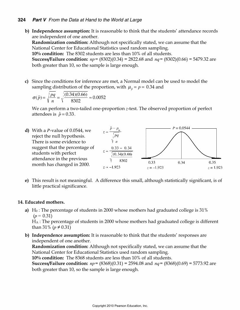
c) Since the conditions for inference are met, a Normal model can be used to model thesampling distribution of the proportion, with µ p̂ = =p 0.34 and
σ ( ˆ)p = = ≈pq
n
( . )( . ).
0 34 0 668302
0 0052
We can perform a two-tailed one-proportion z-test. The observed proportion of perfectattendees is ˆ .p = 0 33.
d) With a P-value of 0.0544, wereject the null hypothesis.There is some evidence tosuggest that the percentage ofstudents with perfectattendance in the previousmonth has changed in 2000.
e) This result is not meaningful. A difference this small, although statistically significant, is oflittle practical significance.
14. Educated mothers.
a) H0 : The percentage of students in 2000 whose mothers had graduated college is 31% (p = 0.31)HA : The percentage of students in 2000 whose mothers had graduated college is differentthan 31% (p ≠ 0.31)
b) Independence assumption: It is reasonable to think that the students’ responses areindependent of one another.Randomization condition: Although not specifically stated, we can assume that theNational Center for Educational Statistics used random sampling.10% condition: The 8368 students are less than 10% of all students.Success/Failure condition: np= (8368)(0.31) = 2594.08 and nq= (8368)(0.69) = 5773.92 areboth greater than 10, so the sample is large enough.
Copyright 2010 Pearson Education, Inc.

Chapter 20 Testing Hypotheses About Proportions 325
c) Since the conditions for inference are met, a Normal model can be used to model thesampling distribution of the proportion, with µ p̂ = =p 0.31 and
σ ( ˆ)( . )( . )
.ppq
n= = ≈
0 31 0 698368
0 0051
We can perform a one-proportiontwo-tailed z-test.The observed proportion ofstudents whose mothers are collegegraduates is ˆ .p = 0 32.
d) With a P-value of 0.048, we reject the null hypothesis. There is evidence to suggest that thepercentage of students whose mothers are college graduates has changed since 1996. Infact, the evidence suggests that the percentage has increased.
e) This result is not meaningful. A difference this small, although statistically significant, is oflittle practical significance.
15. Contributions, please, part II.
a) H0 : The contribution rate is 5% (p = 0.05)HA : The contribution rate is less than 5% (p < 0.05)
b) Independence assumption: There is no reason to believe that one randomly selectedpotential donor’s decision will affect another’s decision.Randomization condition: The sample was 100,000 randomly selected potential donors.10% condition: We will assume that the entire mailing list has over 1,000,000 names.Success/Failure condition: np= 5000 and nq= 95,000 are both greater than 10, so thesample is large enough.
The conditions have been satisfied, so a Normal model can be used to model the sampling
distribution of the proportion, with µ p̂ = =p 0.05 and σ ( ˆ)p = = ≈pq
n
( . )( . )
,.
0 05 0 95100 000
0 0007 .
We can perform a one-proportion z-test. The observed contribution rate is
ˆ,
,.p = =
4 781100 000
0 04781.
c) Since the P-value = 0.0006 islow, we reject the nullhypothesis. There is strongevidence that contribution ratefor all potential donors is lowerthan 5%.
Copyright 2010 Pearson Education, Inc.
326 Part V From the Data at Hand to the World at Large
16. Take the offer, part II.
a) H0 : The success rate is 2% (p = 0.02)HA : The success rate is something other than 2% (p ≠ 0.02)
b) Independence assumption: There is no reason to believe that one randomly selectedcardholder’s decision will affect another’s decision.Randomization condition: The sample was 50,000 randomly selected cardholders.10% condition: We will assume that the number of cardholders is more than 500,000.Success/Failure condition: np= 1000 and nq= 49,000 are both greater than 10, so thesample is large enough.
The conditions have been satisfied, so a Normal model can be used to model the sampling
distribution of the proportion, with µ p̂ = =p 0.02 and σ ( ˆ)p = = ≈pq
n
( . )( . )
,.
0 02 0 9850 000
0 0006 .
We can perform a one-proportion z-test. The observed success rate is ˆ,
,.p = =
1 18450 000
0 02368 .
c) Since the P-value is less than 0.0001, we reject the null hypothesis. There is strong evidencethat success rate for all cardholders is not 2%. In fact, this sample suggests that the successrate is higher than 2%.
17. Law School.
a) H0 : The law school acceptance rate for LSATisfaction is 63% (p = 0.63)HA : The law school acceptance rate for LSATisfaction is greater than 63% (p > 0.63)
b) Randomization condition: These 240 students may be considered representative of thepopulation of law school applicants.10% condition: There are certainly more than 2,400 law school applicants.Success/Failure condition: np = 151.2 and nq = 88.8 are both greater than 10, so the sampleis large enough.
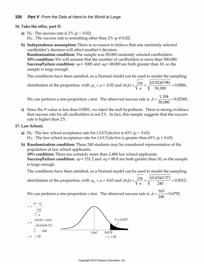
The conditions have been satisfied, so a Normal model can be used to model the sampling
distribution of the proportion, with µ p̂ = =p 0.63 and σ ( ˆ)p = = ≈pq
n
( . )( . ).
0 63 0 37240
0 0312 .
We can perform a one-proportion z-test. The observed success rate is ˆ .p = =163240
0 6792 .
Copyright 2010 Pearson Education, Inc.
Chapter 20 Testing Hypotheses About Proportions 327
c) Since the P-value = 0.057 is fairly low, we reject the null hypothesis. There is weakevidence that the law school acceptance rate is higher for LSATisfaction applicants.Candidates should decide whether they can afford the time and expense.
18. Med School.
a) H0 : The med school acceptance rate for Striving College is 46% (p = 0.46)HA : The law school acceptance rate for Striving College is less than 46% (p < 0.46)
b) Randomization condition: Assume that these 180 students are representative of allapplicants from this college.10% condition: 180 students represent less than 10% of all applicants.Success/Failure condition: np = 82.8 and nq = 97.2 are both greater than 10, so the sampleis large enough.
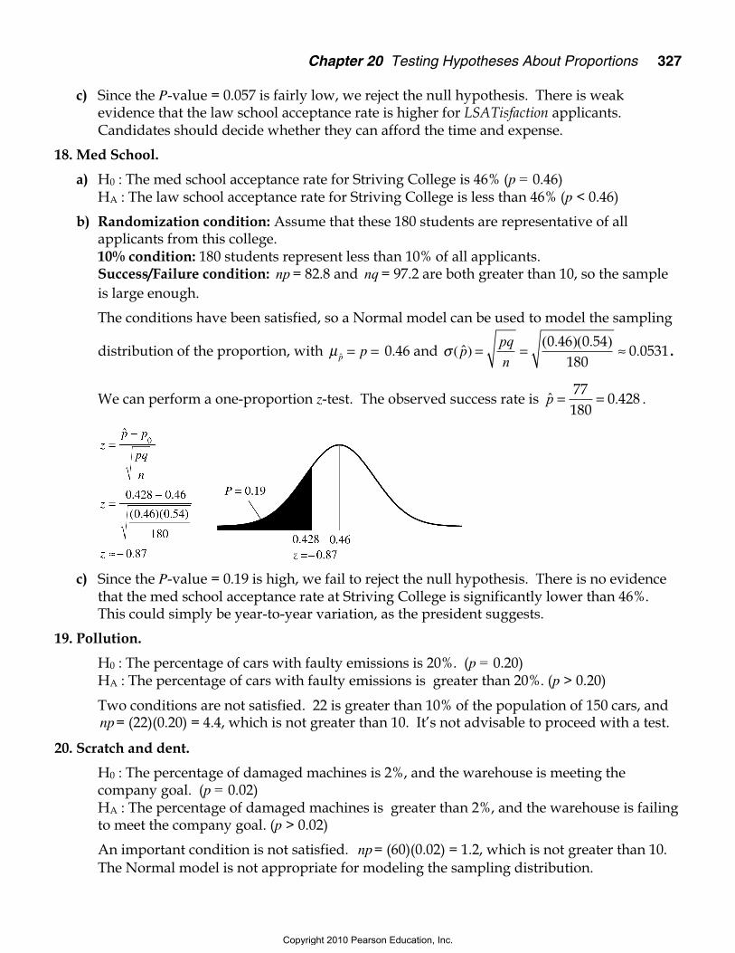
The conditions have been satisfied, so a Normal model can be used to model the sampling
distribution of the proportion, with µ p̂ = =p 0.46 and σ ( ˆ)p = = ≈pq
n
( . )( . ).
0 46 0 54180
0 0531 .
We can perform a one-proportion z-test. The observed success rate is ˆ .p = =77180
0 428 .
c) Since the P-value = 0.19 is high, we fail to reject the null hypothesis. There is no evidencethat the med school acceptance rate at Striving College is significantly lower than 46%.This could simply be year-to-year variation, as the president suggests.
19. Pollution.
H0 : The percentage of cars with faulty emissions is 20%. (p = 0.20)HA : The percentage of cars with faulty emissions is greater than 20%. (p > 0.20)
Two conditions are not satisfied. 22 is greater than 10% of the population of 150 cars, andnp= (22)(0.20) = 4.4, which is not greater than 10. It’s not advisable to proceed with a test.
20. Scratch and dent.
H0 : The percentage of damaged machines is 2%, and the warehouse is meeting thecompany goal. (p = 0.02)HA : The percentage of damaged machines is greater than 2%, and the warehouse is failingto meet the company goal. (p > 0.02)
An important condition is not satisfied. np= (60)(0.02) = 1.2, which is not greater than 10.The Normal model is not appropriate for modeling the sampling distribution.
Copyright 2010 Pearson Education, Inc.

328 Part V From the Data at Hand to the World at Large
21. Twins.
H0 : The percentage of twin births to teenage girls is 3%. (p = 0.03)HA : The percentage of twin births to teenage girls differs from 3%. (p ≠ 0.03)
Independence assumption: One mother having twins will not affect another.Observations are plausibly independent.Randomization condition: This sample may not be random, but it is reasonable to thinkthat this hospital has a representative sample of teen mothers, with regards to twin births.10% condition: The sample of 469 teenage mothers is less than 10% of all such mothers.Success/Failure condition: np= (469)(0.03) = 14.07 and nq= (469)(0.97) = 454.93 are bothgreater than 10, so the sample is large enough.
The conditions have been satisfied, so a Normal model can be used to model the sampling
distribution of the proportion, with µ p̂ = =p 0.03 and σ ( ˆ)p = = ≈pq
n
( . )( . ).
0 03 0 97469
0 0079.
We can perform a one-proportion z-test. The observed proportion of twin births to teenage
mothers is ˆ .p = ≈7469
0 015.
Since the P-value = 0.0556 isfairly low, we reject the nullhypothesis. There is someevidence that the proportion oftwin births for teenage mothersat this large city hospital islower than the proportion oftwin births for all mothers.
22. Football 2006.
H0 : The percentage of home team wins is 50%. (p = 0.50)HA : The percentage of home team wins is greater than 50%. (p > 0.50)
Independence assumption: Results of one game should not affect others.Randomization condition: This season should be representative of other seasons, withregards to home team wins.10% condition: 240 games represent less than 10% of all games, in all seasons.Success/Failure condition: np= (240)(0.50) = 120 and nq= (240)(0.50) = 120 are both greaterthan 10, so the sample is large enough.
The conditions have been satisfied, so a Normal model can be used to model the sampling
distribution of the proportion, with µ p̂ = =p 0.50 and σ ( ˆ)p = = ≈pq
n
( . )( . ).
0 5 0 5240
0 0323 .
We can perform a one-proportion z-test. The observed proportion of home team wins is
ˆ .p = =136240
0 567 .
Copyright 2010 Pearson Education, Inc.

Chapter 20 Testing Hypotheses About Proportions 329
Since the P-value = 0.02 is low,we reject the null hypothesis.There is strong evidence that theproportion of home teams winsis greater than 50%. Thisprovides evidence of a hometeam advantage.
23. Webzine.
H0 : The percentage of readers interested in an online edition is 25%. (p = 0.25)HA : The percentage of readers interested in an online edition is greater than 25%. (p > 0.25)
Independence assumption: Interest of one reader should not affect interest of otherreaders.Randomization condition: The magazine conducted an SRS of 500 current readers.10% condition: 500 readers are less than 10% of all potential subscribers.Success/Failure condition: np= (500)(0.25) = 125 and nq= (500)(0.75) = 375 are both greaterthan 10, so the sample is large enough.
The conditions have been satisfied, so a Normal model can be used to model the sampling
distribution of the proportion, with µ p̂ = =p 0.25 and σ ( ˆ)p = = ≈pq
n
( . )( . ).
0 25 0 75500
0 0194 .
We can perform a one-proportion z-test. The observed proportion of interested readers is
ˆ .p = =137500
0 274 .
Since the P-value = 0.1076 ishigh, we fail to reject the nullhypothesis. There is littleevidence to suggest that theproportion of interested readersis greater than 25%. Themagazine should not publishthe online edition.
24. Seeds.
H0 : The germination rate of the green bean seeds is 92%. (p = 0.92)HA : The germination rate of the green bean seeds is less than 92%. (p < 0.92)
Independence assumption: Seeds in a single packet may not germinate independently.They have been treated identically with regards to moisture exposure, temperature, etc.They may have higher or lower germination rates than seeds in general.Randomization condition: The cluster sample of one bag of seeds was not random.10% condition: 200 seeds is less than 10% of all seeds.Success/Failure condition: np= (200)(0.92) = 184 and nq= (200)(0.08) = 16 are both greaterthan 10, so the sample is large enough.
Copyright 2010 Pearson Education, Inc.

330 Part V From the Data at Hand to the World at Large
The conditions have not been satisfied. We will assume that the seeds in the bag arerepresentative of all seeds, and cautiously use a Normal model to model the sampling
distribution of the proportion, with µ p̂ = =p 0.92 and σ ( ˆ)p = = ≈pq
n
( . )( . ).
0 92 0 08200
0 0192 .
We can perform a one-proportion z-test. The observed proportion of germinated seeds is
ˆ .p = =171200
0 85.
Since the P-value = 0.0004 isvery low, we reject the nullhypothesis. There is strongevidence that the germinationrate of the seeds in less than92%. We should use extremecaution in generalizing theseresults to all seeds, but themanager should be safe, and avoid selling faulty seeds. The seeds should be thrown out.
25. Women executives.
H0 : The proportion of female executives is similar to the overall proportion of femaleemployees at the company. (p = 0.40)HA : The proportion of female executives is lower than the overall proportion of femaleemployees at the company. (p < 0.40)
Independence assumption: It is reasonable to think that executives at this company werechosen independently.Randomization condition: The executives were not chosen randomly, but it is reasonableto think of these executives as representative of all potential executives over many years.10% condition: 43 executives are less than 10% of all possible executives at the company.Success/Failure condition: np= (43)(0.40) = 17.2 and nq= (43)(0.60) = 25.8 are both greaterthan 10, so the sample is large enough.
The conditions have been satisfied, so a Normal model can be used to model the sampling
distribution of the proportion, with µ p̂ = =p 0.40 and σ ( ˆ)p = = ≈pq
n
( . )( . ).
0 40 0 6043
0 0747 .
We can perform a one-proportion z-test. The observed proportion is ˆ .p = ≈1343
0 302.
Since the P-value = 0.0955 ishigh, we fail to reject the nullhypothesis. There is littleevidence to suggest proportionof female executives is anydifferent from the overallproportion of 40% femaleemployees at the company.
Copyright 2010 Pearson Education, Inc.
Chapter 20 Testing Hypotheses About Proportions 331
26. Jury.
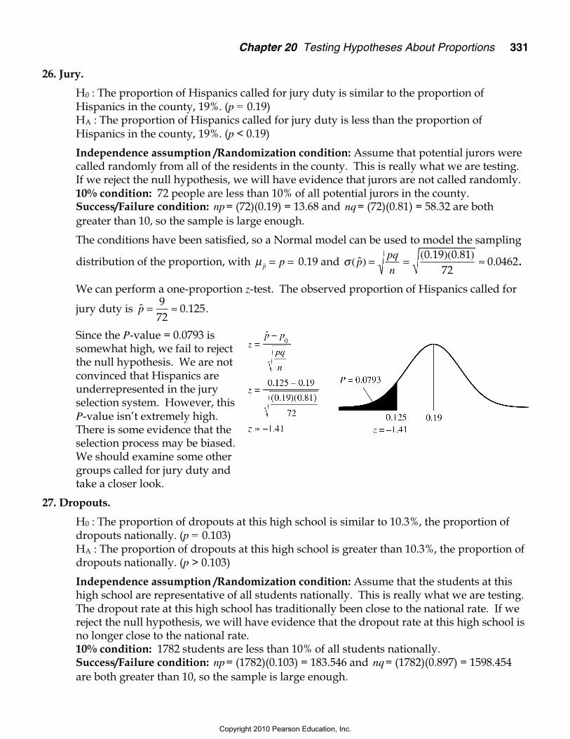
H0 : The proportion of Hispanics called for jury duty is similar to the proportion ofHispanics in the county, 19%. (p = 0.19)HA : The proportion of Hispanics called for jury duty is less than the proportion ofHispanics in the county, 19%. (p < 0.19)
Independence assumption /Randomization condition: Assume that potential jurors werecalled randomly from all of the residents in the county. This is really what we are testing.If we reject the null hypothesis, we will have evidence that jurors are not called randomly.10% condition: 72 people are less than 10% of all potential jurors in the county.Success/Failure condition: np= (72)(0.19) = 13.68 and nq= (72)(0.81) = 58.32 are bothgreater than 10, so the sample is large enough.
The conditions have been satisfied, so a Normal model can be used to model the sampling
distribution of the proportion, with µ p̂ = =p 0.19 and σ ( ˆ)p = = ≈pq
n
( . )( . ).
0 19 0 8172
0 0462.
We can perform a one-proportion z-test. The observed proportion of Hispanics called for
jury duty is ˆ .p = ≈972
0 125.
Since the P-value = 0.0793 issomewhat high, we fail to rejectthe null hypothesis. We are notconvinced that Hispanics areunderrepresented in the juryselection system. However, thisP-value isn’t extremely high.There is some evidence that theselection process may be biased.We should examine some othergroups called for jury duty andtake a closer look.
27. Dropouts.
H0 : The proportion of dropouts at this high school is similar to 10.3%, the proportion ofdropouts nationally. (p = 0.103)HA : The proportion of dropouts at this high school is greater than 10.3%, the proportion ofdropouts nationally. (p > 0.103)
Independence assumption /Randomization condition: Assume that the students at thishigh school are representative of all students nationally. This is really what we are testing.The dropout rate at this high school has traditionally been close to the national rate. If wereject the null hypothesis, we will have evidence that the dropout rate at this high school isno longer close to the national rate.10% condition: 1782 students are less than 10% of all students nationally.Success/Failure condition: np= (1782)(0.103) = 183.546 and nq= (1782)(0.897) = 1598.454are both greater than 10, so the sample is large enough.
Copyright 2010 Pearson Education, Inc.

332 Part V From the Data at Hand to the World at Large
The conditions have been satisfied, so a Normal model can be used to model the sampling
distribution of the proportion, µ p̂ = =p 0.103 and σ ( ˆ)p = = ≈pq
n
( . )( . ).
0 103 0 8971782
0 0072 .
We can perform a one-proportion z-test. The observed proportion of dropouts is
ˆ .p = ≈2101782
0 117845.
Since the P-value = 0.02 is low,we reject the null hypothesis.There is evidence that thedropout rate at this high schoolis higher than 10.3%.
28. Acid rain.
H0 : The proportion of trees with acid rain damage in Hopkins Forest is 15%, theproportion of trees with acid rain damage in the Northeast. (p = 0.15)HA : The proportion of trees with acid rain damage in Hopkins Forest is greater than 15%,the proportion of trees with acid rain damage in the Northeast. (p > 0.15)
Independence assumption /Randomization condition: Assume that the trees in HopkinsForest are representative of all trees in the Northeast. This is really what we are testing. Ifwe reject the null hypothesis, we will have evidence that the proportion of trees with acidrain damage is greater in Hopkins Forest than the proportion in the Northeast.10% condition: 100 trees are less than 10% of all trees.Success/Failure condition: np= (100)(0.15) = 15 and nq= (100)(0.85) = 85 are both greaterthan 10, so the sample is large enough.
The conditions have been satisfied, so a Normal model can be used to model the sampling
distribution of the proportion, with µ p̂ = =p 0.109 and σ ( ˆ)p = = ≈pq
n
( . )( . ).
0 15 0 85100
0 0357 .
We can perform a one-proportion z-test. The observed proportion of damaged trees is
ˆ .p = =25100
0 25 .
Since the P-value = 0.0026 islow, we reject the nullhypothesis. There is strongevidence that the trees inHopkins forest have a greaterproportion of acid rain damagethan the 15% reported for theNortheast.
Copyright 2010 Pearson Education, Inc.

Chapter 20 Testing Hypotheses About Proportions 333
29. Lost luggage.
H0 : The proportion of lost luggage returned the next day is 90%. (p = 0.90)HA : The proportion of lost luggage returned the next day is lower than 90%. (p < 0.90)
Independence assumption: It is reasonable to think that the people surveyed wereindependent with regards to their luggage woes.Randomization condition: Although not stated, we will hope that the survey wasconducted randomly, or at least that these air travelers are representative of all air travelersfor that airline.10% condition: 122 air travelers are less than 10% of all air travelers on the airline.Success/Failure condition: np= (122)(0.90) = 109.8 and nq= (122)(0.10) = 12.2 are bothgreater than 10, so the sample is large enough.
The conditions have been satisfied, so a Normal model can be used to model the sampling
distribution of the proportion, with µ p̂ = =p 0.90 and σ ( ˆ)p = = ≈pq
n
( . )( . ).
0 90 0 10122
0 0272 .
We can perform a one-proportion z-test. The observed proportion of dropouts is
ˆ .p = ≈103122
0 844 .
Since the P-value = 0.0201 islow, we reject the nullhypothesis. There is evidencethat the proportion of lostluggage returned the next day islower than the 90% claimed bythe airline.
30. TV ads.
H0 : The proportion of respondents who recognize the name is 40%.(p = 0.40)HA : The proportion of respondents who recognize the name is more than 40%. (p > 0.40)
Independence assumption: There is no reason to believe that the responses of randomlyselected people would influence others.Randomization condition: The pollster contacted the 420 adults randomly.10% condition: A sample of 420 adults is less than 10% of all adults.Success/Failure condition: np= (420)(0.40) = 168 and nq= (420)(0.60) = 252 are both greaterthan 10, so the sample is large enough.
The conditions have been satisfied, so a Normal model can be used to model the sampling
distribution of the proportion, with µ p̂ = =p 0.40 and σ ( ˆ)p = = ≈pq
n
( . )( . ).
0 40 0 60420
0 0239 .
We can perform a one-proportion z-test. The observed proportion of dropouts is
ˆ .p = ≈181420
0 431.
Copyright 2010 Pearson Education, Inc.

334 Part V From the Data at Hand to the World at Large
Since the P-value = 0.0977 isfairly high, we fail to reject thenull hypothesis. There is littleevidence that more than 40% ofthe public recognizes theproduct.Don’t run commercials duringthe Super Bowl!
31. John Wayne.
a) H0 : The death rate from cancer for people working on the film was similar to thatpredicted by cancer experts, 30 out of 220.HA : The death rate from cancer for people working on the film was higher than the ratepredicted by cancer experts.
The conditions for inference are not met, since this is not a random sample. We willassume that the cancer rates for people working on the film are similar to those predictedby the cancer experts, and a Normal model can be used to model the sampling distribution
of the rate, with µ p̂ = =p 30/220 and σ ( ˆ)p = = ( )( ) ≈pq
n
30220
190220
2200 0231. .
We can perform a one-proportion z-test. The observed cancer rate is ˆ .p = ≈46
2200 209.
Since the P-value = 0.0008 is very low, we reject the null hypothesis.There is strong evidence that the cancer rate is higher than expectedamong the workers on the film.
b) This does not prove that exposure to radiation may increase the risk of cancer. This groupof people may be atypical for reasons that have nothing to do with the radiation.
32. AP Stats.
H0 : These students achieve scores of 3 or higher at a similar rate to the nation. (p = 0.60)HA : These students achieve these scores at a different rate than the nation. (p ≠ 0.60)
Independence assumption: There is no reason to believe that students’ scores wouldinfluence others.Randomization condition: The teacher considers this class typical of other classes.10% condition: A sample of 54 students is less than 10% of all students.Success/Failure condition: np= (54)(0.60) = 32.4 and nq= (54)(0.40) = 21.6 are both greaterthan 10, so the sample is large enough.
zp p
p
z
z
=−
=−
( )( )
=
ˆ
( ˆ)
.
0
46220
30220
30220
190220
220
3 14
σ
Copyright 2010 Pearson Education, Inc.

Chapter 20 Testing Hypotheses About Proportions 335
The conditions have been satisfied, so a Normal model can be used to model the sampling
distribution of the proportion, with µ p̂ = =p 0.60 and σ ( ˆ)p = = ≈pq
n
( . )( . ).
0 60 0 4054
0 0667 .
We can perform a one-proportion z-test. The observed pass rate is ˆ .p = 0 65 .
Since the P-value = 0.453 is high,we fail to reject the null hypothesis.There is little evidence that the rateat which these students score 3 orhigher on the AP Stats exam is anyhigher than the national rate.
The teacher has no cause to brag. Her students did have a higher rate of scores of 3 orhigher, but not so high that the results could not be attributed to sampling variability.
Copyright 2010 Pearson Education, Inc.