chapter 20 global climate change - who
TRANSCRIPT

SummaryAccumulating evidence suggests that the global climate (i.e. conditionsmeasured over 30 years or longer) is now changing as a result of humanactivities—most importantly, those which cause the release of greenhousegases from fossil fuels. The most recent report (2001) from the UnitedNations’ Intergovernmental Panel on Climate Change (IPCC) estimatesthat the global average land and sea surface temperature has increasedby 0.6±0.2 ∞C since the mid-19th century, with most change occurringsince 1976. Patterns of precipitation have also changed: arid and semi-arid regions are becoming drier, while other areas, especially mid-to-highlatitudes, are becoming wetter. Where precipitation has increased, therehas been a disproportionate increase in the frequency of the heaviest pre-cipitation events. Based on a range of alternative development scenariosand model parameterizations, the IPCC concluded that if no specificactions were taken to reduce greenhouse gas emissions, global tempera-tures would be likely to rise between 1.4 and 5.8 ∞C from 1990 to 2100.Predictions for precipitation and wind speed were less consistent, butalso suggested significant changes.
Risks to human health from climate change would arise through avariety of mechanisms. In this chapter, we have used existing or newmodels that describe observed relationships between climate variations,either over short time periods or between locations, and a series of healthoutcomes. These climate–health relationships were linked to alternativeprojections of climate change, related to unmitigated future emissions ofgreenhouse gases, and two alternative scenarios for greenhouse gas emis-sions. Average climate conditions during the period 1961–1990 wereused as a baseline, as anthropogenic effects on climate are consideredmore significant after this period. The resulting models give estimates of the likely future effects of climate change on exposures to thermalextremes and weather disasters (deaths and injuries associated with
Chapter 20
Global climate change
Anthony J. McMichael,Diarmid Campbell-Lendrum, Sari Kovats,Sally Edwards, Paul Wilkinson, Theresa Wilson,Robert Nicholls, Simon Hales, Frank Tanser,David Le Sueur, Michael Schlesinger and Natasha Andronova

floods), the distribution and incidence of malaria, the incidence of diar-rhoea, and malnutrition (via effects on yields of agricultural crops). Asthere is considerable debate over the extent to which such short-termrelationships will hold true under the longer-term processes of climatechange, we made adjustments for possible changes in vulnerability, eitherthrough biological or socioeconomic adaptation. Estimates of futureeffects were interpolated back to give an approximate measure of theeffects of the climate change that have occurred since 1990 on the burdenof disease in 2000.
The effects considered here represent only a subset of the ways inwhich climate change may affect health. Other potential consequencesinclude influences of changing temperature and precipitation on otherinfectious diseases (including the possible emergence of new pathogens),the distribution and abundance of agricultural pests and pathogens,destruction of public health infrastructure, and the production of pho-tochemical air pollutants, spores and pollens. Rising sea levels may causesalination of coastal lands and freshwater supplies, resulting in popula-tion displacements. Changes in the availability and distribution ofnatural resources, especially water, may increase risk of drought, famineand conflict.
Our analyses suggested that climate change will bring some healthbenefits, such as lower cold-related mortality and greater crop yields intemperate zones, but these will be greatly outweighed by increased ratesof other diseases, particularly infectious diseases and malnutrition indeveloping regions. We estimated a small proportional decrease in car-diovascular and respiratory disease mortality attributable to climateextremes in tropical regions, and a slightly larger benefit in temperateregions, caused by warmer winter temperatures. As there is evidence thatsome temperature-attributable mortality represents small displacementsof deaths that would occur soon in any case, no assessment was madeof the associated increase or decrease in disease burden. Climate changewas estimated to increase the relative risk of diarrhoea in regions madeup mainly of developing countries to approximately 1.01–1.02 in 2000,and 1.08–1.09 in 2030. Richer countries (gross domestic product [GDP]>US$6000/year), either now or in the future, were assumed to sufferlittle or no additional risk of diarrhoea. This modest change in relativerisk relates to a major cause of ill-health, so that the estimated associ-ated disease burden in 2000 is relatively large (47000 deaths and 1.5million disability-adjusted life years [DALYs]). Effects on malnutritionvaried markedly even across developing subregions,1 from large increasesin SEAR-D (RR=1.05 in 2000, and 1.17 in 2030) to no change or aneventual small decrease in WPR-B. Again, these are small relativechanges to a large disease burden, giving an estimated 77000 deaths and2.8 million DALYs in 2000. We calculated much larger proportionalchanges in the numbers of people killed in coastal floods (RR in EUR-Bof up to 1.8 in 2000, and 6.3 in 2030), and inland floods (RR in AMR-
1544 Comparative Quantification of Health Risks

A of up to 3.0 in 2000, and 8.0 in 2030). Although the proportionalchange is much larger than for other health outcomes, the baselinedisease burden is much lower. The aggregate health effect in 2000 istherefore comparatively small (2000 deaths and 193000 DALYs). Weestimated relatively large changes in the relative risk of falciparummalaria in countries at the edge of the current distribution. However,most of the estimated attributable disease burden (27000 deaths and 1million DALYs) is associated with small proportional changes in regionsthat are already highly endemic, principally in Africa.
Overall, the effects of global climate change are predicted to be heavilyconcentrated in poorer populations at low latitudes, where the mostimportant climate-sensitive health outcomes (malnutrition, diarrhoeaand malaria) are already common, and where vulnerability to climateeffects is greatest. These diseases mainly affect younger age groups, sothat the total burden of disease due to climate change appears to be bornemainly by children in developing countries.
Considerable uncertainties surround these estimates. These stempartly from the complexity of climate models, partly from gaps in reliable data on which to base climate–health relationships, and, mostimportantly, from uncertainties around the degree to which currentclimate–health relationships will be modified by biological and socioe-conomic adaptation in the future. These uncertainties could be reducedin subsequent studies by (i) applying projections from several climatemodels; (ii) relating climate and disease data from a wider range of climatic and socioeconomic environments; (iii) more careful validationagainst patterns in the present or recent past; and (iv) more detailed longitudinal studies of the interaction of climatic and non-climatic influences on health.
1. Introduction
1.1 Evidence for climate change in the recent past andpredictions for the future
Humans are accustomed to climatic conditions that vary on daily, sea-sonal and inter-annual time-scales. Accumulating evidence suggests thatin addition to this natural climate variability, average climatic conditionsmeasured over extended time periods (conventionally 30 years or longer)are also changing, over and above the natural variation observed ondecadal or century time-scales. The causes of this climate change areincreasingly well understood. Climatologists have compared climatemodel simulations of the effects of greenhouse gas (GHG) emissionsagainst observed climate variations in the past, and evaluated possiblenatural influences such as solar and volcanic activity. They concludedthat “. . . there is new and stronger evidence that most of the warmingobserved over the last 50 years is likely to be attributable to human activities” (IPCC 2001b).
Anthony J. McMichael et al. 1545

The Third Assessment Report of the IPCC (IPCC 2001b) estimatesthat globally the average land and sea surface temperature has increasedby 0.6±0.2 ∞C since the mid-19th century, with much of the changeoccurring since 1976 (Figure 20.1). Warming has been observed in allcontinents, with the greatest temperature changes occurring at middleand high latitudes in the Northern Hemisphere. Patterns of precipitationhave also changed: arid and semi-arid regions are apparently becomingdrier, while other areas, especially mid-to-high latitudes, are becomingwetter. Where precipitation has increased, there has also been a dispro-portionate increase in the frequency of the heaviest precipitation events(Karl and Knight 1998; Mason et al. 1999). The small amount of cli-matic change that has occurred so far has already had demonstrableeffects on a wide variety of natural ecosystems (Walther et al. 2002).
Climate model simulations have been used to estimate the effects ofpast, present and likely future GHG emissions on climate changes. Thesemodels are primarily based on data on the heat-retaining properties ofgases released into the atmosphere from natural and anthropogenic(man-made) sources, as well as the measured climatic effects of othernatural phenomena, as described above. The models used by the IPCChave been validated by “back-casting”—that is, testing their ability toexplain climate variations that already occurred in the past. In general,the models are able to give good approximations of past patterns only
1546 Comparative Quantification of Health Risks
Figure 20.1 Observed global average land and sea surface temperaturesfrom 1860 to 2000
Source: Climatic Research Unit, Norwich, England.
Observations
30-year running average
Glo
bal-m
ean
tem
pera
ture
ano
mal
y (°C
)
1860 1880 1900 1920 1940 1960 1980 2000
Year AD
Average1961–1990
0.6
0.4
0.2
–0.2
–0.4
–0.6
0.0

when anthropogenic emissions of non-GHG air pollutants (particulates,dust, oxides of sulfur, etc.) are included along with natural phenomena(IPCC 2001b). This emphasizes that (i) the models represent a goodapproximation of the climate system; (ii) natural variations are impor-tant contributors to climatic variations, but cannot adequately explainpast trends on their own; and (iii) anthropogenic GHG emissions are animportant contributor to climate patterns, and are likely to remain so inthe future.
Considering a range of alternative economic development scenariosand model parameterizations, the IPCC concluded that if no specificactions were taken to reduce GHG emissions, global temperatures wouldrise between 1.4 and 5.8 ∞C from 1990 to 2100. The projections for pre-cipitation and wind speed are less consistent in terms of magnitude andgeographical distribution, but also suggest significant changes in bothmean conditions and in the frequency and intensity of extreme events(Table 20.1).
1.2 Estimating the effects of climate change on health
Human health is sensitive to temporal and geographical variations inweather (short-term fluctuations in meteorological conditions) andclimate (longer-term averages of weather conditions). Weather has nothistorically been considered as subject to alteration by human actions,although its effects may be lessened by adaptation measures (e.g. Kovatset al. 2000b). While adaptation is also a very important determinant ofthe health consequences of climate change, the effect of anthropogenicGHG emissions on climate means that climate change can in principlebe considered a risk factor that could potentially be altered by humanintervention, with associated effects on the burden of disease.
The effects of GHG emissions on human health differ somewhat fromthe effects of other risk factors in that they are mediated by a diversityof causal pathways (e.g. Figure 20.2; McMichael et al. 1996; Patz et al.2000; Reiter 2000) and eventual outcomes, typically long delays betweencause and effect, and great difficulties in eliminating or substantiallyreducing the risk factors. An additional challenge is that climate changeoccurs against a background of substantial natural climate variability,and its health effects are confounded by simultaneous changes in manyother influences on population health (Kovats et al. 2001; Reiter 2001;Woodward et al. 1998). Empirical observation of the health conse-quences of long-term climate change, followed by formulation, testingand then modification of hypotheses would therefore require long time-series (probably several decades) of careful monitoring. While thisprocess may accord with the canons of empirical science, it would notprovide the timely information needed to inform current policy decisionson GHG emission abatement, so as to offset possible health conse-quences in the future. Nor would it allow early implementation of policies for adaptation to climate changes, which are inevitable owing
Anthony J. McMichael et al. 1547

to both natural variations and past GHG emissions. Therefore, the bestestimation of the future health effects of climate change will necessarilycome from modelling based on current understanding of the effects ofclimate (not weather) variation on health from observations made in thepresent and recent past, acknowledging the influence of a large range ofmediating factors.
Since the early 1990s, IPCC Working Group II has collated some ofthe accumulating predictions of climate effects on health (IPCC 2001a).The health effects of climate variability and change have also beenreviewed by a national committee in the United States of America
1548 Comparative Quantification of Health Risks
Table 20.1 Estimates of confidence in observed and projected changesin extreme weather and climate events
Confidence in projectedConfidence in observed changes (during
Changes in phenomenon changes (latter half of 1900s) the 21st century)
Higher maximum temperatures Likelya Very likelya
and more hot days over nearly all land areas
Higher minimum temperatures, Very likelya Very likelya
fewer cold days and frost days over nearly all land areas
Reduced diurnal temperature Very likelya Very likelya
range over most land areas
Increase of heat indexb over Likely,a over many areas Very likely,a over most land areas areas
More intense precipitation Likely,a over many northern Very likely,a over many eventsa hemisphere mid- to high- areas
latitude land areas
Increased summer continental Likely,a in a few areas Likely,a over most drying and associated risk of mid-latitude continental drought interiors. (Lack of
consistent projections inother areas)
Increase in tropical cyclone peak Not observed in the few Likely,a over some areaswind intensitiesc analyses available
Increase in tropical cyclone Insufficient data for Likely,a over some areasmean and peak precipitation assessmentintensitiesd
a Judgement estimates for confidence: virtually certain (greater than 99% chance that the result istrue); very likely (90–99% chance); likely (66–90% chance); medium likelihood (33–66% chance);unlikely (10–33% chance); very unlikely (1–10% chance); exceptionally unlikely (less than 1% chance).
b Past and future changes in tropical cyclone location and frequency are uncertain.c For other areas, there are either insufficient data or conflicting analyses.d Based on warm season temperature and humidity.
Source: Adapted from IPCC (2001b).

(National Research Council 2001a) and, more recently, in a book by theWorld Health Organization (WHO) (McMichael et al. 2003). As yet,however, there has been no concerted attempt to integrate these variousresearch findings into a single standardized estimate of the likely nethealth effects of climate change, nor to estimate the possible health gainsassociated with different mitigation and amelioration strategies. In addi-tion to the uncertainties of future climate projections, there are severalobstacles to achieving this aim.
• Not all of the probable health outcomes have been modelled, oftendue to lack of parameterization data and the complexity of causalpathways. Modelling efforts so far have tended to concentrate onthose causal relationships that can more easily be modelled, ratherthan those with the potentially greatest effects (e.g. extreme temper-atures on cardiovascular disease mortality, rather than sea-level riseon the health of displaced populations).
• Little emphasis has been given to the validation of models relatingclimate change to health. Validation would provide a basis for makinguncertainty estimates around projections, and would afford an objec-tive criterion for choosing between different models or modellingapproaches.
Anthony J. McMichael et al. 1549
Figure 20.2 Pathways through which climate change may affect health
Source: Adapted from Patz et al. (2000).
Air pollution
levels
Contamination
pathways
Transmission dynamics
Natural ecosystems
and agriculture
Health effects
Temperature-relatedillness, death
Extreme weather-related health effects
Air pollution-relatedhealth effects
Water- and food-bornediseases
Vector- and rodent-borne diseases
Effects of food and water
shortages
Effects of populationdisplacement
Adaptation
measures
Moderating influences
Globalclimatechange
Regionalweatherchanges:
- heatwaves
- extremeweather
- temperature
- precipitation

• Adaptations to climate change (i.e. autonomous or planned responsesthat reduce the vulnerability of populations to the consequences ofclimate change) are often not addressed.
• Interactions between the effects of climate change and other changesto human populations (e.g. investment in health infrastructure, leveland equity of distribution of wealth) are seldom explicitly estimated.
• The various disease-specific models invariably generate outputs in dif-ferent units, which may be only indirectly related to disease burden(e.g. populations at risk of disease transmission, rather than diseaseincidence). This hampers estimation of the aggregated health impactsof different scenarios.
• Little effort has previously been directed to describing and under-standing the geographical variations in likely impacts.
The first four obstacles are likely to be at least partially addressed inthe future, as disease-specific models become more sophisticated and,perhaps more importantly, through the accumulation of greater quanti-ties of reliable data for model parameterization and testing. In thischapter, we have estimated the relative risk of a series of health outcomesunder a range of scenarios of climate change, variously mitigated byreducing GHG emissions. In all cases, care was taken to describe explic-itly the scientific basis for our estimation, the assumptions that were builtinto the quantitative models, and to give realistic uncertainty estimatesaround projections. Later sections describe ways in which specific diseasemodels may be improved.
2. Risk factor definition and measurement
2.1 Definitions of risk factor and exposure scenarios
The risk factor was defined as current and future changes in globalclimate attributable to increasing atmospheric concentrations of green-house gases (GHGs).
Composite climate scenarios are adopted instead of the (more prefer-able) continuous measurements of individual climate variables because(i) climate is a multivariate phenomenon, including temperature, precip-itation, wind speed, etc., and therefore cannot be measured on a singlescale; (ii) climate changes will vary significantly with geography and time:these are not fully captured in global averages of climate variables; and(iii) all aspects of climate are likely to be altered by GHG levels in theatmosphere.
The exposure categories considered here are global climate scenariosresulting at specified points in time over the coming half-century from:
1. unmitigated emissions trends, that is, approximately following theIPCC IS92a scenario;
1550 Comparative Quantification of Health Risks

2. emissions reduction, resulting in stabilization at 750ppm CO2 equiv-alent by the year 2210 (s750);
3. more severe emissions reduction, resulting in stabilization at 550ppmCO2 equivalent by the year 2170 (s550);
4. average climate conditions for 1961–1990, the World MeteorologicalOrganization (WMO) climate normal (baseline).
Although future GHG emissions are inherently uncertain, the un-mitigated emissions scenario adopted here was, until recently, the IPCCmid-range projection, and was very widely used in climate impact model-ling. The stabilization categories used here represent plausible, though economically and technically challenging, projections that are dependenton there being major efforts to curtail emissions. Estimated changes inCO2 concentrations, and associated changes in global temperature andsea level, are shown in Table 20.2 and Figure 20.3. Although alternativeemissions scenarios for climate stabilization are available, they have notbeen applied to a wide range of impact models.
We do not attempt to estimate all health outcomes of specificpolicy/development pathways through which these, or other, GHG levelscould be achieved: for example, compliance with the Kyoto Protocol of the United Nations Framework Convention on Climate Change(UNFCCC), or of the world following one or other of the IPCC SpecialReport on Emissions Scenarios (SRES)—both of which also includedescriptions of alternative future global socioeconomic development scenarios. The costs or additional benefits of specific interventions to
Anthony J. McMichael et al. 1551
Table 20.2 Successive measured and modelled CO2 concentrations,global mean temperature and sea-level rise associated withalternative emissions scenarios
1961–90 1990s 2020s 2050s
Carbon dioxide concentration (ppm) by volumeHadCM2 unmitigated emissions 334 354 441 565S750 334 354 424 501S550 334 354 410 458
Temperature (ºC change)HadCM2 unmitigated emissions 0 0.3 1.2 2.1S750 0 0.3 0.9 1.4S550 0 0.3 0.8 1.1
Sea-level (cm change)HadCM2 unmitigated emissions 0 — 12 25S750 0 — 11 20S550 0 — 10 18
— No data.
Source: McMichael et al. (2000a).

achieve this reduction are artificially separated from the resulting healthbenefits. For such a distal risk factor, this separation of intervention fromexposure and resulting health consequences may potentially introduceinconsistencies: for example, the economic changes necessary to achieveGHG stabilization are more consistent with some projections of levelsand distribution of population and GDP than others. These socioeco-nomic factors are themselves likely to effect disease rates, potentially ininteraction with climate. Integrated assessment of all effects of interven-tions would be conceptually more consistent, but this has not beenattempted here, since it would introduce an additional layer of uncer-tainty and assumptions into the models and has previously only beenexplored for a few health outcomes (Tol and Dowlatabadi 2001).
The choice of baseline or “theoretical minimum” exposure follows theWMO and IPCC practice of using the observed global climate normal(i.e. averages) for 1961–1990 (New et al. 1999) as a reference point.Alternative baselines, such as pre-industrial climate, are not used,
1552 Comparative Quantification of Health Risks
Figure 20.3 The global average temperature rise predicted from theunmitigated emissions scenario (upper trace), and emissionscenario which stabilizes CO2 concentrations at 750ppm(middle trace) and at 550ppm (lower trace)
Note: All values are relative to mean values for the period 1961–1990, and may therefore be eitherpositive or negative.
Source: Hadley Centre (1999).
Year
4
3
2
1
Te
mp
era
ture
inc
rea
se (°
C)
1900 2000 2100 2200
1990 2170
Stability
Stability
2210
0

because of the absence of a published consensus among climatologistson definitions of an appropriate time period and the relative roles ofanthropogenic and natural influences before 1961–1990. This choice ofa 1961–1990 baseline will therefore generate relatively conservative esti-mates of change in exposure and associated disease outcomes, as it doesnot address any human-induced climate change that occurred before thisperiod. Indeed, as explained in section 2.6 below, the further choice of1990 as the actual baseline year for linear-regression based estimates at current and future years heightens the conservative nature of theseestimates.
The approach here treats climate change as a slowly evolving and continuous exposure, with the majority of disease models linked to thosechanges for which climate models make the most consistent predictions:gradual changes in temperature and, to a lesser extent, precipitation. Thisis again a limited approach. As shown in Table 20.1, it is very likely thatclimate change will also increase the frequency of extreme conditions,with likely effects on health. However, quantitative estimates of increasedfrequency have only very recently become available for some measuresof extremes (e.g. wet winters; Palmer and Ralsanen 2002), and are notyet available for different GHG scenarios. The consequences of suchchanges are modelled here only in the context of inland flooding, but they could potentially be applied to other health end-points in thefuture.
Finally, there is some concern that disruption of the climate systemmay pass critical thresholds, resulting in abrupt rather than gradualchanges (Broecker 1997; National Research Council 2001a) and associ-ated rapid impacts on health. There is no consensus on the probabilityof such events, and they have therefore not been included in any pub-lished health outcome assessment studies. However, they should be bornein mind as a “worst-case” scenario.
2.2 Methods for estimating risk factor levels
Projections of the extent and geographical distribution of climate changewere generated by applying the various emissions scenarios describedabove to the HadCM2 global climate model (GCM) of the HadleyCentre in the United Kingdom of Great Britain and Northern Ireland(Tett et al. 1997). This is one of several alternative GCMs used by theIPCC; it generates projections of changes in temperature and otherclimate properties which have been verified by back-casting (Johns et al.2001), and which lie approximately in the middle of the range generatedby alternative models.
The HadCM2 model generates estimates of the principal characteris-tics of climate, including temperature, precipitation and absolute humid-ity, for each cell of a global grid at resolution 3.75 ∞ longitude by 2.5 ∞latitude. As for most climate change models, HadCM2 generates dailyprojections representing both long-term trends and the degree of natural
Anthony J. McMichael et al. 1553

climate variability, but not necessarily its specific temporal pattern (i.e.the models do not accurately predict the climate of specific days ormonths). In order to account for such natural variability, the outputs thatare most commonly used for modelling consequences of climate changeare monthly means for average 30-year periods centred on the 2020s,2050s, 2080s, etc. The baseline climate (1961–1990) describes the sameproperties for the land surface of the world at 0.5 ∞¥0.5 ∞ resolution.
The climate model projections describe forecast changes in globalclimate conditions. Therefore, we did not attempt to estimate the “expo-sure prevalence”: the entire world population was assumed to be exposedto one or other global climate scenario (i.e. exposure prevalence=100%).However, it should be noted that the climate scenarios incorporate geo-graphical variation in both current climate (e.g. the lower temperaturesin higher latitudes) and projected climate change (e.g. more rapid andintense warming is predicted in high northern latitudes than elsewhere).Different populations will therefore experience different climate condi-tions under any one climate-change scenario.
2.3 Uncertainties in risk factor levels
Two major sources of uncertainty surround the forecasting of futureclimate scenarios: (i) uncertainty in changes in factors such as popula-tion, economic growth, energy policies and practices on GHG emissions;and (ii) uncertainties over the accuracy of any climate model in predict-ing the effects of specified emissions scenarios on future climate in spe-cific locations, against the background of substantial natural climatevariability over time, and in space (i.e. downscaling). Climatologists haveonly very recently provided probabilistic measurements of uncertaintyincorporating one or both of these sources (Knutti et al. 2002; Stott andKettleborough 2002), and there is still debate over the reliability andutility of such measures (Schneider 2002). They have not previously beenapplied in impact studies (Katz 2002), and were therefore not used inthis assessment. More importantly, however, there remains considerableuncertainty over the accuracy with which any single model can predictfuture climate. This is usually addressed by using outputs from a rangeof models, from independent groups. This was not possible here, as theparticular GHG stabilization scenarios have only been applied, and fedthrough to estimates of likely consequences, for the HadCM2 model.
For this analysis, we did not address the first and last sources of uncer-tainty explicitly, and assumed that it is incorporated in the various alternative exposure scenarios, reflecting different trajectories of GHGemissions. The second source of uncertainty was partially addressed byusing 30-year averages of climate conditions, which helps to “smoothout” the effects of natural climate variability. Further, the single modelused was run with slight variations in initial conditions, allowing the calculation of an “ensemble mean”. Four runs were used to generate anensemble mean for the unmitigated emissions scenario. However, only
1554 Comparative Quantification of Health Risks

single climate runs were available for the stabilization scenarios. There-fore, the climate scenarios associated with those emissions scenarios aremore uncertain.
Although it was not feasible to generate formal uncertainty ranges andfeed these through the disease models, the approximate degree of uncer-tainty is illustrated in Appendix A. Here, the stabilization scenarios wererun on a suite of 14 simple climate models, making different plausibleassumptions about climate sensitivity to GHG emissions using the sim-plified COSMIC climate model described by Schlesinger and Williams(1997). This illustrates the degree of variation between the projectionsfor future temperature and precipitation patterns. (Note that projectionsfor precipitation vary more between models than does temperature—therefore models that rely on precipitation estimates from single scenarios have an additional component of uncertainty.)
3. Risk factor–disease relationship
3.1 Outcomes included
The health outcomes addressed here were selected on the basis ofobserved sensitivity to temporal and geographical climate variation,importance in terms of mortality and/or burden of disease (Longstreth1999; McMichael et al. 1996; Patz et al. 2000) and availability of quan-titative global models (or feasibility of constructing informative modelsin the time available) (Table 20.3). More detail on evidence for causal-ity and quantitative estimation methods for each health outcome is givenbelow.
Climate change is by and large a relatively distal risk factor for ill-health, often acting through complex causal pathways which result inheterogeneous effects across populations. There is, therefore, a series ofadditional likely outcomes that have not yet been formally modelled.They include the potential health consequences of climate change on:
Anthony J. McMichael et al. 1555
Table 20.3 Health outcomes considered in this analysis
Incidence/Outcome class prevalence Outcome
Direct effects of heat and cold Incidence Cardiovascular disease deaths
Foodborne and waterborne diseases Incidence Diarrhoea episodes
Vector-borne diseases Incidence Malaria cases
Natural disastersa Incidence Deaths due to unintentional injuriesIncidence Other unintentional injuries (non-fatal)
Risk of malnutrition Prevalence Non-availability of recommended daily calorie intake
a All natural disaster outcomes are separately attributed to coastal floods and inland floods/landslides.

• changes in pollution and aeroallergen levels;
• the rate of recovery of the ozone hole, affecting exposure to ultra-violet radiation (Shindell et al. 1998);
• changes in the distribution and transmission of other infectious dis-eases, particularly other vector-borne diseases, geohelminths androdent-borne diseases, and possible emergence of new pathogens;
• the distribution and abundance of plant and livestock pests and dis-eases, affecting agricultural production (Baker et al. 2000; Rosen-zweig et al. 2001);
• the probability of crop failure through prolonged dry weather andfamine, depending on location and crisis management;
• population displacement due to natural disasters, crop failure, watershortages; and
• destruction of health infrastructure in natural disasters.
3.2 Methods for estimating risk factor–diseaserelationships
Various methods have been developed for the quantitative estimation ofhealth outcomes of climatic change (reviewed by Martens andMcMichael 2002; McMichael and Kovats 2000). It is not yet feasible tobase future projections on observed long-term climate trends, for threereasons: (i) the lack of standardized long-term monitoring of climate-sensitive diseases in many regions; (ii) methodological difficulties in mea-suring and controlling for non-climatic influences on long-term healthtrends; and (iii) the small (but significant) climate changes that haveoccurred so far are an inadequate proxy for the larger changes that areforecast for coming decades (Campbell-Lendrum et al. 2002).
Instead, estimates are based on observations of the effects of shorter-term climate variation in the recent past (e.g. the effects of daily or inter-annual climate variability on specific health outcomes) or the present(e.g. climate as a determinant of current disease distribution), or on spe-cific processes that may influence health states (e.g. parasite and vectorpopulation dynamics in the laboratory, determining the transmission ofinfectious diseases). These quantitative relationships were then appliedto future climate scenarios (Figure 20.3). Such an approach makes theimportant assumption that such associations will be maintained in thefuture, despite changes in mediating factors such as socioeconomic vari-ables, infrastructure and technology. This introduces significant uncer-tainty, and possibly bias, in the estimates.
The extent and type of modelling applied to different health effectsvary considerably. Consequently, several outcomes can only be estimatedby crude adaptation of the outputs of available models. For example,some of the predictive models generate health-relevant outputs that do
1556 Comparative Quantification of Health Risks

not correspond directly to categories of disease states used in the GlobalBurden of Disease (GBD) study. These include the incidence of deathsand injuries due to, specifically, floods (rather than injuries due to allcauses), or populations at risk of hunger or malaria infection (rather thanprevalence of malnutrition, or incidence of clinical malaria). Currently,there are spatial resolution differences between models, which is notideal. These relate to how the models account for geographical variationin: (i) baseline climate (potentially differentiated to 0.5 ∞ globally, orhigher resolutions for some regions); (ii) climate change (usually at thelevel of the GCM projections: 3.75 ∞ longitude by 2.5 ∞ latitude); and (iii)aggregation of the final results (occasionally according to regions otherthan subregions, depending on the purpose of the original model). Levelsof spatial resolution for each disease model are described in section 3.6and onwards. All of the above considerations are represented in thedescriptions of strength of evidence and quantitative estimates of uncer-tainty for specific health outcomes.
ASSUMPTIONS
Simplifying assumptions have been made to facilitate clear definition ofscenarios and associated consequences.
Different mechanisms for reducing GHG emissions
The alternative GHG emissions scenarios outlined above could beachieved through an almost infinite variety of changes to economic andsocial development and energy use policies. As outlined in section 2.1,we did not attempt to estimate the secondary effects of GHG mitigationpolicies on health. These effects are potentially large. They include rela-tively direct mechanisms which may be negative, such as the potentialnegative effects of GHG emissions policies on economic development,personal wealth and vulnerability to disease (Tol and Dowlatabadi2001), or positive, such as reduction in the levels of ozone and otheroutdoor (Kunzli et al. 2000) and indoor air pollutants (Wang and Smith1999). They may also act through more complex routes, for example,avoiding production of aeroallergens in CO2-enriched environments(Wayne et al. 2002; Ziska and Caulfield 2000).
Population growth
The models described below estimated the relative per capita incidenceof specific health outcomes under the different climate scenarios. The sizeand distribution of current and future populations therefore affect therelative risk estimates either (i) where the climate hazard is not evenlydistributed geographically throughout the region, or (ii) where popula-tion is an integral part of the model—for example, in the risk-of-hungermodel, where population size has an influence on food availability percapita. In adjusting the relative risks for these population effects, the dis-tribution of future populations was estimated by applying the World
Anthony J. McMichael et al. 1557

Bank mid-range estimate of population growth either at the nationallevel (for malnutrition), or to a 1 ∞¥1 ∞ resolution grid map of popula-tion distribution (Bos et al. 1994) for all other outcomes.
Modifying factors: adaptation and vulnerability
Factors such as physiological adaptation, technological and institutionalinnovation and individual and community wealth will influence not onlythe exposure of individuals and populations to climate hazards, but alsothe associated hazards (e.g. IPCC 2001a; Reiter 2000; Woodward et al.1998). For some assessments, simpler modifying factors are integratedinto the models for both present and future effects. For example, estimates of changes in the number of people at risk of hunger incorpo-rate continental projections of economic growth, affecting capacity tobuy food (Parry et al. 1999). Other models incorporate the effects ofexisting modifiers when defining current climate–disease relationships,such as estimates of the global distribution of malaria based on currentclimate associations (Rogers and Randolph 2000). Such models im-plicitly capture the current modifying effects of socioeconomic and other influences on climate effects, but do not attempt to model futurechanges in these modifiers. Finally, some models make no estimate ofsuch modifying influences in either the present or future; for example,models that estimate future changes in the geographical range which isclimatically suitable for malaria transmission, and associated popula-tions at risk (Martens et al. 1999). To generate consistent estimates inthis analysis:
• we attempted to account for current geographical variation in vul-nerability to climate, where not already incorporated into the predic-tive models.
• we attempted to account for future changes in disease rates due toother factors (e.g. decreasing rates of infectious disease due to tech-nological advances/improving socioeconomic status), and for changesin population size and age structure (e.g. potentially greater propor-tion of older people at higher risk of mortality related to cardiovas-cular disease in response to thermal extremes). This was addressed bycalculating only relative risks under alternative climate change sce-narios, which should be applied to GBD projections of disease ratesand population size and age structure. The GBD projections take intoaccount the effects of changing GDP, “human capital” (as measuredby average years of female education), and time (to account for trendssuch as technological development) (Murray and Lopez 1996) on theoverall “envelope” of cause-specific mortality and morbidity for dis-eases affected by climate change.
• all quantitative estimates of the health effects of climate change werebased on observed effects of climate variations either over short time
1558 Comparative Quantification of Health Risks

periods, or between locations. They therefore made the importantassumption that these relationships are also relevant to long-termclimate change. To avoid unrealistic extrapolation of short-term relationships, we included consideration of mechanisms by whichclimate-health relationships may alter over time (i.e. adaptation). Weconsidered whether each disease in turn was likely to be significantlyaffected by biological adaptation (i.e. either behavioural, immuno-logical or physiological) and/or by generally improving socioeconomicconditions (i.e. increasing GDP) (see Table 20.4). In each case wedefined appropriate adjustments to the relative risk estimates, in linewith published studies. The different factors for each health outcomewere then applied to the same projections of future GDP (WHO/EIP/GPE, unpublished data, 2001) and changing climate (from ourmodels), to adjust the relative risks over the time course of the assess-ment. There is, however, substantial uncertainty over the most likelydegree of adaptation under different conditions. This was reflected in
Anthony J. McMichael et al. 1559
Table 20.4 Assumptions on adaptation and vulnerability
Biologicala adaptation Socioeconomic adaptationaffecting RRs affecting RRs
Direct physiological effects of Yes. Temperature associated Noneheat and cold with lowest mortality was
assumed to change directly with temperature increases driven by climate change
Diarrhoea None Assumed RR=1 if GDP per capita rises above US$6000/year
Malnutrition None Food-trade model assumed future increases in crop yields from technological advances,increased liberalization of trade, and increased GDPb
Disasters: coastal floods None Model assumed the RR of deaths in floods decreases with GDP, following Yohe and Tol (2002)
Disasters: inland floods and None Model assumed the RR of landslides deaths in floods decreases
with GDP, following Yohe and Tol (2002)
Vector-borne diseases: malaria None None (for RR)
a Physiological, immunological and behavioural.b GDP scenarios are developed from EMF14 (Energy Modeling Forum 1995).

the uncertainty estimates for the relative risks for each disease. Quoteduncertainty estimates therefore describe uncertainties around climatechange predictions, about current exposure–response relationships,and around the degree to which these are likely to be maintained inthe future. Since, to date, these have not been formally modelled, theywere generated here by qualitative assessment in collaboration withthe original modelling group. The uncertainty estimates should there-fore be interpreted with caution.
• we ignored more complex aspects of future vulnerability. Whereasprojected trends for average income (which is included in estimatingbaseline rates and, where possible, relative risks) are broadly positive,other factors may have opposite effects. These include income distri-bution, maintenance of disease surveillance, control and eradicationprogrammes, technological change and secondary or threshold effects,such as the protective effect of forests in reducing the frequency andintensity of flooding (e.g. Fitzpatrick and Knox 2000).
• we made no attempt to estimate the effects of actions taken specifi-cally to adapt to the effects of climate change (e.g. the upgrading offlood defences specifically to cope with sea-level rise attributable toclimate change). Therefore, our estimates represent a “business-as-usual” scenario of the health effects associated with global climatechange.
3.3 Estimation for different time points
As stated above, climate model outputs are usually presented as aver-ages over 30-year periods, for example, centred on 2025 and 2055. Inorder to generate estimates for any specific year, we defined 1990 (i.e.the last year of the baseline climate period) as year 0. Central, lower andupper estimates of relative risks were calculated for the 2020s (i.e.centred on 2025) and the 2050s, using models described elsewhere.Quoted estimates for the years 2001, 2005, 2010 and 2020 were esti-mated by linear regression against time between 1990 and 2025. Esti-mates for 2030 were estimated by linear regression between 2025 and2055. Using this method, our choice of 1990 as the baseline year ratherthan the middle of the 1961–1990 period led to conservative estimatesof health consequences, particularly in the near future.
3.4 Risk reversibility
In the context of this assessment, risk reversibility describes the propor-tion of the health consequences that would be avoided if the populationwere shifted to a different exposure scenario. Given the definition ofexposure scenarios, complete avoidance of climate change (i.e. popula-tions exposed to baseline climate conditions rather than unmitigatedclimate change) would avoid all of the health consequences that we havedescribed. Risk reversibility would therefore be 100% in this case.
1560 Comparative Quantification of Health Risks

3.5 Criteria for identifying relevant studies and forestimating strength of evidence
In identifying relevant studies, we have considered all publicationsreviewed in the IPCC Third Assessment Report (IPCC 2001a), as wellas those found in more recent literature searches (Appendix B). However,as the field is relatively new and expanding rapidly, we have also usedsome studies that are either in-press or submitted for publication (mate-rial available on request). As these may not be easily accessible to readersof this report, the major underlying assumptions are described.
There are still relatively few models that link climate change modelsto quantitative global estimates of health or health-relevant outcomes(e.g. numbers of people flooded or at risk of hunger). Where globalmodels did not exist, we have extrapolated from models that make localor regional projections. Methods for extrapolating to the subregions aredescribed separately for each disease. Where there was more than onepublished model for a particular outcome, decisions on model selectionwere based as much as possible on validation against historical/geographical patterns. We excluded models: (i) that have been shown tobe significantly less accurate than equivalent models in predicting his-torical or geographical trends; or (ii) that have been superseded by latermodels by the same group; or (iii) that are based on unrealistic biologi-cal assumptions; or (iv) that cannot be plausibly extrapolated to a widerarea. Given the very limited means for model validation, these resultsinvolved choices made in this work among models and resulted in verylarge uncertainty.
As climate change impact assessment is, at this stage, predominantlya model-based exercise, the assessment of strength of evidence for causal-ity is necessarily indirect. It is based on two considerations: (i) thestrength of evidence for the current role of climate variability in affect-ing the health outcome, and (ii) the likelihood that this relationshipbetween climate and health will be maintained through the process oflong-term climate change.
Several of the uncertainties involved in this exercise, particularly thoserelating to climate modelling and those around the quantitative rela-tionships between climate and health, should decrease through improve-ments in modelling, and more importantly, through better empiricalresearch. However, estimation of climate change effects is currently apredictive exercise, based on some form of indirect modelling (e.g. analy-sis of temporal or geographical variation in climate), rather than directexperience (i.e. of a change process that has previously occurred). It istherefore possible that some of the health outcomes listed above may notrespond in the predicted manner. On the other hand, we do not yet havedirect experience of the full range of health outcomes that may be asso-ciated with exposure.
Anthony J. McMichael et al. 1561

The analyses described here were specifically to estimate the futuredisease burden, which may be avoided by climate change mitigation policies. However, it must be emphasized that these burdens may alsobe reduced by adaptation interventions to reduce the vulnerability ofpopulations. Given the “exposure commitment” (unavoidable climatechange due to past GHG emissions), and the large gap between evenplausible mitigation scenarios and the baseline climate, adaptation strate-gies are essential to the goal of reducing adverse health effects. Theseinclude early warning systems and defences for protection from naturaldisasters, and improved health infrastructure (e.g. water and sanitation,control programmes for vector-borne diseases) to reduce the baselineincidence of climate-sensitive diseases.
3.6 Direct effects of heat and cold on mortality
An association between weather and daily mortality has been shown con-sistently in many studies in diverse populations. The effect of extremetemperature events (heat-waves and cold spells) on mortality has alsobeen well described in developed countries. However, temperature-attributable mortality has also been found at “moderate” temperatures(Curriero et al. 2000; Kunst et al. 1993).
Causality is supported by physiological studies of the effects of veryhigh or very low temperatures in healthy volunteers. High temperaturescause some well described clinical syndromes such as heat-stroke (seereview by Kilbourne 1989). Very few deaths are reported as directlyattributed to “heat” (International Classification of Diseases, ninth revi-sion [ICD-9 code 992.0]) in most countries. Exposure to high tempera-tures increases blood viscosity and it is therefore plausible that heat stressmay trigger a vascular event such as heart attack or stroke (Keatinge etal. 1986a). Studies have also shown that elderly people have impairedtemperature regulation (Drinkwater and Horvath 1979; Kilbourne 1992;Mackenbach et al. 1997; Vassallo et al. 1995). Clinical and laboratorystudies indicate that exposure to low temperatures causes changes inhaemostasis, blood viscosity, lipids, vasoconstriction and the sympatheticnervous system (e.g. Keatinge et al. 1986b, 1989; Khaw 1995;Woodhouse et al. 1993, 1994). The strongest physiological evidence istherefore for cardiovascular disease.
Population-based studies also provide evidence that environmentaltemperature affects mortality due to both cardiovascular and respiratorydisease. The best epidemiological evidence is provided by time-seriesstudies of daily mortality. These methods are considered sufficiently rig-orous to assess short-term associations (days, weeks) between environ-mental exposures and mortality, if adjustment is made for longer-termpatterns in the data series, particularly the seasonal cycle and any long-term trends, such as gradually decreasing mortality rates over decades(Schwartz et al. 1996).
1562 Comparative Quantification of Health Risks

The effect of a “hot” day is apparent for only a few days in the mor-tality series; in contrast, a “cold” day has an effect that lasts up to twoweeks. Further, in many temperate countries, mortality rates in winterare 10–25% higher than death rates in summer. The causes of this winterexcess are not well understood (Curwen and Devis 1988). It is thereforeplausible that different mechanisms are involved and that cold-relatedmortality in temperate countries is related in some part to the occurrenceof seasonal respiratory infections.
Although the physiological evidence for causality of an effect of tem-perature on mortality is greatest for cardiovascular, followed by respi-ratory, diseases, temperature has been shown to affect all-cause mortalityin areas where cardiovascular disease rates are relatively low and infec-tious disease mortality is relatively high. Many studies report the sea-sonal patterns of infectious disease in developing countries, but the roleof temperature is not well described. It is likely that seasonal rains influ-ence the seasonal transmission of many infectious diseases. High temperatures encourage the growth of pathogens and are associated with an increased risk of diarrhoeal disease in poorer populations (seesection 3.7).
Studies have also described mortality and morbidity during extremetemperature events (heat-waves). However, these events are, by defini-tion, rare. It is therefore difficult to compare heat-waves in different pop-ulations and for different intensities. The studies that have been used todescribe the effects of heat-waves (episode analyses) also use differentmethods for estimating the “expected” mortality, which makes compar-ison difficult (Whitman et al. 1997). An assessment of the health conse-quences of climate change on thermal stress requires estimation of pastand future probabilities of extreme temperature events. The currentmethods of assessment use 30-year averages of monthly data, and fewscenarios consider change in the frequency or magnitude of extremeevents. This is because: (i) suitable methods have not been developed,and (ii) climate model output at the appropriate spatial and temporalresolution is not readily available (Goodess et al. 2001).
There is little published evidence of an association between weatherconditions and measures of morbidity such as hospital admissions orprimary care consultations (Barer et al. 1984; Ebi et al. 2001; Fleminget al. 1991; McGregor et al. 1999; Rothwell et al. 1996; Schwartz et al.2001). A study of general practitioner consultations among the elderlyin Greater London found that temperature affected the rate of consul-tation for respiratory diseases but not that for cardiovascular diseases(Hajat et al. 2001). However, it is not clear how these end-points relateto quantitative measures of health burden.
ESTIMATING THE TEMPERATURE–MORTALITY RELATIONSHIP
A review of the literature was undertaken to identify studies that reportrelationships between daily temperature and mortality (see Appendix B).
Anthony J. McMichael et al. 1563

The following criteria were used to select studies for deriving the modelled estimates.
• A study that uses daily time-series methods to analyse the relation-ship between daily mean temperature and mortality.
• A study that reports a coefficient from linear regression which esti-mates the percentage changes in mortality per degree centigradechanges in temperature above and below a reported threshold temperature.
Several studies have estimated future temperature-related mortality fora range of climate scenarios (e.g. Guest et al. 1999; Kalkstein and Greene1997; Langford and Bentham 1995; Martens 1998a). These methodswere not considered appropriate for this project, as described in Appendix B.
The best characterized temperature–mortality relationships are thosefor total mortality in temperate countries. Fewer studies have also lookedat the particular causes of death for which physiological evidence isstrongest: cardiovascular disease, and to a lesser extent respiratorydisease. In this study, we used the specific relationships for cardiovascu-lar disease where these were available (temperate and cold-climatezones), and the general relationships for all-cause mortality for climaticregions where such disease-specific relationships could not be found inthe literature review (all tropical populations) (Table 20.5).
As outlined in section 2.2, it was assumed that everybody is exposedto the ambient temperatures prevailing under the different climate sce-narios. However, populations differ in their responses to temperaturevariability, which is partly explained by location or climate.
The global population distribution was divided into five climate zones(Table 20.6), according to definitions developed for urban areas by the
1564 Comparative Quantification of Health Risks
Table 20.5 Temperature-related mortality: summary of exposure–response relationships, derived from the literaturea
Medical all-cause Cardiovascular mortalityb mortality
Climate zone Threshold (Tcutoff) Heat Cold Heat Cold
Hot and dry 23 3.0 1.4 — —
Warm humid 29 5.5 5.7 — —
Temperate 16 NA NA 2.6 2.9
Cold 16 NA NA 1.1 0.5
— No data.
NA Not applicable.a Change in mortality per 1 ∞C change in mean daily temperature (%).b Excludes external causes (deaths by injury and poisoning).

Australian Bureau of Meteorology (BOM 2001). The population in thepolar zone is small (0.2% of world population) and was excluded.
It was necessary to estimate daily temperature distributions in orderto calculate the number of attributable deaths. Daily temperature distri-butions clearly vary a great deal, even between localities within the samecountry. However, it was not feasible within this assessment to obtainsufficient meteorological data to estimate daily temperature distributionsthroughout the world at a fine spatial resolution. Therefore, a single dis-tribution was chosen to represent each climate zone. New daily temper-ature distributions were then estimated for each climate scenario, byshifting the currently observed temperature distributions by the projectedchange in mean temperatures for each month, and of the variability ofdaily temperatures as well as changes in the mean.
ESTIMATING TEMPERATURE-ATTRIBUTABLE MORTALITY
An exposure–response relationship and threshold temperature (Tcutoff)was applied within each climate zone (Table 20.7). The average tem-perature difference above (hot days) and below (cold days) this temper-ature was calculated for baseline climate and each of the climatescenarios.
The short-term relationships between daily temperature and mortality (Table 20.5) were used to estimate the annual attributable fraction of deaths due to hot days and cold days for each of the climate
Anthony J. McMichael et al. 1565
Table 20.6 Climate zones
City from which Mean % of world representative temperaturepopulation daily temperature (∞C)
in zone distribution was (5th–95th Zone Climate definition (1990s) derived percentile)
Hot/dry Temperature of warmest 17 Delhi 25.0month >30 ∞C (13.5–35.2)
Warm/humid Temperature of the coldest 21 Chiang Mai 26.3month >18 ∞C, warmest (21.6–29.5)month <30 ∞C
Temperate Average temperature of the 44 Amsterdam 9.6coldest month <18 ∞C and (2.0–17.8)>-3 ∞C, and average temperature of warmest month >10 ∞C
Cold Average temperature of 14 Oslo 5warmest month >10 ∞C (-6.3–16.5)and that of coldest month<-3 ∞C
Polar Average temperature of the 0.2 NA NAwarmest month <10 ∞C
NA Not applicable.

scenarios (i.e. annual temperature distributions based on averages over 30 years). Deaths attributable to climate change were calculated as the change in proportion of temperature-attributable deaths (i.e. heat-attributable deaths plus cold-attributable deaths) for each climatescenario compared to the baseline climate. The 1 ∞¥1 ∞ resolution gridmap of population distribution (Bos et al. 1994) was then overlaid on the maps of climate zones in a geographical information system (GIS), to estimate the proportion of the population in each subregionwho live in each climate zone. The proportional changes in temperature-attributable deaths were therefore calculated by taking the average of thechanges in each climate zone represented in the subregion, weighted bythe proportion of the subregion’s population living within that climatezone.
Adaptation
Acclimatization includes autonomous adaptation in the individual (physiological adaptation, changes in behaviour) and autonomous andplanned population-level adaptations (public health interventions andchanges in built environment). Acclimatization to warmer climateregimes is likely to occur in individuals and populations, given the rateof change in mean climate conditions currently projected by climatemodels. However, it is uncertain whether populations are able to adaptto non-linear increases in the frequency or intensity of daily temperatureextremes (heat-waves). Even small increases in average temperature canresult in large shifts in the frequency of extremes (IPCC 2001b; Katz andBrown 1992).
Few studies have attempted to incorporate acclimatization into futureprojections of temperature-related mortality (Kalkstein and Greene1997), but all studies report that acclimatization would reduce potentialincreases in heat-related mortality. Our estimates incorporated anassumption regarding acclimatization of the populations to the chang-ing climate that describes this reduced effect. We assumed that the thresh-old temperature (Tcutoff) is increased as populations adapt to a new
1566 Comparative Quantification of Health Risks
Table 20.7 Threshold Tcutoff for each scenario in each climate zone(original Tcutoff +Dtsummer rounded to integers)
BaU BaU S550 S550 S750 S750 Climate zone Baseline 2020s 2050s 2020s 2050s 2020s 2050s
Cold 16 17 18 17 17 17 17
Temperate 16 17 19 17 17 17 18
Warm/humid 29 29 31 29 29 29 30
Hot/dry 23 25 26 24 25 24 25
BaU Business-as-usual scenario.

climate regime, reflecting physiological and behavioural acclimatizationthat can take place over the time-scale of decades. Changes in Tcutoff
are region and scenario specific, as they reflect the rate of warming experienced. Therefore, they were assumed to be proportional to the projected change in average summer temperature (Dtsummer, equal to the mean of the three hottest months) from the climate scenario. Thetemperature–mortality relationships were assumed not to change overtime; that is, populations biologically adapt to their new average tem-peratures, but remain equally vulnerable to departures from these con-ditions. We made no explicit adjustment for an effect of socioeconomicdevelopment and technological change on temperature-related mortality.The resulting relative risks are given in Table 20.8.
Short-term mortality displacement
Evidence suggests that the increase in mortality caused by high temper-atures is partially offset by decreased deaths in a subsequent “rebound”period (Braga et al. 2001). This indicates that some of the observedincrease in heat-related mortality may be displacement of deaths amongthose with pre-existing illness, which would have occurred soon in anycase. However, this effect has not been quantified for temperature expo-sures and was not included in the model. The estimates are thereforeused to calculate only attributable deaths, but not DALYs, as the esti-mate of attributable years of life lost was highly uncertain.
In subregions with predominantly temperate and cold climates, reduc-tions in cold-related mortality are likely to be greater than increases inheat-related mortality. Therefore, all climate scenarios show a net benefiton mortality in these subregions, consistent with the IPCC conclusionsdescribed above. The effect of the adaptation assumption is to reducerelative risks and therefore net mortality.
UNCERTAINTY ESTIMATES
The principal uncertainty in these estimates, and for all other healtheffects of climate change, relates to the extrapolation of a short-termclimate-health relationship to the long-term effects of climate change.The degree to which this is a reasonable extrapolation relates to thedegree to which populations will adapt to changing temperatures, bothin terms of reducing the additional mortality attributable to heat, andthe possible benefits of avoiding cold deaths. This outcome is unusual,in that the predicted health effects of climate change are negative in someregions, but positive in others. We therefore use slightly different termi-nology to describe the range of uncertainty around the estimates. Themid-range estimate was given by applying the model described above(i.e. making an adjustment for biological adaptation). The “high-impact”estimate assumes that there was no physiological or behavioural adap-tation, and therefore no change in the dose–response relationship overtime. This maximizes both positive and negative effects. The low-impact
Anthony J. McMichael et al. 1567

1568 Comparative Quantification of Health Risks
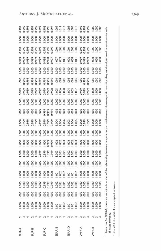
Tabl
e 20
.8C
entr
al,l
ow a
nd h
igh
estim
ates
of
the
rela
tive
risk
of
card
iova
scul
ar d
isea
se (
all a
ges)
for
alte
rnat
ive
clim
ate
scen
ario
s re
lativ
e to
bas
elin
e cl
imat
ea
2000
2001
2005
2010
2020
2030
Subr
egio
nCl
imat
ebM
idLo
w
Hig
hM
idLo
w
Hig
hM
idLo
w
Hig
hM
idLo
w
Hig
hM
idLo
w
Hig
hM
idLo
w
Hig
h
AFR
-D2
1.00
11.
000
1.00
21.
001
1.00
01.
002
1.00
21.
000
1.00
31.
002
1.00
01.
004
1.00
31.
000
1.00
61.
004
1.00
01.
008
31.
001
1.00
01.
003
1.00
11.
000
1.00
31.
002
1.00
01.
004
1.00
31.
000
1.00
51.
004
1.00
01.
008
1.00
51.
000
1.00
94
1.00
21.
000
1.00
41.
002
1.00
01.
004
1.00
31.
000
1.00
51.
004
1.00
01.
007
1.00
51.
000
1.01
11.
007
1.00
01.
013
AFR
-E2
1.00
11.
000
1.00
21.
001
1.00
01.
002
1.00
11.
000
1.00
21.
002
1.00
01.
003
1.00
21.
000
1.00
51.
003
1.00
01.
006
31.
001
1.00
01.
002
1.00
11.
000
1.00
21.
001
1.00
01.
003
1.00
21.
000
1.00
41.
003
1.00
01.
006
1.00
31.
000
1.00
74
1.00
11.
000
1.00
31.
001
1.00
01.
003
1.00
21.
000
1.00
41.
003
1.00
01.
005
1.00
41.
000
1.00
81.
005
1.00
01.
010
AM
R-A
21.
000
1.00
01.
000
1.00
01.
000
1.00
01.
000
1.00
01.
000
1.00
01.
000
0.99
91.
000
1.00
00.
999
1.00
01.
000
0.99
93
1.00
01.
000
1.00
01.
000
1.00
01.
000
1.00
01.
000
1.00
01.
000
1.00
00.
999
1.00
01.
000
0.99
91.
000
1.00
00.
999
41.
000
1.00
01.
000
1.00
01.
000
1.00
01.
000
1.00
01.
000
1.00
01.
000
0.99
91.
000
1.00
00.
999
1.00
01.
000
0.99
9
AM
R-B
21.
001
1.00
01.
001
1.00
11.
000
1.00
11.
001
1.00
01.
002
1.00
11.
000
1.00
21.
002
1.00
01.
003
1.00
21.
000
1.00
43
1.00
11.
000
1.00
11.
001
1.00
01.
002
1.00
11.
000
1.00
21.
001
1.00
01.
003
1.00
21.
000
1.00
41.
003
1.00
01.
005
41.
001
1.00
01.
002
1.00
11.
000
1.00
21.
001
1.00
01.
003
1.00
21.
000
1.00
41.
003
1.00
01.
006
1.00
41.
000
1.00
7
AM
R-D
21.
001
1.00
01.
001
1.00
11.
000
1.00
21.
001
1.00
01.
002
1.00
11.
000
1.00
31.
002
1.00
01.
004
1.00
31.
000
1.00
53
1.00
11.
000
1.00
21.
001
1.00
01.
002
1.00
11.
000
1.00
31.
002
1.00
01.
004
1.00
31.
000
1.00
51.
003
1.00
01.
007
41.
001
1.00
01.
002
1.00
11.
000
1.00
31.
002
1.00
01.
004
1.00
21.
000
1.00
51.
004
1.00
01.
007
1.00
51.
000
1.00
9
EMR
-B2
1.00
01.
000
1.00
11.
001
1.00
01.
001
1.00
11.
000
1.00
11.
001
1.00
01.
002
1.00
11.
000
1.00
31.
002
1.00
01.
004
31.
001
1.00
01.
001
1.00
11.
000
1.00
11.
001
1.00
01.
002
1.00
11.
000
1.00
21.
002
1.00
01.
004
1.00
21.
000
1.00
44
1.00
11.
000
1.00
21.
001
1.00
01.
002
1.00
11.
000
1.00
31.
002
1.00
01.
004
1.00
31.
000
1.00
51.
003
1.00
01.
007
EMR
-D2
1.00
01.
000
1.00
11.
001
1.00
01.
001
1.00
11.
000
1.00
11.
001
1.00
01.
002
1.00
11.
000
1.00
31.
002
1.00
01.
004
31.
001
1.00
01.
001
1.00
11.
000
1.00
11.
001
1.00
01.
002
1.00
11.
000
1.00
21.
002
1.00
01.
004
1.00
21.
000
1.00
54
1.00
11.
000
1.00
21.
001
1.00
01.
002
1.00
11.
000
1.00
31.
002
1.00
01.
004
1.00
31.
000
1.00
51.
003
1.00
01.
007
Anthony J. McMichael et al. 1569
EUR
-A2
1.00
01.
000
1.00
01.
000
1.00
01.
000
1.00
01.
000
1.00
01.
000
1.00
00.
999
1.00
01.
000
0.99
90.
999
1.00
00.
999
31.
000
1.00
01.
000
1.00
01.
000
1.00
01.
000
1.00
00.
999
1.00
01.
000
0.99
90.
999
1.00
00.
999
0.99
91.
000
0.99
94
1.00
01.
000
1.00
01.
000
1.00
01.
000
1.00
01.
000
0.99
91.
000
1.00
00.
999
0.99
91.
000
0.99
90.
999
1.00
00.
999
EUR
-B2
1.00
01.
000
1.00
01.
000
1.00
01.
000
1.00
01.
000
0.99
91.
000
1.00
00.
999
0.99
91.
000
0.99
90.
999
1.00
00.
999
31.
000
1.00
01.
000
1.00
01.
000
1.00
01.
000
1.00
00.
999
1.00
01.
000
0.99
90.
999
1.00
00.
999
0.99
91.
000
0.99
94
1.00
01.
000
1.00
01.
000
1.00
00.
999
1.00
01.
000
0.99
91.
000
1.00
00.
999
0.99
91.
000
0.99
90.
999
1.00
00.
998
EUR
-C2
1.00
01.
000
0.99
91.
000
1.00
00.
999
1.00
01.
000
0.99
90.
999
1.00
00.
999
0.99
91.
000
0.99
80.
999
1.00
00.
998
31.
000
1.00
00.
999
1.00
01.
000
0.99
90.
999
1.00
00.
999
0.99
91.
000
0.99
90.
999
1.00
00.
998
0.99
91.
000
0.99
84
1.00
01.
000
0.99
91.
000
1.00
00.
999
0.99
91.
000
0.99
90.
999
1.00
00.
998
0.99
91.
000
0.99
70.
998
1.00
00.
997
SEA
R-B
21.
001
1.00
01.
002
1.00
11.
000
1.00
31.
002
1.00
01.
004
1.00
21.
000
1.00
51.
004
1.00
01.
007
1.00
41.
000
1.00
93
1.00
11.
000
1.00
31.
002
1.00
01.
003
1.00
21.
000
1.00
41.
003
1.00
01.
006
1.00
41.
000
1.00
91.
005
1.00
01.
011
41.
002
1.00
01.
004
1.00
21.
000
1.00
41.
003
1.00
01.
006
1.00
41.
000
1.00
81.
006
1.00
01.
011
1.00
71.
000
1.01
4
SEA
R-D
21.
001
1.00
01.
002
1.00
11.
000
1.00
21.
002
1.00
01.
003
1.00
21.
000
1.00
41.
003
1.00
01.
006
1.00
41.
000
1.00
83
1.00
11.
000
1.00
31.
001
1.00
01.
003
1.00
21.
000
1.00
41.
003
1.00
01.
005
1.00
41.
000
1.00
81.
005
1.00
01.
009
41.
002
1.00
01.
004
1.00
21.
000
1.00
41.
003
1.00
01.
005
1.00
41.
000
1.00
71.
005
1.00
01.
011
1.00
71.
000
1.01
3
WPR
-A2
1.00
01.
000
1.00
01.
000
1.00
01.
000
1.00
01.
000
1.00
01.
000
1.00
00.
999
1.00
01.
000
0.99
90.
999
1.00
00.
999
31.
000
1.00
01.
000
1.00
01.
000
1.00
01.
000
1.00
00.
999
1.00
01.
000
0.99
90.
999
1.00
00.
999
0.99
91.
000
0.99
94
1.00
01.
000
1.00
01.
000
1.00
01.
000
1.00
01.
000
0.99
91.
000
1.00
00.
999
0.99
91.
000
0.99
90.
999
1.00
00.
999
WPR
-B2
1.00
01.
000
1.00
01.
000
1.00
01.
000
1.00
01.
000
1.00
01.
000
1.00
01.
000
1.00
01.
000
1.00
01.
000
1.00
01.
000
31.
000
1.00
01.
000
1.00
01.
000
1.00
01.
000
1.00
01.
000
1.00
01.
000
1.00
01.
000
1.00
01.
000
1.00
01.
000
1.00
04
1.00
01.
000
1.00
01.
000
1.00
01.
000
1.00
01.
000
1.00
01.
000
1.00
01.
000
1.00
01.
000
1.00
01.
000
1.00
01.
000
aN
ote
that
for
SEA
R-B
,the
re a
re n
o su
itabl
e st
udie
s of
the
rel
atio
nshi
p be
twee
n te
mpe
ratu
re a
nd c
ardi
ovas
cula
r di
seas
e-sp
ecifi
c m
orta
lity;
they
are
the
refo
re b
ased
on
rela
tions
hips
with
all-c
ause
mor
talit
y.b
2 =
s550
,3 =
s750
,4 =
unm
itiga
ted
emis
sion
s.

estimate assumes complete adaptation to a changing climate, and there-fore no change in the relative risk as the climate changes.
There is therefore a need for further time-series studies, applying astandard approach to populations living in as wide a range of climatesas possible. Previous analyses have focused mainly on temperate zones,where the winter effects are greatest, potentially causing over-estimationof the reduced burden attributable to climate change (e.g. Martens1998a). More analyses of temperature–mortality relationships are there-fore required in tropical developing countries.
Such studies should attempt to estimate formally the degree to whichadaptation may decrease mortality, and to which observed associationsbetween climate and mortality reflect displaced rather than additionaldeaths. Finally, there is a need for greater investigation of the healthburden of morbidity associated with temperature extremes, including,for example, inability to work in extreme temperatures.
3.7 Diarrhoeal disease
Diarrhoeal diseases are highly sensitive to climate, showing seasonal variations in numerous sites (Drasar et al. 1978). This observation is sup-ported by regression analyses of the effects of seasonal and longer-termvariation in a limited number of sites (Checkley et al. 2000; Singh et al.2001). The results of a literature search on the associations between diar-rhoeal disease and climate are shown in Appendix B, Table B.2. Theclimate-sensitivity of diarrhoeal disease is consistent with observationsof the direct effects of climate variables on the causative agents. Tem-perature and relative humidity have a direct influence on the rate of repli-cation of bacterial and protozoan pathogens, and on the survival ofenteroviruses in the environment (Blaser et al. 1995). Rainfall may affectthe frequency and level of contamination of drinking water (Curriero et al. 2001).
Quantitative relationships can be defined between climate variationsand incidence, which can in turn be directly linked to the outputs ofglobal climate change models. There are, however, challenges and uncer-tainties in estimating the magnitude of effects.
• The sites from which these relationships were defined cover only asmall part of the spectrum of global climate variation. Different rela-tionships may apply at higher or lower temperatures.
• The relative importance of different pathogens and modes of transmission (e.g. via water, food, insects or human–human contact)varies between locations, and is heavily influenced by level of sanita-tion (Black and Lanata 1995). As the pathogens are known to varyin their response to climate (e.g. Cook et al. 1990; Chaudhury et al.1996), this will cause uncertainty in extrapolating temperature rela-tionships from local studies to other regions with different levels ofdevelopment.
1570 Comparative Quantification of Health Risks

• Pathogens vary in the severity of clinical symptoms, and the likeli-hood that they will be reported to health services (e.g. Wheeler et al.1999). Therefore, climate–disease relationships derived only frompassive reporting may differ from those based on other methods ofsurveillance.
• While several studies describe climate effects on particular diarrhoeapathogens (e.g. Eberhard et al. 1999; Konno et al. 1983; Purohit et al. 1998), these cannot be used directly to estimate effects on diar-rhoeal disease without information on: (i) their relative contributionto overall disease incidence, and (ii) equivalent data on climate sensi-tivity and relative prevalence for all other diarrhoea pathogens.
• Despite convincing evidence on the effect of extreme rainfall on water-borne outbreaks of diarrhoea, even in highly developed countries(Curriero et al. 2001), this cannot easily be generalized to the totalburden of diarrhoeal disease without information on the relative con-tribution of such outbreaks to overall diarrhoea incidence.
• Rainfall effects on overall diarrhoea (where observed) are non-linear,and cannot easily be extrapolated to other regions.
In order to minimize these uncertainties, we restricted our estimatesto the effect of increasing temperatures on the incidence of all-cause diar-rhoea reported to health services (i.e. without attempting to make sepa-rate estimates for different pathogens, transmission routes, severities, orfor the more complex associations with rainfall). There are importantresidual uncertainties related to the extrapolation of temperature rela-tionships from specific study sites to others with different temperatureregimes and levels of development, and climate effects on reported diar-rhoea compared to the true burden of disease. Projections of increasingfrequency of extreme wet seasons are very large (e.g. two to five timesincrease in the regions analysed; Palmer and Ralsanen 2002), andextreme precipitation is associated with increased diarrhoea in bothdeveloped (Curriero et al. 2001) and developing (Singh et al. 2001) countries.
Graded maps of 3.75 ∞ longitude by 2.5 ∞ latitude resolution showingthe change in temperature under the alternative scenarios were overlaidwith 0.5 ∞¥0.5 ∞ resolution maps of predicted population distributionsfor the 2020s and 2050s in a GIS. The GIS was used to calculate theaverage change in exposure (temperature) for each population grid-cell.
Although seasonality of diarrhoeal disease is well recognized, thequantitative relationship between climate and overall diarrhoea inci-dence has only been explicitly measured in two studies. Both studiesdescribed relationships with all-cause diarrhoea, that is, specificpathogens were not differentiated. Checkley et al. (2000) used time-seriesanalysis to correlate measurements of temperature and relative humid-ity against daily hospital admissions at a single paediatric diarrhoeal
Anthony J. McMichael et al. 1571

disease clinic in Lima, Peru (Figure 20.4) for just under 6 years. A totalof 57331 admissions were recorded during the study. The analysisshowed a 4% (95% CI 2–5%) increase in admissions for each degreecentigrade increase in temperature during the hotter months, and a 12%(95% CI 10–14%) per degree centigrade increase in the cooler months,averaging at an 8% (95% CI 7–9%) per degree centigrade increase overthe course of the study. During the 1997–1998 El Niño period there was an additional increase in admissions above that expected on the basisof pre-El Niño temperature relationships, but no association with rela-tive humidity independent of temperature. No rainfall during thatperiod.
In the Checkley et al. study, exposure (climate) data were recorded atlocal meteorological stations, and can be considered to have negligiblemeasurement error at the population level. The analysis independentlycontrolled for seasonal variations and long-term trends, imparting highconfidence to the observed effect of temperature on the outcomerecorded. The positive correlation with temperature is also biologicallyplausible, as a high proportion of diarrhoea cases in many tropical devel-oping countries are caused by bacteria, entamoeba and protozoa (Black
1572 Comparative Quantification of Health Risks
Figure 20.4 Hospitalizations for diarrhoea (upper line) correspond closelywith temperature (lower line) at a clinic in Lima, Peru
Note: Shaded region corresponds to the 1997–1998 El Niño event.
Source: Checkley et al. (2000).
80
60
40
20
0
26
24
23
20
18
16
14
Adm
issi
ons
for
diar
rhoe
aT
empe
ratu
re (
°C)

and Lanata 1995), which are favoured by high temperatures. The prin-ciple limitations of the study by Checkley et al. are that the outcomerecorded may not be representative of climate effects on: (i) less severedisease (i.e. not requiring hospitalization) or more severe disease (diar-rhoeal deaths), or (ii) disease in adults rather than children.
Singh et al. (2001) used similar time-series analyses to correlatemonthly reported incidence of diarrhoea throughout Fiji against varia-tions in temperature and rainfall, after allowing for the effects of sea-sonal variation and long-term trend. The study covered the periodbetween 1978 and 1998, with an average of some 1000 reported casesfor each of the 228 study months. Reported incidence increased byapproximately 3% (95% CI 1.2–5.0%) for each degree centigradeincrease in temperature, by 2% (95% CI 1.5–2.3%) per unit increase inrainfall above average rainfall conditions (5¥10–5 kg/m2 per min), andby 8% per unit decrease below average conditions. The pattern is sup-ported by a positive geographical correlation between temperature andincidence in 18 Pacific Island countries (Singh et al. 2001). Climate mea-surements were from a 2.5 ∞¥2.5 ∞ cell of a global gridded data set cor-responding to Fiji. The use of monthly averages of climate data from thislarge geographical area may not have reflected the full range of climateexposures of the population; this would have introduced random errorand decreased sensitivity. Low rainfall may force use of contaminatedwater, while high rainfall may contaminate water through flooding. Themajor limitations of this study are lack of a clear clinical or laboratorydefinition for diarrhoea, and lack of information on the age distributionof cases.
We are not aware of any similar studies of climate effects on all-causediarrhoea in developed regions, although studies have been carried outon some subsets of total incidence. Bentham (1997) showed that the incidence of food poisoning, usually caused by bacteria, increased byapproximately 9% per degree centigrade in England and Wales. Konnoet al. (1983) demonstrated a non-linear inverse relationship betweenrotavirus infection and temperature in Japan. The relative importance ofpathogens that thrive at lower temperatures appears to be greater in pop-ulations with higher standards of living, who have access to clean waterand sanitation and for whom there is no clear and consistent evidencefor peaks in all-cause diarrhoea in warmer months. This is in contrastto the situation of less well-off populations, where diarrhoea is usuallymore common in warmer, wetter months, as well demonstrated by clearsummer peaks of diarrhoea in black, but not white, infants in Johan-nesburg during the 1970s (Robins-Browne 1984).
For this assessment we defined developing countries as those with percapita incomes lower than the richer of the two study countries (Fiji) inthe year 2000—approximately US$6000/year in 1990 US dollars. Forsuch countries, we applied a dose–response relationship of 5% increasein diarrhoea incidence per degree centigrade increase in temperature, to
Anthony J. McMichael et al. 1573
both sexes and all age groups. This is consistent with the relationshipsderived from the two studies described above. We chose 5% rather thanthe arithmetic mean of the constants from the two studies (5.5%) fortwo reasons: (i) to avoid giving a false impression of precision based ononly two estimates, each with their own confidence intervals, and (ii) inorder to be conservative.
Although the confidence intervals around the estimates from the indi-vidual studies are relatively small, these clearly cover only a small rangeof climatic and socioeconomic environments. As described above, Check-ley et al. (2000) showed that even in a single socioeconomic setting thetemperature dependence of diarrhoeal disease may vary across the tem-perature range or, less plausibly, with non-climatic seasonal variations.This introduces uncertainty when extrapolating such a single relation-ship. There is also potential bias: if the temperature-responsiveness isindeed greater at low temperatures, extrapolation of an average valuewill tend to underestimate effects in areas that are on average colder, andoverestimate in hotter regions. However, the average annual tempera-tures experienced by the residents of the areas to which we extrapolatedthis relationship was 20.3 ∞C, as calculated by averaging the tempera-tures in each 1 ∞¥1 ∞grid-cell weighted by the population. This is in themid-range of the temperatures experienced throughout the year in Lima(16–26 ∞C), and cooler than those in the capital of Fiji (23–27 ∞C) (WorldClimate 2002). Our extrapolation tended towards being conservative,but with significant uncertainty. Therefore, we place a wide uncertaintyrange (0–10%) on this value.
As there are no such studies published for developed regions, we madethe assumption that overall diarrhoea incidence in richer countries isinsensitive to climate change, that is, 0% (-5 to +5%) change per degreecentigrade temperature change. Relative risks for each country undereach scenario were calculated by multiplying the projected increase intemperature by the relevant exposure–response value. The quoted esti-mate for each subregion is the population-weighted average of the rela-tive risks for each country in the subregion (Table 20.9). In addition tochanges in baseline diarrhoeal disease over time, we assumed that theclimate sensitivity of diarrhoea in developing countries will decrease asthey become better off. For projections of relative risks for years after2000, we used projections of future changes in GDP (WHO/EIP/GPE,unpublished data, 2000) to apply the relationship used above—that is,overall diarrhoea incidence does not respond to temperature in anycountry that attains a per capita GDP of at least US$6000/year. Relativerisks for each time point were then calculated as above.
The quantitative estimates in this analysis were highly sensitive to the exposure–response relationship, around which there is substantialuncertainty due to the very small number of analysed time-series. The estimates could be rapidly improved by analysis of climate exposure–response relationships from sites from a wider climatic and
1574 Comparative Quantification of Health Risks

Anthony J. McMichael et al. 1575
Tabl
e 20
.9C
entr
al,l
ow a
nd h
igh
estim
ates
of
the
rela
tive
risk
of
diar
rhoe
a fo
r al
tern
ativ
e cl
imat
e sc
enar
ios
rela
tive
to
base
line
clim
ate
2000
2001
2005
2010
2020
2030
Subr
egio
nCl
imat
eaM
idLo
w
Hig
hM
idLo
w
Hig
hM
idLo
w
Hig
hM
idLo
w
Hig
hM
idLo
w
Hig
hM
idLo
wH
igh
AFR
-D2
1.01
1.00
1.03
1.02
1.00
1.03
1.02
1.00
1.04
1.03
1.00
1.06
1.04
1.00
1.08
1.05
0.99
1.10
31.
021.
001.
041.
021.
001.
041.
031.
001.
051.
041.
001.
071.
051.
001.
111.
060.
991.
134
1.02
1.00
1.05
1.02
1.00
1.05
1.03
1.00
1.07
1.05
1.00
1.09
1.07
1.00
1.14
1.08
0.99
1.16
AFR
-E2
1.01
1.00
1.03
1.02
1.00
1.03
1.02
1.00
1.04
1.03
1.00
1.06
1.04
0.99
1.08
1.05
0.99
1.11
31.
021.
001.
041.
021.
001.
041.
021.
001.
051.
031.
001.
071.
050.
991.
101.
060.
991.
134
1.02
1.00
1.05
1.03
1.00
1.05
1.03
1.00
1.07
1.04
0.99
1.09
1.06
0.99
1.13
1.08
0.99
1.16
AM
R-A
21.
000.
991.
021.
000.
981.
021.
000.
981.
021.
000.
971.
031.
000.
961.
051.
000.
951.
063
1.00
0.99
1.02
1.00
0.98
1.02
1.00
0.98
1.02
1.00
0.97
1.03
1.00
0.96
1.05
1.00
0.94
1.06
41.
000.
981.
021.
000.
981.
021.
000.
971.
031.
000.
961.
041.
000.
941.
061.
000.
931.
08
AM
R-B
21.
000.
991.
021.
000.
991.
021.
000.
981.
021.
000.
971.
031.
000.
961.
041.
000.
951.
053
1.00
0.99
1.02
1.00
0.99
1.02
1.00
0.98
1.02
1.00
0.97
1.03
1.00
0.96
1.05
1.00
0.94
1.06
41.
000.
981.
021.
000.
981.
031.
000.
971.
031.
000.
961.
041.
000.
941.
061.
000.
921.
08
AM
R-D
21.
011.
001.
031.
011.
001.
031.
021.
001.
041.
031.
001.
051.
020.
981.
061.
020.
961.
073
1.02
1.00
1.03
1.02
1.00
1.03
1.02
1.00
1.05
1.03
1.00
1.06
1.02
0.97
1.07
1.02
0.96
1.08
41.
021.
001.
041.
021.
001.
051.
031.
001.
061.
041.
001.
081.
030.
971.
091.
020.
951.
10
EMR
-B2
1.01
1.00
1.03
1.01
1.00
1.03
1.02
0.99
1.04
1.02
0.99
1.06
1.00
0.95
1.05
1.00
0.94
1.06
31.
011.
001.
031.
011.
001.
031.
020.
991.
041.
020.
991.
051.
000.
951.
051.
000.
941.
064
1.02
0.99
1.04
1.02
0.99
1.05
1.03
0.99
1.06
1.04
0.99
1.08
1.00
0.93
1.08
1.00
0.91
1.09
EMR
-D2
1.02
1.00
1.03
1.02
1.00
1.04
1.02
1.00
1.05
1.03
1.00
1.06
1.05
1.00
1.10
1.06
1.00
1.12
31.
021.
001.
031.
021.
001.
041.
031.
001.
051.
031.
001.
071.
051.
001.
101.
061.
001.
134
1.03
1.00
1.05
1.03
1.00
1.06
1.04
1.00
1.08
1.05
1.00
1.10
1.08
1.00
1.15
1.09
1.00
1.19
cont
inue
d

1576 Comparative Quantification of Health Risks
Tabl
e 20
.9C
entr
al,l
ow a
nd h
igh
estim
ates
of
the
rela
tive
risk
of
diar
rhoe
a fo
r al
tern
ativ
e cl
imat
e sc
enar
ios
rela
tive
to b
asel
ine
clim
ate
(con
tinue
d)
2000
2001
2005
2010
2020
2030
Subr
egio
nCl
imat
eM
idLo
w
Hig
hM
idLo
w
Hig
hM
idLo
w
Hig
hM
idLo
w
Hig
hM
idLo
w
Hig
hM
idLo
wH
igh
EUR
-A2
1.00
0.98
1.02
1.00
0.98
1.02
1.00
0.98
1.02
1.00
0.97
1.03
1.00
0.95
1.05
1.00
0.94
1.06
31.
000.
981.
021.
000.
981.
021.
000.
971.
031.
000.
971.
031.
000.
951.
051.
000.
941.
064
1.00
0.98
1.02
1.00
0.98
1.02
1.00
0.97
1.03
1.00
0.96
1.04
1.00
0.94
1.06
1.00
0.92
1.08
EUR
-B2
1.01
0.99
1.03
1.01
0.99
1.03
1.01
0.99
1.04
1.02
0.98
1.05
1.02
0.97
1.07
1.01
0.94
1.07
31.
010.
991.
031.
010.
991.
031.
010.
991.
041.
020.
981.
051.
020.
971.
071.
010.
941.
084
1.01
0.99
1.03
1.01
0.99
1.04
1.02
0.98
1.05
1.02
0.98
1.06
1.02
0.96
1.09
1.01
0.93
1.09
EUR
-C2
1.02
1.00
1.03
1.02
1.00
1.04
1.01
0.98
1.03
1.01
0.98
1.04
1.01
0.96
1.06
1.00
0.94
1.07
31.
021.
001.
031.
021.
001.
041.
010.
981.
031.
010.
981.
041.
010.
961.
061.
000.
941.
074
1.02
1.00
1.04
1.02
1.00
1.05
1.01
0.98
1.04
1.01
0.97
1.06
1.01
0.95
1.08
1.00
0.92
1.08
SEA
R-B
21.
011.
001.
021.
011.
001.
021.
011.
001.
031.
000.
981.
031.
000.
971.
041.
000.
951.
053
1.01
1.00
1.03
1.01
1.00
1.03
1.02
0.99
1.04
1.00
0.97
1.04
1.00
0.95
1.05
1.00
0.94
1.06
41.
021.
001.
041.
021.
001.
041.
020.
991.
051.
000.
961.
041.
000.
941.
071.
000.
921.
08
SEA
R-D
21.
021.
001.
031.
021.
001.
041.
031.
001.
051.
031.
001.
071.
051.
001.
101.
061.
001.
133
1.02
1.00
1.04
1.02
1.00
1.04
1.03
1.00
1.06
1.04
1.00
1.08
1.06
1.00
1.12
1.07
1.00
1.15
41.
031.
001.
051.
031.
001.
061.
041.
001.
081.
051.
001.
101.
071.
001.
151.
091.
001.
19
WPR
-A2
1.00
0.99
1.01
1.00
0.99
1.01
1.00
0.98
1.02
1.00
0.97
1.03
1.00
0.96
1.04
1.00
0.95
1.05
31.
000.
991.
011.
000.
991.
011.
000.
981.
021.
000.
981.
021.
000.
961.
041.
000.
951.
054
1.00
0.98
1.02
1.00
0.98
1.02
1.00
0.97
1.03
1.00
0.96
1.04
1.00
0.94
1.06
1.00
0.93
1.07
WPR
-B2
1.01
1.00
1.03
1.01
1.00
1.03
1.02
1.00
1.04
1.03
1.00
1.06
1.00
0.96
1.05
1.00
0.95
1.06
31.
011.
001.
031.
011.
001.
031.
021.
001.
041.
031.
001.
061.
000.
961.
051.
000.
951.
064
1.02
1.00
1.05
1.03
1.00
1.05
1.03
1.00
1.07
1.05
1.00
1.09
1.00
0.93
1.08
1.01
0.92
1.09
a2
=s5
50,3
=s7
50,4
=un
miti
gate
d em
issi
ons.

socioeconomic spectrum. Future studies should also explicitly measurethe degree to which economic development and improved levels of sanitation influence vulnerability to the effects of climate variation ondiarrhoeal disease.
3.8 Malnutrition
Multiple biological and social factors affect the incidence of malnutri-tion, but one of the fundamental determinants is the availability of staplefoods. Climate change may affect this through the balance of the(broadly negative) effects of changes in temperature and precipitation,and (broadly positive) effects of higher CO2 levels on yields of majorfood crops (e.g. IPCC 1996; Rosenzweig and Parry 1994; see also Appendix B, Table B.4). These effects are likely to vary markedly withgeography: productivity is projected to increase in higher-latitude pro-ducers such as Canada and the United States, but to decrease closer tothe equator. The global food trade system may be able to absorb theseeffects at the global level. However, climate change can be expected to have significant effects on food poverty in some regions, owing to variation in both productivity and in economic capacity to cope (Parryet al. 1999).
Crop models have been validated at 124 sites in 18 countries over a wide range of environments (e.g. Otter-Nacke et al. 1986). However,estimation of changes in food availability (and by inference malnutri-tion) requires additional analyses of the geographical variation in effectson food production, and of food trade patterns. Only one modellinggroup (Parry et al. 1999) has integrated a basic physiological model of climate change effects on region-specific crop production with foodtrade models, in order to make projections of the numbers of peopleactually at risk of hunger. All results presented here were based on the model described in Parry et al. (1999) and other work by the samegroup.
As for other potential effects of climate change, there is considerableuncertainty over the degree to which current relationships, such as thosebetween climate and crops, and food trade systems will remain constantover time. The most important uncertainties probably relate to the abilityof the world food trade system to adapt to changes in production (Dyson1999; Waterlow et al. 1998). Although these are the most completemodels currently available, they do not describe the likely effect ofclimate change on more complex pathways, such as animal husbandry,or the relative importance of fruit and vegetable production. These inturn may affect micronutrient (e.g. vitamin A, iodine, iron and zinc) deficiency.
Global distribution of temperature, rainfall and CO2 were mapped for each of the alternative scenarios, as described above. Climatedose–response relationships have been defined for yields of major graincereals and soybean, which account for 85% of world cereal exports.
Anthony J. McMichael et al. 1577

Effects of temperature and precipitation, and the beneficial effects ofhigher CO2 levels, have been defined using the IBSNAT-ICASA dynamiccrop growth models (IBSNAT 1989). The exposure distributionsdescribed above were applied to these crop growth models, and thederived yield functions were extrapolated to other crops and regions onthe basis of agro-climatic similarity.
These crop yield estimates are used as inputs for the Basic LinkedSystem world food trade model. This consists of a linked series of 40national and regional food models, representing food production, theeffects of market forces and government policies on prices and trade, andtrends in agricultural, economic and technological conditions over time(see Fischer et al. 1988 for a full description).
The model is represented schematically in Figure 20.5. Principal characteristics of this model are:
• no major changes in the political or economic context of world foodtrade or in food production technology;
• population growth to occur following the World Bank mid-range estimate (World Bank 1994) i.e. 10.7 billion by the 2080s;
• GDP to accumulate as projected by EMF14 (Energy Modeling Forum1995);
• a 50% trade liberalization in agriculture is introduced gradually by2020.
The model results in an estimation of national food availability. Thisis used to generate an estimate of per capita food availability in eachcountry, assuming that this food is distributed among the population following a skewed (beta) distribution. The final model output is thenumber or proportion of the population in each subregion who do nothave access to sufficient food to maintain a basal metabolic rate of 1.4,which is the Food and Agriculture Organization of the United Nations’(FAO) definition of undernourishment (FAO 1987).
The model generates outputs for continents made up principally ofvulnerable developing countries (thus excluding China and the formerSoviet Union, countries in North America, and in western and easternEurope). As these model continents do not map directly on to the sub-regions, we generated estimates for each subregion by calculating theproportion of the population that lives within each continent in the foodavailability model. Where more than 90% of the subregion populationlive within a single model continent, we quoted the model estimate forthat continent. Otherwise an average was calculated, weighted by thedistribution of the subregion population among the various continents.While the subregions mapped reasonably well on to the climatechange/food availability model continents, the aggregation meant thatsome of the geographical variation in vulnerability was lost. Mostnotably, despite severe problems in some countries, EUR-C was assumed
1578 Comparative Quantification of Health Risks

Anthony J. McMichael et al. 1579
Figure 20.5 Key elements of the crop yields and world food trade study
ET Evapotranspiration.
Source: Rosenzweig et al. (1993).
Climate change scenarios
Crop models: wheat, rice, maize, soybean
Crop yield by site and scenario
ET, irrigation, season length
Aggregation of site results
Agro-ecological zone analysis
Yield functions byregion
Yield = f (T, P, CO2)
Yield change estimates commodity group and
country/region
World food trade model
Economic consequencesShifts in trade
Incidence of food poverty
Technology projections
Economicgrowth rates
Adaptations
Population trends
Greenhouse policies
GCMsTrace gases
Observed climate
CO2 effects Farm level adaptations
Sensitivity tests
1580 Comparative Quantification of Health Risks
not to suffer from malnutrition as it lies within the “developed” Euro-pean continent of the food availability model.
Preliminary analysis correlating estimates for the 1990s at the level ofthe model regions (data not shown) indicated that the model output waspositively related to more direct measures of malnutrition, such as theincidence of underweight, and stunting and wasting in children aged <5years, as measured by the WHO Global Database on Child Growth andMalnutrition (WHO 2002). The aggregation of the food availabilitymodel means that this correlation was based on only a small number ofindependent data points. We therefore did not attempt to make anyquantitative estimate of these relationships. Instead, the relative risk ofthe incidence of energy shortfall (Table 20.10) was interpreted as beingdirectly proportional to the relative risk of suffering from the risk factor“underweight”. The relative risk estimates were therefore applied to alldiseases affected by the underweight risk factor (see chapter 2). Theseinclude diarrhoea and malaria. We therefore assumed that these diseasesare affected in two distinct ways by climate change—through meteoro-logical effects on the pathogens and vectors, and through increased sus-ceptibility of the human population due to undernutrition.
In common with most climate change impact assessments, the pub-lished studies do not quote uncertainties around the various relationshipsin the model, either separately or aggregated. Small variations in theinitial conditions of a single climate model (the HadCM2 ensemble) gen-erated only slight variations in projections of crop production and inci-dence of food shortfall. Using a different climate model (HadCM3),however, generated markedly different projections (Parry et al. 1999).These comparisons relate to only part of the possible error, as they donot address uncertainties in the trade and social components of themodel.
From the published descriptions of the model, there is no reason toassume that the estimates generated were systematically biased eitherupward or downward. In the absence of formal sensitivity analyses ofthe complete model, however, uncertainty estimates are arbitrary. Wepresented the relative risks generated above as mid-range estimates, withthe upper and lower range covering a complete adaptation to anychanges in agricultural output (i.e. no change in risk), to a doubling ofthe estimate of the relative risk calculated above. However, this uncer-tainty range should be treated with caution. Priorities for the future areinvestigations of:
• variation in output when using a wider range of food productionmodels as inputs to the food trade/availability models;
• sensitivity of estimates to the various climate scenarios;
• sensitivity analyses to estimate uncertainty around the exposure–response relationships;

Anthony J. McMichael et al. 1581
Tabl
e 20
.10
Cen
tral
,low
and
hig
h es
timat
es o
f th
e re
lativ
e ri
sk o
f m
alnu
triti
on fo
r al
tern
ativ
e cl
imat
e sc
enar
ios
rela
tive
toba
selin
e cl
imat
e
2000
2001
2005
2010
2020
2030
Subr
egio
nCl
imat
eaM
idLo
w
Hig
hM
idLo
w
Hig
hM
idLo
w
Hig
hM
idLo
w
Hig
hM
idLo
w
Hig
hM
idLo
w
Hig
h
AFR
-D2
1.01
1.00
1.02
1.01
1.00
1.02
1.01
1.00
1.03
1.02
1.00
1.04
1.03
1.00
1.06
1.03
1.00
1.06
31.
011.
001.
031.
011.
001.
031.
021.
001.
041.
031.
001.
051.
041.
001.
081.
041.
001.
094
1.01
1.00
1.01
1.01
1.00
1.01
1.01
1.00
1.02
1.01
1.00
1.03
1.02
1.00
1.04
1.02
1.00
1.04
AFR
-E2
1.01
1.00
1.02
1.01
1.00
1.02
1.01
1.00
1.03
1.02
1.00
1.04
1.03
1.00
1.06
1.03
1.00
1.06
31.
011.
001.
021.
011.
001.
031.
021.
001.
041.
021.
001.
051.
041.
001.
071.
041.
001.
084
1.01
1.00
1.01
1.01
1.00
1.02
1.01
1.00
1.02
1.01
1.00
1.03
1.02
1.00
1.04
1.02
1.00
1.05
AM
R-A
21.
001.
001.
001.
001.
001.
001.
001.
001.
001.
001.
001.
001.
001.
001.
001.
001.
001.
003
1.00
1.00
1.00
1.00
1.00
1.00
1.00
1.00
1.00
1.00
1.00
1.00
1.00
1.00
1.00
1.00
1.00
1.00
41.
001.
001.
001.
001.
001.
001.
001.
001.
001.
001.
001.
001.
001.
001.
001.
001.
001.
00
AM
R-B
21.
021.
001.
031.
021.
001.
031.
021.
001.
051.
031.
001.
061.
051.
001.
091.
051.
001.
103
1.03
1.00
1.07
1.04
1.00
1.07
1.05
1.00
1.10
1.07
1.00
1.13
1.10
1.00
1.20
1.11
1.00
1.22
41.
001.
001.
001.
001.
001.
001.
001.
001.
001.
001.
001.
001.
001.
001.
011.
001.
001.
00
AM
R-D
21.
021.
001.
031.
021.
001.
031.
021.
001.
051.
031.
001.
061.
051.
001.
091.
051.
001.
103
1.03
1.00
1.07
1.04
1.00
1.07
1.05
1.00
1.10
1.07
1.00
1.13
1.10
1.00
1.20
1.11
1.00
1.22
41.
001.
001.
001.
001.
001.
001.
001.
001.
001.
001.
001.
001.
001.
001.
011.
001.
001.
00
EMR
-B2
1.01
1.00
1.02
1.01
1.00
1.02
1.01
1.00
1.03
1.02
1.00
1.04
1.03
1.00
1.06
1.03
1.00
1.06
31.
021.
001.
041.
021.
001.
041.
031.
001.
061.
041.
001.
081.
061.
001.
121.
061.
001.
134
1.00
1.00
1.00
1.00
1.00
1.00
1.00
1.00
1.00
1.00
1.00
1.00
1.00
1.00
1.01
1.00
1.00
1.00
EMR
-D2
1.02
1.00
1.04
1.02
1.00
1.05
1.03
1.00
1.07
1.04
1.00
1.09
1.07
1.00
1.13
1.07
1.00
1.15
31.
031.
001.
071.
041.
001.
071.
051.
001.
101.
071.
001.
131.
101.
001.
201.
111.
001.
224
1.02
1.00
1.05
1.03
1.00
1.05
1.04
1.00
1.07
1.05
1.00
1.10
1.07
1.00
1.15
1.08
1.00
1.16
cont
inue
d
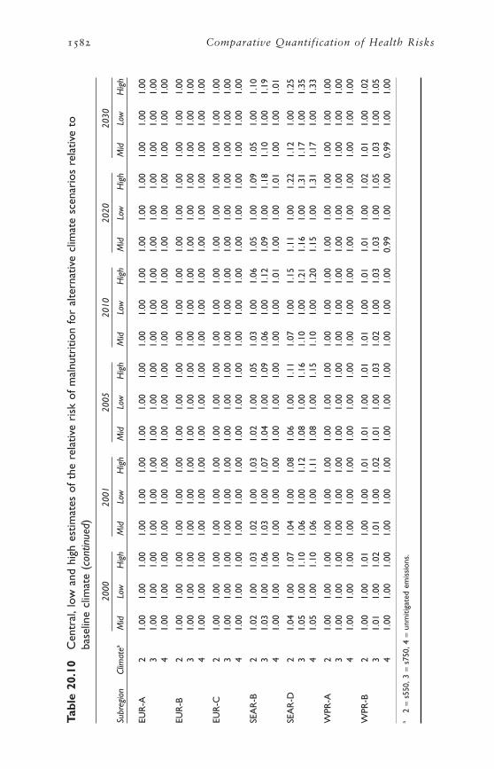
1582 Comparative Quantification of Health Risks
Tabl
e 20
.10
Cen
tral
,low
and
hig
h es
timat
es o
f th
e re
lativ
e ri
sk o
f m
alnu
triti
on fo
r al
tern
ativ
e cl
imat
e sc
enar
ios
rela
tive
toba
selin
e cl
imat
e (c
ontin
ued)
2000
2001
2005
2010
2020
2030
Subr
egio
nCl
imat
eaM
idLo
w
Hig
hM
idLo
w
Hig
hM
idLo
w
Hig
hM
idLo
w
Hig
hM
idLo
w
Hig
hM
idLo
w
Hig
h
EUR
-A2
1.00
1.00
1.00
1.00
1.00
1.00
1.00
1.00
1.00
1.00
1.00
1.00
1.00
1.00
1.00
1.00
1.00
1.00
31.
001.
001.
001.
001.
001.
001.
001.
001.
001.
001.
001.
001.
001.
001.
001.
001.
001.
004
1.00
1.00
1.00
1.00
1.00
1.00
1.00
1.00
1.00
1.00
1.00
1.00
1.00
1.00
1.00
1.00
1.00
1.00
EUR
-B2
1.00
1.00
1.00
1.00
1.00
1.00
1.00
1.00
1.00
1.00
1.00
1.00
1.00
1.00
1.00
1.00
1.00
1.00
31.
001.
001.
001.
001.
001.
001.
001.
001.
001.
001.
001.
001.
001.
001.
001.
001.
001.
004
1.00
1.00
1.00
1.00
1.00
1.00
1.00
1.00
1.00
1.00
1.00
1.00
1.00
1.00
1.00
1.00
1.00
1.00
EUR
-C2
1.00
1.00
1.00
1.00
1.00
1.00
1.00
1.00
1.00
1.00
1.00
1.00
1.00
1.00
1.00
1.00
1.00
1.00
31.
001.
001.
001.
001.
001.
001.
001.
001.
001.
001.
001.
001.
001.
001.
001.
001.
001.
004
1.00
1.00
1.00
1.00
1.00
1.00
1.00
1.00
1.00
1.00
1.00
1.00
1.00
1.00
1.00
1.00
1.00
1.00
SEA
R-B
21.
021.
001.
031.
021.
001.
031.
021.
001.
051.
031.
001.
061.
051.
001.
091.
051.
001.
103
1.03
1.00
1.06
1.03
1.00
1.07
1.04
1.00
1.09
1.06
1.00
1.12
1.09
1.00
1.18
1.10
1.00
1.19
41.
001.
001.
001.
001.
001.
001.
001.
001.
001.
001.
001.
011.
001.
001.
011.
001.
001.
01
SEA
R-D
21.
041.
001.
071.
041.
001.
081.
061.
001.
111.
071.
001.
151.
111.
001.
221.
121.
001.
253
1.05
1.00
1.10
1.06
1.00
1.12
1.08
1.00
1.16
1.10
1.00
1.21
1.16
1.00
1.31
1.17
1.00
1.35
41.
051.
001.
101.
061.
001.
111.
081.
001.
151.
101.
001.
201.
151.
001.
311.
171.
001.
33
WPR
-A2
1.00
1.00
1.00
1.00
1.00
1.00
1.00
1.00
1.00
1.00
1.00
1.00
1.00
1.00
1.00
1.00
1.00
1.00
31.
001.
001.
001.
001.
001.
001.
001.
001.
001.
001.
001.
001.
001.
001.
001.
001.
001.
004
1.00
1.00
1.00
1.00
1.00
1.00
1.00
1.00
1.00
1.00
1.00
1.00
1.00
1.00
1.00
1.00
1.00
1.00
WPR
-B2
1.00
1.00
1.01
1.00
1.00
1.01
1.01
1.00
1.01
1.01
1.00
1.01
1.01
1.00
1.02
1.01
1.00
1.02
31.
011.
001.
021.
011.
001.
021.
011.
001.
031.
021.
001.
031.
031.
001.
051.
031.
001.
054
1.00
1.00
1.00
1.00
1.00
1.00
1.00
1.00
1.00
1.00
1.00
1.00
0.99
1.00
1.00
0.99
1.00
1.00
a2
=s5
50,3
=s7
50,4
=un
miti
gate
d em
issi
ons.

• back-casting of climate/hunger relationships for verification of modelaccuracy;
• a finer geographical (e.g. country level) breakdown of the outputs ofmalnutrition models;
• correlations between model outputs and health outcomes at a highspatial resolution; and
• investigation of the synergistic effects of water availability and povertyon malnutrition.
3.9 Disasters caused by extreme weather events: coastal floods, inland floods and landslides
Natural disasters are ultimately a function of both the average and degreeof variability of weather conditions, which are further modulated bymultiple aspects of population vulnerability such as topography, housingquality and early warning systems (Alexander 1993; McMichael et al.1996). They are therefore likely to be directly affected by the observedand predicted trend towards increasingly variable weather.
In addition to the axiomatic link between extreme weather events andweather-related deaths and injuries, there is strong statistical evidencethat long-term weather cycles (e.g. the ENSO quasi-periodic cycle) cor-relate with incidence of deaths and injuries attributable to natural disas-ters (Bouma et al. 1997a; Kovats et al. 1999). The evidence for increasedfrequency of different categories of extreme events in the past, and thelikelihood of changes in the future (Table 20.1), has been strengthenedby recent demonstrations of increases in the frequency of large floodsduring the 20th century (Milly et al. 2002). This evidence is reinforcedby projections of several-fold increases in the frequency of what are cur-rently considered extreme wet seasons, for various regions over the world,using a range of climate models (Palmer and Ralsanen 2002).
Based on this, we presented estimates of consequences of increasingfrequency of coastal flooding caused by sea-level rise, and inland flood-ing and landslides caused by increased frequency of extreme precipita-tion events, which are described by IPCC as very likely (90–99%probability) to increase in many areas under climate change. We did notattempt to estimate the effects of changing frequency and intensity ofwind storms, owing to inconsistencies between models (IPCC 2001b)and a lack of quantitative projections of changes in exposure under dif-ferent climate change scenarios. Our estimates excluded the direct effectof thermal extremes (e.g. heatstroke, increased risk of cardiovasculardisease), which are dealt with elsewhere. We also excluded any potentiallonger-term health consequences arising through mechanisms such aspopulation displacement, economic damage to public health infrastruc-ture, increased risk of infectious disease epidemics and mental illness(Jovel 1989; Menne et al. 1999; WHO 1992).
Anthony J. McMichael et al. 1583

Climate change is likely to have different effects on the frequency ofcoastal versus inland floods. Changes in the frequency of coastal floodswere defined using published models (Hoozemans and Hulsburgen 1995;Nicholls et al. 1999) that estimate change in sea level for each climatescenario. These changes were applied to topographical and populationdistribution maps to estimate the change in incidence of exposure toflooding by subregion. The predictions did not account for changes infrequency of storm surges. The global model used here has been shownto be relatively accurate in validations against more detailed assessmentsat the national level (summarized in Nicholls et al. 1999).
Inland floods and landslides are not affected by sea-level rise, but willbe influenced by any increase in the frequency of intense precipitation.Despite the clear causal link, this relationship is poorly researched (Pielke1999), and has not previously been modelled as a health exposure. Thereare no published analyses of global relationships between intensity ofprecipitation, the likelihood of a declared disaster, or the magnitude ofhealth consequences. Clearly, at the local level the frequency of healtheffects will be determined by the temporal distribution of rainfall (i.e.not only by the average amount of rain over an extended period, but bythe peak amount falling in a week, day or hour), and modulated bytopography and social aspects of vulnerability (Kundzewicz and Kacz-marek 2000). However, in the absence of detailed data on these vari-ables and their effects, we made the a priori assumption that floodfrequency is proportional to the frequency with which monthly rainfallexceeds the 1 in 10 year limit (i.e. upper 99.2% CI) of the baselineclimate. We also assumed that determinants of vulnerability are distrib-uted evenly throughout the population of a subregion—so that thechange in relative risk of health consequences is proportional to the percapita change in risk of experiencing such an extreme event. For each 1 ∞¥1 ∞ population grid-cell, we estimated the 99.2% upper CI for the“baseline climate” using means and standard deviations derived from the1961–1990 averages for each month of the year. Using equivalent datafor future scenarios and time points, we estimated the change in fre-quency with which such a “1 in 10 year event” occurs.
The difference (in standard deviates of the new distribution) betweenthe new mean and the previously defined “1 in 10 year limit” is givenby:
where X1, u1 =mean and intra-annual deviation from 1961–1990 and X2,u2 =mean and intra-annual deviation under new scenario.
The probability that this difference will be exceeded in any one monthunder the new distribution was taken from probability tables. This was divided by the frequency of occurrence under the baseline scenario(=0.008) to give the relative frequency of exceeding the 1 in 10 year limit
X u X u1 1 2 22 41+ ¥( ) -( ).
1584 Comparative Quantification of Health Risks

for each future scenario. Results were weighted by the population in eachcell, and averaged across the countries in each subregion. The finalmeasure of exposure was therefore the relative frequency with whicheach person in a subregion experiences 1 in 10 year rainfall events.
The process of estimating the disease burden of this change in fre-quency differs from that for other climate-sensitive health outcomes, asflood effects do not have a specific GBD code. Relative risks should there-fore be applied to estimates of health consequences such as deaths andinjuries attributable to these climate events under baseline climate (i.e.rather than change in total incidence of this outcome).
The EM-DAT database records numbers of deaths and injuries attri-buted to each natural disaster reported by the media or aid agencies inthe last 100 years. Disasters are defined as events that resulted in at leastone of the following conditions: (i) >10 people killed, (ii) >200 injured,(iii) a call for international assistance. Although this is the best compre-hensive data source available on the current health consequences ofnatural disasters, all such sources may be subject to underreporting (Noji1997). Estimates of attributable burden of disease derived from thesefigures are therefore conservative.
Individual events in the database were classified as inland or coastalfloods on the basis of geography, or descriptions of events in the data-base. Total numbers of deaths for each class of event were summed forsubregions. Although the EM-DAT database also records the number ofinjuries in flooding events, these are not included in this assessment, asthey are considered particularly unreliable for floods (Guha-Sapir, per-sonal communication, 2002). The effects of events that could not beidentified as inland or coastal were assigned in proportion to the distri-bution of consequences of classified events in each subregion. The annualincidence of flood death under baseline climate conditions was estimatedby dividing the annual average over the last 20 years by the subregionalpopulation in 1990.
These baseline incidence rates alter over time, depending on thebalance between factors that decrease vulnerability (particularly im-proving flood defences as populations become richer), and those whichincrease vulnerability (particularly increasing population density incoastal zones and other flood-prone areas). Baseline estimates for futureyears were therefore adjusted as far as possible for these effects. Forcoastal flooding, the effects of projected changes in population distribu-tion in relation to coastline and improving coastal defences in line with GDP were incorporated in the model of Nicholls et al. (1999). Thebaseline estimates of the incidence of deaths and injuries in years after1990 were therefore scaled by the ratio of the model projections fornumbers of people flooded in each year compared to that in 1990 (Table 20.11).
Such vulnerability effects have not been explicitly modelled for inlandflooding. However, Yohe and Tol (2002) have carried out a cross-
Anthony J. McMichael et al. 1585

sectional analysis of the effect of per capita income on the incidence ofdeath due to all natural disasters (as reported in the EM-DAT database)for the period 1990–2000. They conclude that increasing wealth has aprotective effect, best described by:
The effect of income is marginally non-significant at the 5% level (P<0.07), generic to all natural disasters and does not take account ofthe magnitude of the physical hazard. However, this is likely to intro-duce noise rather than bias in the relationship, and the relationship re-presents the only published basis for projection of the protective effectsof economic development. The relationship is therefore applied to futureprojections of GDP (WHO/EIP/GPE, unpublished data, 2000). Our pro-jected baseline incidence of deaths for years after 1990 were scaled bythe ratio of the projections of deaths due to all natural disasters in thatyear divided by the estimate for 1990 (Table 20.12).
Some evidence from studies of a small number of earthquakes (Beinin1981) and famines (Rivers 1982) suggests that women and young chil-dren are more vulnerable than men to the acute effects of natural disas-ters. However, there are insufficient data to derive subregional estimates
Ln proportion of population killed decade
Ln GDP per capita
( )= - ( )4 7271 0 3858. .
1586 Comparative Quantification of Health Risks
Table 20.11 Annual incidence of deaths per 10000000 populationcaused by coastal floods, in the absence of climate change
Subregion 1980–1999 2000 2001 2005 2010 2020 2030
AFR-D 0 0 0 0 0 0 0
AFR-E 0 0 0 0 0 0 0
AMR-A 0 0 0 0 0 0 0
AMR-B 2.00 1.59 1.56 1.43 1.29 1.08 0.96
AMR-D 0.40 0.41 0.41 0.41 0.41 0.41 0.34
EMR-B 0 0 0 0 0 0 0
EMR-D 0 0 0 0 0 0 0
EUR-A 0 0 0 0 0 0 0
EUR-B 0 0 0 0 0 0 0
EUR-C 0.10 0.11 0.11 0.12 0.12 0.14 0.15
SEAR-B 0.10 0.11 0.11 0.11 0.12 0.12 0.11
SEAR-D 1.20 1.39 1.40 1.47 1.54 1.69 1.78
WPR-A 0.10 0.10 0.10 0.10 0.10 0.11 0.11
WPR-B 0.90 0.98 0.99 1.03 1.07 1.15 1.22
Source: EM-DAT (2002) for the period1980–1999. Estimates are based on changing GDP for other timepoints (see text).

of the relative vulnerability of different age groups and sexes to the con-sequences of flooding: we therefore made the assumption, that all agegroups are equally at risk.
The models presented here for coastal flooding assumed that protec-tion evolves over time in proportion to projected increases in GDP. The mid-range estimates presented therefore incorporated an effect ofincreasing wealth, not only in the baseline estimates, but assumed thesame proportional change in the relative risks (i.e. as described by Yoheand Tol 2002). This accounted for the effect of increasing wealth notonly in reducing the likely health consequences of “baseline” (i.e. climatechange independent floods), but also providing better adaptive capacityfor increases driven by climate change. The mid-range estimates did notinclude any further adjustments for biological/behavioural adaptation toincreased flood risk (Table 20.13).
As for other health outcomes of climate change, the only publishedsensitivity analyses relate to an unmitigated emissions scenario appliedto the HadCM2 model with four slightly varying sets of initial condi-tions, and a comparison with the same emissions scenario run on theHadCM3 model. These resulted in almost no difference in model outputsover the time-scale considered in this assessment. Uncertainties in themodel relate to the degree and manner to which individuals respond to
Anthony J. McMichael et al. 1587
Table 20.12 Annual incidence of deaths per 10000000 populationcaused by inland floods and landslides, in the absence ofclimate change
Subregion 1980–1999 2000 2001 2005 2010 2020 2030
AFR-D 2.7 2.7 2.7 2.7 2.6 2.4 2.2
AFR-E 6.5 6.6 6.6 6.5 6.4 6.0 5.4
AMR-A 2.2 2.1 2.1 2.0 1.9 1.8 1.6
AMR-B 52.2 48.4 48.1 46.6 44.8 41.0 36.9
AMR-D 52.1 49.0 48.7 47.2 45.4 41.6 37.4
EMR-B 14.9 13.8 13.7 13.4 13.1 12.1 11.0
EMR-D 32.2 30.9 30.6 29.5 28.2 25.6 23.0
EUR-A 1.3 1.2 1.2 1.1 1.1 0.9 0.8
EUR-B 8.9 9.2 9.1 8.7 8.2 7.4 6.6
EUR-C 1.2 1.4 1.4 1.3 1.2 1.1 1.0
SEAR-B 9.9 8.2 8.1 7.5 6.8 5.8 5.1
SEAR-D 20.3 17.7 17.5 16.5 15.4 13.5 12.0
WPR-A 3.7 3.3 3.3 3.0 2.7 2.3 2.0
WPR-B 13.8 10.6 10.4 9.6 8.7 7.4 6.5
Source: EM-DAT (2002) for the period1980–1999. Estimates are based on changing GDP for other timepoints (see text).

1588 Comparative Quantification of Health Risks
Tabl
e 20
.13
Cen
tral
,low
and
hig
h es
timat
es o
f th
e re
lativ
e ri
sk o
f de
ath
in c
oast
al fl
oods
for
alte
rnat
ive
clim
ate
scen
ario
s re
lativ
e to
bas
elin
e cl
imat
e
2000
2001
2005
2010
2020
2030
Subr
egio
nCl
imat
eaM
idLo
w
Hig
hM
idLo
w
Hig
hM
idLo
w
Hig
hM
idLo
w
Hig
hM
idLo
w
Hig
hM
idLo
w
Hig
h
AFR
-D2
1.07
1.04
1.14
1.07
1.04
1.15
1.09
1.05
1.18
1.11
1.05
1.21
1.13
1.06
1.26
1.44
1.22
1.89
31.
071.
041.
151.
081.
041.
161.
101.
051.
191.
111.
061.
231.
141.
071.
271.
481.
241.
964
1.10
1.05
1.20
1.11
1.05
1.21
1.13
1.06
1.25
1.15
1.07
1.30
1.18
1.09
1.36
1.64
1.32
2.29
AFR
-E2
1.06
1.03
1.12
1.06
1.03
1.13
1.07
1.04
1.15
1.08
1.04
1.17
1.09
1.05
1.19
1.12
1.06
1.25
31.
061.
031.
131.
071.
031.
141.
081.
041.
161.
091.
041.
181.
101.
051.
201.
131.
071.
274
1.09
1.04
1.17
1.09
1.04
1.18
1.10
1.05
1.21
1.12
1.06
1.23
1.13
1.07
1.27
1.18
1.09
1.35
AM
R-A
21.
031.
021.
061.
041.
021.
071.
061.
031.
111.
081.
041.
161.
121.
061.
251.
131.
061.
253
1.03
1.02
1.07
1.04
1.02
1.08
1.06
1.03
1.12
1.09
1.04
1.17
1.13
1.07
1.27
1.14
1.07
1.27
41.
051.
031.
101.
061.
031.
121.
091.
041.
171.
121.
061.
241.
181.
091.
371.
191.
091.
38
AM
R-B
21.
241.
121.
481.
271.
131.
541.
381.
191.
751.
521.
262.
041.
841.
422.
691.
901.
452.
813
1.26
1.13
1.51
1.29
1.14
1.57
1.40
1.20
1.80
1.55
1.28
2.11
1.90
1.45
2.80
1.96
1.48
2.93
41.
341.
171.
681.
381.
191.
751.
531.
262.
051.
731.
362.
462.
181.
593.
372.
271.
643.
54
AM
R-D
22.
071.
533.
142.
151.
583.
302.
451.
733.
912.
771.
894.
553.
272.
145.
553.
582.
296.
173
2.14
1.57
3.28
2.23
1.61
3.45
2.55
1.77
4.10
2.89
1.94
4.78
3.42
2.21
5.84
3.76
2.38
6.52
42.
501.
754.
002.
621.
814.
233.
042.
025.
083.
492.
245.
974.
192.
597.
384.
642.
828.
28
EMR
-B2
1.14
1.07
1.29
1.16
1.08
1.32
1.22
1.11
1.45
1.31
1.16
1.63
1.52
1.26
2.03
1.53
1.27
2.06
31.
151.
081.
311.
171.
081.
341.
241.
121.
481.
331.
171.
671.
551.
282.
101.
571.
282.
134
1.20
1.10
1.40
1.22
1.11
1.45
1.31
1.16
1.63
1.44
1.22
1.88
1.72
1.36
2.45
1.75
1.37
2.50
EMR
-D2
1.53
1.27
2.07
1.57
1.28
2.14
1.68
1.34
2.36
1.79
1.39
2.58
1.94
1.47
2.88
3.01
2.01
5.02
31.
571.
282.
141.
611.
302.
211.
731.
362.
451.
841.
422.
682.
001.
503.
003.
182.
095.
364
1.75
1.38
2.50
1.80
1.40
2.59
1.96
1.48
2.91
2.11
1.55
3.21
2.32
1.66
3.63
3.91
2.46
6.82

Anthony J. McMichael et al. 1589
EUR
-A2
1.00
1.00
1.00
1.00
1.00
1.00
1.00
1.00
1.00
1.00
1.00
1.00
1.00
1.00
1.00
1.09
1.04
1.18
31.
001.
001.
001.
001.
001.
001.
001.
001.
001.
001.
001.
001.
001.
001.
001.
101.
051.
204
1.00
1.00
1.00
1.00
1.00
1.00
1.00
1.00
1.00
1.00
1.00
1.00
1.00
1.00
1.00
1.14
1.07
1.29
EUR
-B2
1.57
1.28
2.13
1.64
1.32
2.27
1.95
1.48
2.91
2.45
1.73
3.91
4.05
2.52
7.09
4.78
2.89
8.55
31.
601.
302.
211.
681.
342.
362.
021.
513.
032.
551.
774.
104.
242.
627.
495.
023.
019.
054
1.79
1.40
2.59
1.89
1.45
2.79
2.34
1.67
3.68
3.04
2.02
5.08
5.27
3.14
9.54
6.31
3.65
11.6
1
EUR
-C2
1.01
1.00
1.02
1.01
1.00
1.02
1.01
1.01
1.02
1.02
1.01
1.03
1.02
1.01
1.04
1.03
1.01
1.06
31.
011.
001.
021.
011.
001.
021.
011.
011.
031.
021.
011.
031.
021.
011.
051.
031.
021.
064
1.01
1.01
1.02
1.01
1.01
1.03
1.02
1.01
1.03
1.02
1.01
1.04
1.03
1.02
1.06
1.04
1.02
1.08
SEA
R-B
21.
111.
061.
221.
121.
061.
241.
151.
081.
311.
191.
091.
381.
241.
121.
491.
281.
141.
563
1.12
1.06
1.24
1.13
1.06
1.26
1.16
1.08
1.33
1.20
1.10
1.40
1.26
1.13
1.52
1.30
1.15
1.59
41.
161.
081.
321.
171.
091.
341.
221.
111.
431.
261.
131.
531.
341.
171.
681.
391.
201.
78
SEA
R-D
21.
011.
001.
021.
011.
011.
021.
011.
011.
031.
021.
011.
031.
021.
011.
041.
031.
011.
053
1.01
1.01
1.02
1.01
1.01
1.02
1.01
1.01
1.03
1.02
1.01
1.03
1.02
1.01
1.04
1.03
1.01
1.05
41.
011.
011.
031.
011.
011.
031.
021.
011.
041.
021.
011.
041.
031.
011.
051.
041.
021.
07
WPR
-A2
1.01
1.00
1.01
1.01
1.00
1.01
1.01
1.00
1.02
1.01
1.01
1.03
1.02
1.01
1.04
1.03
1.01
1.06
31.
011.
001.
011.
011.
001.
011.
011.
011.
021.
021.
011.
031.
021.
011.
051.
031.
021.
064
1.01
1.00
1.02
1.01
1.01
1.02
1.02
1.01
1.03
1.02
1.01
1.04
1.03
1.02
1.06
1.04
1.02
1.09
WPR
-B2
1.01
1.01
1.02
1.01
1.01
1.03
1.02
1.01
1.04
1.02
1.01
1.05
1.03
1.02
1.06
1.04
1.02
1.07
31.
011.
011.
031.
011.
011.
031.
021.
011.
041.
021.
011.
051.
031.
021.
071.
041.
021.
084
1.02
1.01
1.04
1.02
1.01
1.04
1.03
1.01
1.05
1.03
1.02
1.07
1.04
1.02
1.09
1.05
1.03
1.10
a2
=s5
50,3
=s7
50,4
=un
miti
gate
d em
issi
ons.

the increased risk (Hoozemans et al. 1993). The lower estimates there-fore assumed that 90% of the risk could be avoided either by highly effi-cient coastal defences or individual adaptations. The higher estimatesassumed no adaptation either with increasing GDP or individual levelmeasures.
The model for inland flooding was subject to the same uncertaintyover adaptive responses. Both the baseline and relative risks wereassumed to change with GDP, as described for coastal flooding. As out-lined above, however, the uncertainty is also greater for a hazard drivenby the magnitude and temporal variation of precipitation (which variesconsiderably between climate models), rather than the more predictableprocess of temperature-driven sea level rise. This consideration is par-ticularly important as only one climate model was used in this assess-ment. Although the relative risks estimated by our method (e.g. 5.53 forour estimates for EUR-A by the year 2030 under an unmitigated emis-sions scenario) were broadly comparable to estimates of changes in fre-quency of extreme wet seasons generated using multi-climate modelanalyses (fivefold for northern Europe for the period 2060–2080; Palmerand Ralsanen 2002), more formal analyses would be necessary to givemore accurate estimates. We therefore gave a larger uncertainty rangearound these predictions than for coastal flooding, by assuming a 50%greater exposure and no adaptation with GDP for the high estimate, and no increase in risk under any scenario for the lower estimate (Table20.14). As for the other outcomes, this uncertainty range should be inter-preted with caution.
The potential health consequences of changing frequency and inten-sity of extreme weather events are surprisingly poorly researched. Sub-stantial improvements in assessment could be made through betterestimates of the current health impacts of natural disasters, which sufferfrom poor baseline data and probably severe underreporting, particu-larly in developing countries (Noji 1997). Analyses could also be greatlyimproved by geo-referencing and more detailed descriptions of disastersto allow differentiation of inland and coastal events, detailed analysis ofthe relationships between intensity of precipitation and health effects,and projections of future precipitation at higher temporal and spatial resolution, using output from a range of climate models. In order to generate better uncertainty estimates, formal sensitivity analyses of thecontributions of each model parameter to the final uncertainty estimatesare required.
Finally, it should be stressed that the estimates given here representthe immediate acute consequences of natural disasters, which are likelyto be only one component of the total attributable disease burden. Otheroutcomes of these natural disasters need to be considered, such as theprobability of outbreaks of water, vector- and rodent-borne diseases, theeffects of sequential disasters on both public health defences and stabil-ity of natural ecosystems limiting disease outbreaks (Epstein 1999), and
1590 Comparative Quantification of Health Risks

Anthony J. McMichael et al. 1591
Tabl
e 20
.14
Cen
tral
,low
and
hig
h es
timat
es o
f th
e re
lativ
e ri
sk o
f de
ath
in in
land
floo
ds/la
ndsl
ides
for
alte
rnat
ive
clim
ate
scen
ario
s re
lativ
e to
bas
elin
e cl
imat
e
2000
2001
2005
2010
2020
2030
Subr
egio
nCl
imat
eaM
idLo
w
Hig
hM
idLo
w
Hig
hM
idLo
w
Hig
hM
idLo
w
Hig
hM
idLo
w
Hig
hM
idLo
w
Hig
h
AFR
-D2
1.40
1.00
1.60
1.44
1.00
1.66
1.60
1.00
1.89
1.77
1.00
2.19
2.09
1.00
2.79
2.30
1.00
3.13
31.
301.
001.
451.
321.
001.
501.
441.
001.
681.
581.
001.
891.
831.
002.
341.
991.
002.
644
1.18
1.00
1.27
1.20
1.00
1.30
1.26
1.00
1.41
1.35
1.00
1.54
1.50
1.00
1.81
1.66
1.00
2.08
AFR
-E2
1.37
1.00
1.54
1.40
1.00
1.60
1.53
1.00
1.83
1.71
1.00
2.10
2.03
1.00
2.64
2.30
1.00
3.18
31.
261.
001.
411.
301.
001.
451.
391.
001.
601.
531.
001.
811.
751.
002.
221.
991.
002.
654
1.22
1.00
1.33
1.24
1.00
1.36
1.33
1.00
1.50
1.43
1.00
1.66
1.62
1.00
1.99
1.86
1.00
2.44
AM
R-A
24.
191.
006.
004.
661.
006.
515.
761.
008.
507.
331.
0011
.010
.51.
0016
.00
11.5
1.00
18.6
93
3.62
1.00
5.10
4.00
1.00
5.50
4.90
1.00
7.15
6.19
1.00
9.19
8.77
1.00
13.2
99.
661.
0015
.61
43.
021.
004.
183.
341.
004.
504.
031.
005.
775.
031.
007.
367.
031.
0010
.54
7.99
1.00
12.7
9
AM
R-B
21.
431.
001.
691.
501.
001.
751.
661.
002.
041.
881.
002.
372.
261.
003.
062.
601.
003.
673
1.59
1.00
1.98
1.72
1.00
2.07
1.93
1.00
2.46
2.25
1.00
2.94
2.78
1.00
3.91
3.18
1.00
4.65
41.
561.
001.
891.
661.
001.
981.
871.
002.
342.
131.
002.
792.
631.
003.
673.
031.
004.
39
AM
R-D
21.
531.
001.
831.
601.
001.
921.
791.
002.
252.
061.
002.
652.
521.
003.
482.
921.
004.
203
1.32
1.00
1.50
1.36
1.00
1.56
1.48
1.00
1.75
1.63
1.00
2.01
1.92
1.00
2.50
2.26
1.00
3.10
41.
361.
001.
571.
421.
001.
621.
541.
001.
841.
731.
002.
132.
031.
002.
702.
401.
003.
33
EMR
-B2
1.61
1.00
1.99
1.71
1.00
2.10
1.98
1.00
2.49
2.29
1.00
2.98
2.83
1.00
3.97
3.20
1.00
4.63
31.
851.
002.
402.
011.
002.
532.
371.
003.
092.
821.
003.
793.
571.
005.
194.
041.
006.
034
1.89
1.00
2.44
2.05
1.00
2.58
2.41
1.00
3.15
2.88
1.00
3.87
3.64
1.00
5.31
4.04
1.00
6.01
EMR
-D2
2.32
1.00
3.09
2.51
1.00
3.28
3.01
1.00
4.12
3.66
1.00
5.16
4.78
1.00
7.24
5.29
1.00
8.17
32.
071.
002.
682.
231.
002.
852.
621.
003.
523.
141.
004.
364.
051.
006.
044.
561.
006.
944
2.13
1.00
2.77
2.29
1.00
2.94
2.70
1.00
3.64
3.26
1.00
4.53
4.20
1.00
6.30
4.68
1.00
7.15
cont
inue
d

1592 Comparative Quantification of Health Risks
Tabl
e 20
.14
Cen
tral
,low
and
hig
h es
timat
es o
f th
e re
lativ
e ri
sk o
f de
ath
in in
land
floo
ds/la
ndsl
ides
for
alte
rnat
ive
clim
ate
scen
ario
s re
lativ
e to
bas
elin
e cl
imat
e (c
ontin
ued)
2000
2001
2005
2010
2020
2030
Subr
egio
nCl
imat
eM
idLo
w
Hig
hM
idLo
w
Hig
hM
idLo
w
Hig
hM
idLo
w
Hig
hM
idLo
w
Hig
hM
idLo
w
Hig
h
EUR
-A2
2.13
1.00
2.83
2.34
1.00
3.01
2.67
1.00
3.75
3.44
1.00
4.66
3.99
1.00
6.48
5.30
1.00
8.28
32.
131.
002.
832.
341.
003.
032.
691.
003.
763.
441.
004.
684.
011.
006.
515.
271.
008.
204
2.22
1.00
2.98
2.44
1.00
3.18
2.82
1.00
3.97
3.64
1.00
4.95
4.24
1.00
6.93
5.53
1.00
8.65
EUR
-B2
1.31
1.00
1.44
1.32
1.00
1.48
1.42
1.00
1.66
1.55
1.00
1.89
1.79
1.00
2.32
2.32
1.00
3.22
31.
641.
001.
921.
671.
002.
011.
881.
002.
382.
151.
002.
832.
661.
003.
753.
161.
004.
654
1.35
1.00
1.53
1.38
1.00
1.57
1.50
1.00
1.78
1.66
1.00
2.04
1.94
1.00
2.56
2.46
1.00
3.45
EUR
-C2
1.33
1.00
1.42
1.30
1.00
1.45
1.39
1.00
1.62
1.52
1.00
1.83
1.75
1.00
2.25
2.45
1.00
3.42
32.
051.
002.
372.
001.
002.
502.
261.
003.
042.
681.
003.
723.
491.
005.
084.
311.
006.
464
1.70
1.00
1.90
1.66
1.00
1.99
1.84
1.00
2.37
2.11
1.00
2.82
2.67
1.00
3.72
3.45
1.00
5.04
SEA
R-B
21.
331.
001.
591.
431.
001.
651.
561.
001.
891.
711.
002.
192.
011.
002.
772.
511.
003.
603
1.61
1.00
2.11
1.81
1.00
2.23
2.04
1.00
2.67
2.34
1.00
3.22
2.89
1.00
4.33
3.57
1.00
5.37
41.
301.
001.
541.
401.
001.
601.
501.
001.
811.
651.
002.
081.
921.
002.
622.
391.
003.
37
SEA
R-D
21.
211.
001.
361.
261.
001.
411.
341.
001.
561.
451.
001.
741.
651.
002.
101.
731.
002.
223
1.10
1.00
1.20
1.14
1.00
1.21
1.19
1.00
1.29
1.24
1.00
1.38
1.33
1.00
1.57
1.39
1.00
1.68
41.
051.
001.
111.
081.
001.
111.
091.
001.
151.
131.
001.
201.
181.
001.
301.
211.
001.
36
WPR
-A2
1.46
1.00
1.80
1.58
1.00
1.87
1.73
1.00
2.19
1.95
1.00
2.59
2.35
1.00
3.37
2.91
1.00
4.29
31.
201.
001.
331.
241.
001.
381.
311.
001.
501.
401.
001.
681.
561.
002.
012.
041.
002.
804
1.30
1.00
1.50
1.36
1.00
1.54
1.45
1.00
1.75
1.59
1.00
1.99
1.85
1.00
2.49
2.32
1.00
3.28
WPR
-B2
1.17
1.00
1.35
1.26
1.00
1.38
1.31
1.00
1.51
1.42
1.00
1.69
1.58
1.00
2.04
1.88
1.00
2.50
31.
221.
001.
411.
291.
001.
451.
391.
001.
621.
491.
001.
831.
701.
002.
232.
001.
002.
704
1.40
1.00
1.60
1.44
1.00
1.66
1.60
1.00
1.89
1.77
1.00
2.19
2.09
1.00
2.79
2.30
1.00
3.13
a2
=s5
50,3
=s7
50,4
=un
miti
gate
d em
issi
ons.

longer-term effects such as post-traumatic stress after floods (e.g. Phifer1990) and of population displacement through coastal flooding. Moreimportantly, it is necessary to expand the range of natural disastersbeyond those considered in this chapter. There is an obvious causal chainbetween apparently increasing variability in precipitation frequency ofdroughts and their associated health consequences, particularly foodshortages and possible famine (UNDMTP 1990; WHO/PTC 1995).While these impacts may be expected to increase under climate change,no models have yet been developed to link climate scenarios, frequencyof drought, and associated health effects, so that quantitative estimationof climate change effects is not currently possible. Given the globalimportance of drought-related disease (WHO/EHA 1998) and the effec-tiveness of early preparation and rapid response for avoiding healthimpacts (Gupta 2000; WHO/EHA 2002), this is clearly a priority areafor research.
3.10 Vector-borne diseases
Viruses, bacteria, protozoa and helminths transmitted by biting insectsand other intermediate hosts are among the most important causes ofill-health in tropical regions (WHO 2000b). The climate sensitivity ofsuch diseases has long been recognized (e.g. Celli 1933), and knowledgeof the relationships has been used to help predict epidemics of vector-borne diseases since at least the early years of the last century (e.g.Christophers 1911; MacDonald 1957). More recently, there have beenmany quantitative studies of the effects of climate variables on the pop-ulation biology of vectors and pathogens in the laboratory (e.g. reviewsby Martens 1998b; Massad and Forattini 1998), and on spatial and tem-poral variations in vector abundance and disease incidence in the field(review by Kovats et al. 2000a). The results of a literature review areshown in Appendix B, Tables B.5 and B.6.
This climate sensitivity has prompted several studies correlating long-term changes in vector distribution (Lindgren et al. 2000) or disease incidence (e.g. Bouma et al. 1996; Loevinsohn 1994) with local climatetrends, which apparently reflect global climate change. However, manyof the inferences about resulting health consequences have been calledinto question, due to concurrent local changes in crucial non-climaticfactors, such as human behaviour, disease reporting or control pro-grammes (Hay et al. 2002; Mouchet 1998; Randolph 2001; Reiter2001).
As for other health effects, it is unlikely that simply correlating long-term trends in disease against trends in climate will soon (or perhapsever) give unequivocal evidence of the effects of gradual climate change.As climate varies naturally between years, long time-series (i.e. two tothree decades) will be needed for statistical tests of association in long-term trends. It is almost inevitable that non-climatic determinants of riskwill also change over such long periods, either obscuring or offering
Anthony J. McMichael et al. 1593
alternative explanations for any effects of climate change. In addition,reliable multi-decadal time-series for vector-borne diseases in developingcountries are rare, and it is problematic to interpret analyses of a fewdata sets as evidence of a general global pattern. Recent reviews there-fore suggest that a general effect of climate change on vector-bornedisease, while suspected and possible, is highly dependent on other non-climatic factors that act at a small scale (IPCC 2001a; Kovats et al. 2001,Reiter 2001, Reiter et al. 2003).
Despite the practical problems in making direct correlations withrecent trends, the extreme climate sensitivity of vector-borne diseasesmeans that it is almost inevitable that they will respond in some way toclimate change, in some settings and to some degree. The most reliablebasis for estimating such changes should come from information on therelationships between variations in climate and disease in either the pastor present. Several studies have used such data to model the effect ofpredicted climate change on either the distribution of vector-borne dis-eases, and/or measures of risk within existing or predicted newly endemicareas. The data, techniques and assumptions used in the various analy-ses are reviewed in detail in later sections.
Whatever the quality of the data and modelling techniques used forpredictions, they will remain contingent upon other determinants ofdisease. Socioeconomic conditions, control programmes, human immu-nity and the specific combinations of climate variables required by par-ticular vector species or transmission cycles also affect disease incidence,and may be more important than global climate trends, particularly atsmall spatial scales (Mouchet and Manguin 1999; Randolph et al. 2000;Reiter 2001; Rogers and Randolph 2000; Sutherst 1998).
The IPCC has reviewed the observed and predicted effects of climatevariability and change in the context of the other factors listed above(IPCC 2001a). On balance, the IPCC concludes that climate change islikely to expand the geographical distribution of several vector-borne dis-eases, including malaria, dengue and leishmaniasis to higher altitudes(high confidence) and higher latitudes with limited public health defences(medium/low confidence), and to extend the transmission seasons in some locations (medium/high confidence). For some vector-borne diseases in some locations, climate change may decrease transmission by reductions in rainfall or temperatures too high for transmission(medium/low confidence).
The associations between climate and infectious diseases have alsobeen reviewed by the United States National Research Council (NationalResearch Council 2001b). The review highlights the climate sensitivityof vector-borne diseases, and describes some studies modelling the poten-tial consequences of future climate change on vector-borne diseases. Thereport re-emphasizes the need for caution when making future projec-tions, and stresses the importance of public health provision in mitigat-ing increases in incidence driven by climate change. No judgement is
1594 Comparative Quantification of Health Risks

made on the likely effects of future climate change on specific diseases,owing to the limited evidence.
Aside from analyses of the potential effect of gradual changes inaverage climate conditions, predicted increases in climate variability,including possible increases in the frequency and intensity of El Niñoevents (IPCC 2001b), may also affect vector-borne diseases. There is evidence that the El Niño cycle causes inter-annual variations in diseaseincidence in several areas (e.g. Bouma et al. 1997b). However, even inthese sites, other determinants such as seasonal variations and controlprogrammes exert a larger influence, and epidemic cycles also occur inareas where El Niño has little or no effect on climate, apparently drivenby gradual post-epidemic waning of herd immunity (Hay et al. 2000).As the effect of climate variability differs so greatly between sites, global projections of the associations described so far are unlikely to beinformative.
MODELLING OF SPECIFIC DISEASES
Most modelling of the effects of climate change has focused on malaria,and to a lesser extent dengue. These are therefore the only vector-bornediseases considered here. Some preliminary modelling work has beencarried out on schistosomiasis (Martens et al. 1997), but this is basedon a relatively small data set and has not been validated against currentdistributions. Randolph and Rogers (2000) have also modelled thepotential effects of climate change on tick-borne encephalitis (TBE) inEurope, demonstrating that increased temperatures are likely to reducethe endemic range. Although TBE is a relatively small public healthproblem in global terms, and was not covered in this assessment, thisstudy does demonstrate that climate change may potentially decrease,rather than increase, the transmission of some diseases. Effects on othermajor vector-borne diseases have been investigated either qualitatively(e.g. Carcavallo and Curto de Casas 1996 for American trypanosomia-sis) or in terms of distribution of vectors rather than human disease (e.g.Rogers and Packer 1993 for African trypanosomiasis).
Falciparum malaria
Falciparum malaria is unusual in that several research groups have independently modelled the relationships between climate and diseasedistribution (Appendix B, Table B.5). The models used can be broadlyclassified as structural/biological, based on aggregating the effect ofclimate on the individual components of the disease transmission cycle,or “statistical”, derived from direct correlations between geographic ortemporal variations in climate, and associated variations in disease inci-dence or distribution, either in the present or recent past.
Published biological models for the global distribution of falciparummalaria use laboratory data to define the relationship between tempera-ture and the extrinsic incubation period of the parasite, and therefore
Anthony J. McMichael et al. 1595

the probability of completing development during the lifetime of themosquito and completing the transmission cycle (Martin and Lefebvre1995). Later models incorporate temperature effects on the survivalprobability and biting frequency of mosquitoes (Jetten et al. 1996;Martens et al. 1995a, 1995b, 1999). In these later models, the varioustemperature-dependent relationships are aggregated into the entomologi-cal version of the equation for Ro, the number of cases arising from each new case in a completely susceptible population (Anderson andMay 1991; Dye 1992; Garrett-Jones 1964). Because of the lack of dataon several key parameters, these are set as biologically plausible con-stants, allowing the calculation of the critical vector density required forsustainable disease transmission (i.e. Ro >1). This threshold is lowerunder more suitable (generally warmer) climate conditions. The inverseof the critical density threshold, the “transmission potential”, is used asa relative measure of transmission intensity under different climatic conditions. The models also assume a threshold level of transmissionpotential required to sustain transmission, which allows the identifica-tion of areas that are climatically suitable for transmission under bothobserved and projected climate scenarios.
These studies highlight the extreme climate sensitivity of several stagesof the malaria transmission cycle. By aggregating these effects into asingle measure related to Ro, they demonstrate that even small tempera-ture increases could potentially cause large relative increases in risk, par-ticularly at the edges of the distribution where temperature may be alimiting factor. They also suggest that those areas climatically suitablefor Plasmodium falciparum transmission could expand substantially.
While valid for their original purpose as sensitivity analyses for rela-tive changes in risk, these models are not ideal for defining the mostprobable changes in either geographical distribution or disease burdenwithin endemic areas. Both outputs require the calculation of absoluterather than relative values of Ro, so as to identify areas where Ro >1,allowing disease transmission to persist. In these incomplete biologicalmodels, such calculations are partly dependent on parameter values that are arbitrarily defined in the absence of empirical data (Rogers andRandolph 2000). As the models are based on temperature relationshipsderived from the laboratory, they also rely on the assumption that mete-orological station data accurately represent the climatic conditions thatmosquitoes and parasites experience in the field—which disregards thepossibility that vectors might exploit microhabitats that are very differ-ent from those in meteorological stations. Since the outputs from thesemodels have not been validated against current disease distributions, theywere not used in this assessment.
In the absence of data to generate complete biological models of allstages in the transmission cycle, an alternative approach is to use statis-tical relationships to define only the distributional limits of disease.Although this approach does not allow disaggregation of the specific
1596 Comparative Quantification of Health Risks

mechanisms driving the climate-sensitivity of vector-borne diseases, it isgenerally considered more objective than the use of incomplete biologi-cal models, in that model outputs are not dependent on arbitrarilydefined parameter values.
The international MARA (Mapping malaria risk in Africa) collabo-ration generated a model that used a combination of biological and statistical approaches to define the limits of climate suitability for falciparum malaria in Africa (Craig et al. 1999). Laboratory data on therate of development of falciparum parasites (Detinova 1962) and labo-ratory and localized field observations of temperature effects on mos-quito survival (Haddow 1943; Jepson et al. 1947; Le Sueur 1991;Maharaj 1995) were used to define upper and lower thresholds for meanmonthly temperatures, and winter minima, which would allow bothmosquito survival and the completion of the parasite extrinsic incuba-tion period during the lifetime of mosquitoes, thereby permitting trans-mission. Rainfall thresholds were defined by comparing regions with andwithout stable malaria transmission, which have similar temperatureconditions but different precipitation profiles. In order to take accountof uncertainty about the precise values of the upper and lower boundsof temperature and rainfall necessary for transmission, climatic condi-tions near to the thresholds were not defined as either entirely suitableor unsuitable. Instead, they were assigned a probability of suitabilitybetween 0 and 1, defined by a “fuzzy membership curve”, which isassumed to follow a pre-specified sigmoidal shape between the plausiblevalues for the upper and lower thresholds for each climate variable (e.g.a decreasing probability of suitability between mean temperatures of 32and 40 ∞C). These relationships were applied to high-resolution interpo-lated maps of climate throughout Africa (Hutchinson et al. 1996) todefine areas that meet all suitability conditions (i.e. both temperature andrainfall) throughout the continent. For validation, model outputs werevisually compared with independent high-resolution maps of the edgesof the distribution, based either on field surveys or expert opinion. Themodel showed a good fit to the observed distributions in both southernAfrica and East Africa.
The main advantages of this approach are that the model:
• describes only the cut-offs for any level of transmission, rather thanquantitative estimates of transmission risk: it therefore does not relyon arbitrarily defined parameter values to complete the Ro equation;
• represents uncertainty around the edges of the distribution;
• allows description of seasonal patterns of transmission, based on thesuitability of individual months; and
• most importantly, has been compared with current and historical distribution maps which are apparently independent of the modelbuilding process.
Anthony J. McMichael et al. 1597
The main caveats are:
• the reliance on laboratory data and a small number of field studies todefine climate cut-offs;
• apparent subjectivity in at least one parameter estimate (the propor-tion of mosquitoes that need to survive the sporogonic cycle in orderto maintain transmission, which defines the precise value of the lowertemperature cut-off);
• the need to make an assumption about the shape of the “fuzzy membership curve”; and
• lack of systematic empirical validation (validation by visual compar-ison, rather than calculating diagnostic statistics).
While each of the assumptions can legitimately be questioned, thevisual validation suggests that the data and assumptions used are at leastreasonably accurate. Again, there are further caveats in using the modelto try to describe the true global distribution of falciparum malaria(rather than just climatically suitable areas), either now or in the future.To use such models, it is necessary to make the assumptions that distri-butions vary directly with climate, without any interactive effect ofcontrol programmes, or socioeconomic conditions. The comparisons ofmodel outputs with current data suggest that this is a reasonable assump-tion for most of sub-Saharan Africa, although control programmes havealtered distributions in South Africa. The assumption is much less securefor other endemic regions, which are invariably richer.
The relationship between climate variables and the global distributionof malaria can also be defined in statistical terms. Rogers and Randolph(2000) converted WHO maps (WHO 1997) of the limits of reportedmalaria distribution in the 1990s into 0.5 ∞¥0.5 ∞ resolution grids, codingeach cell as either endemic or non-endemic. These grid maps were over-laid on 0.5 ∞ grid maps describing climate surfaces for the period1961–1990. A statistical model was generated by randomly selecting asubsample of 50% of the observations of disease presence or absence.First, grid-cells were assigned by applying k-means clustering to sixgroups based on climatic similarity, thereby allowing for potentially different climate–disease relationships in different ecological zones. Stepwise discriminant analysis was applied to find the combination oftemperature, rainfall and humidity parameters that gave the greatest sta-tistical differentiation between positive vs negative grid cells within eachcluster. The model was then applied to the remaining 50% of the obser-vations to assess model accuracy. The fit of the predicted distributionsto the observed WHO malaria maps was found to be significantly betterthan for previous falciparum malaria models: 77.71% of grid cells cor-rectly predicted for this model vs 75.79% for Martin and Lefebvre(1995) and 67.26% for Martens et al. (1999).
1598 Comparative Quantification of Health Risks

The principal advantage of this approach is that it is entirely datadriven. The relationships between global climate and malaria distribu-tions are defined using transparent statistical techniques, applied to both disease and climate data from throughout the globe. They there-fore do not require either unsupported assumptions of parameter valuesin order to complete a biological model, or global extrapolation of datafrom a limited number of observations. In addition, by mapping theobserved distribution rather than climatically suitable areas, such analy-ses do not require the assumption that distributions are defined only byclimate.
Despite these advantages, the quality of the data available at the globalscale places several limitations on global statistical models. WHO mapsof observed distributions are based on a combination of field observa-tions and expert opinion to draw “inclusive” boundaries of the extremesof distributions. In many cases the maps define large areas as endemic(e.g. all of sub-Saharan Africa north of South Africa, Namibia andBotswana), although significant areas are actually disease free, oftenapparently due to unsuitable climate. WHO maps (and therefore the statistical relationships) also do not differentiate between malaria causedby P. falciparum and Plasmodium vivax, which have quite different sen-sitivities to temperature (Detinova 1962; MacDonald 1957). It is unclearwhat effect these two simplifications may have on the climate sensitivityof the model.
For this assessment, projected changes in temperature and rainfallunder each of the alternative climate scenarios relative to the baseline(1961–1990) climate were mapped at the resolution of the HadCM2climate model (3.75 ∞ longitude by 2.5 ∞ latitude). Maps of future climatewere then generated by adding these values to maps of baseline climatefor the 1961–1990 climate at 0.5 ∞ resolution (0.05 ∞ resolution for theMARA malaria model in Africa; Hutchinson et al. 1996).
An adapted version of the MARA climate model described in detailabove (Tanser et al. 2003) was used to generate the mid-range estimatesfor this assessment. This decision was based on the independent (thoughcontinental rather than global) verification, plus the fact that the modelwas developed and tested using data from throughout Africa (where theoverwhelming majority of the burden of malaria currently occurs, andwhere accuracy is therefore most important), and the potential for devel-oping projections of increased force of infection and disease incidence inthe near future.
The model was applied to the global climate maps for baseline climate,and for the unmitigated emissions scenario for the 2020s and 2050s. Relative risk estimates presented here were the ratios of the projectedpopulation at risk (i.e. living in areas climatically suitable for >1 monthfalciparum malaria transmission per year) in each subregion underclimate change, relative to the population at risk under the 1961–1990climate. As an approximation, estimates for the s750 and s550
Anthony J. McMichael et al. 1599

1600 Comparative Quantification of Health Risks
scenarios were derived proportionately by multiplying the relative risksunder unmitigated climate change by the ratio of global temperaturechange under each scenario/change under unmitigated emissions (Table20.15). This model gave considerably larger estimates of changes in pop-ulation at risk than the statistical model of Rogers and Randolph (2000),which predicted approximately no overall change under an unmitigatedemissions scenario by the 2050s. In the absence of further comparisonsand formal uncertainty assessments, our lower range estimate thereforeincluded the possibility of no change in risk in any subregion. The upperrange estimate is a doubling of the mid-range estimate from the MARAmodel. We emphasize that given the difficulties in validating any specificmodel and its suitability for extrapolation to other subregions, the choiceof MARA climate model over the other possible models was somewhatarbitrary.
In addition, the calculation of disease burdens requires estimates ofchange in incidence within each subregion, rather than population atrisk. In the absence of models for changes in malaria incidence withinendemic regions, we therefore made the assumption that relative changesin incidence will vary in direct relation to predicted changes in popula-tion at risk—that is, a doubling of the population at risk within a regionwill lead to a doubling of the clinical disease incidence.
These measures are related in broad terms: countries or regions withhigher populations at risk tend to have higher incidence and diseaseburdens. However, this relationship is a crude generalization, as itassumes that these relationships will remain constant as the populationat risk expands or contracts. This may lead to underestimation of effects,if there is an increase in transmission within already at-risk populations,driving up infection incidence. Alternatively, this relationship may over-estimate risk, depending on the extent to which increasing vectorialcapacity promotes herd immunity (Rogers et al. 2002), and causes firstinfections to occur earlier in life, when patients suffer less severe clinicalsymptoms for some diseases, potentially conferring immunity on themore clinically vulnerable older age-groups (Coleman et al. 2001; Snowand Marsh 1995). In addition, socioeconomic conditions and controlprogrammes clearly influence vector-borne diseases. Future changes inthese factors are likely to affect (and hopefully reduce) transmission, asthey have done in some regions in the past (e.g. Jetten and Takken 1994;Reiter 2001). The role of adaptation was discussed in section 2.5.
By applying relative risks to baseline incidences of zero in some sub-regions, our assessment did not allow for the spread of disease fromendemic subregions to non-endemic subregions. This is a reasonable, butconservative assumption: non-endemic subregions have better developedhealth systems and a less amenable socioeconomic environment, in addition to usually being cooler. These factors may protect against re-establishment of vector-borne disease transmission (IPCC 2001b; Kuhnet al. 2003), providing they are maintained.

Anthony J. McMichael et al. 1601
Tabl
e 20
.15
Cen
tral
,low
and
hig
h es
timat
es o
f th
e re
lativ
e ri
sk o
f fa
lcip
arum
mal
aria
for
alte
rnat
ive
clim
ate
scen
ario
s re
lativ
e to
base
line
clim
ate
2000
2001
2005
2010
2020
2030
Subr
egio
nCl
imat
eaM
idLo
w
Hig
hM
idLo
w
Hig
hM
idLo
w
Hig
hM
idLo
w
Hig
hM
idLo
w
Hig
hM
idLo
w
Hig
h
AFR
-D2
1.00
1.00
1.01
1.00
1.00
1.01
1.00
1.00
1.01
1.01
1.00
1.01
1.01
1.00
1.02
1.01
1.00
1.02
31.
001.
001.
011.
001.
001.
011.
011.
001.
011.
011.
001.
021.
011.
001.
021.
011.
001.
034
1.01
1.00
1.01
1.01
1.00
1.01
1.01
1.00
1.02
1.01
1.00
1.03
1.02
1.00
1.04
1.02
1.00
1.05
AFR
-E2
1.02
1.00
1.04
1.02
1.00
1.04
1.03
1.00
1.06
1.04
1.00
1.08
1.06
1.00
1.12
1.07
1.00
1.15
31.
021.
001.
051.
031.
001.
051.
041.
001.
071.
051.
001.
101.
071.
001.
151.
091.
001.
184
1.04
1.00
1.08
1.04
1.00
1.09
1.06
1.00
1.12
1.08
1.00
1.16
1.12
1.00
1.23
1.14
1.00
1.28
AM
R-A
21.
081.
001.
151.
081.
001.
171.
111.
001.
231.
151.
001.
301.
231.
001.
461.
271.
001.
533
1.09
1.00
1.19
1.10
1.00
1.20
1.14
1.00
1.28
1.19
1.00
1.37
1.28
1.00
1.56
1.33
1.00
1.65
41.
151.
001.
291.
161.
001.
321.
221.
001.
441.
291.
001.
591.
441.
001.
881.
511.
002.
03
AM
R-B
21.
021.
001.
041.
021.
001.
051.
031.
001.
071.
041.
001.
091.
071.
001.
131.
081.
001.
163
1.03
1.00
1.05
1.03
1.00
1.06
1.04
1.00
1.08
1.05
1.00
1.11
1.08
1.00
1.16
1.10
1.00
1.19
41.
041.
001.
091.
051.
001.
091.
061.
001.
131.
091.
001.
171.
131.
001.
261.
151.
001.
30
AM
R-D
21.
011.
001.
021.
011.
001.
031.
021.
001.
031.
021.
001.
051.
031.
001.
071.
041.
001.
093
1.01
1.00
1.03
1.02
1.00
1.03
1.02
1.00
1.04
1.03
1.00
1.06
1.04
1.00
1.08
1.05
1.00
1.10
41.
021.
001.
041.
021.
001.
051.
031.
001.
071.
041.
001.
091.
071.
001.
131.
081.
001.
17
EMR
-B2
1.00
1.00
1.00
1.00
1.00
1.00
1.00
1.00
1.00
1.00
1.00
1.00
1.00
1.00
1.00
1.00
1.00
1.00
31.
001.
001.
001.
001.
001.
001.
001.
001.
001.
001.
001.
001.
001.
001.
001.
001.
001.
004
1.00
1.00
1.00
1.00
1.00
1.00
1.00
1.00
1.00
1.00
1.00
1.00
1.00
1.00
1.00
1.00
1.00
1.00
EMR
-D2
1.03
1.00
1.07
1.04
1.00
1.07
1.05
1.00
1.10
1.07
1.00
1.13
1.10
1.00
1.20
1.15
1.00
1.30
31.
041.
001.
081.
041.
001.
091.
061.
001.
121.
081.
001.
161.
121.
001.
241.
191.
001.
374
1.06
1.00
1.13
1.07
1.00
1.14
1.10
1.00
1.19
1.13
1.00
1.26
1.19
1.00
1.38
1.29
1.00
1.59
cont
inue
d

1602 Comparative Quantification of Health Risks
Tabl
e 20
.15
Cen
tral
,low
and
hig
h es
timat
es o
f th
e re
lativ
e ri
sk o
f fa
lcip
arum
mal
aria
for
alte
rnat
ive
clim
ate
scen
ario
s re
lativ
e to
base
line
clim
ate
(con
tinue
d)
2000
2001
2005
2010
2020
2030
Subr
egio
nCl
imat
eM
idLo
w
Hig
hM
idLo
w
Hig
hM
idLo
w
Hig
hM
idLo
w
Hig
hM
idLo
w
Hig
hM
idLo
w
Hig
h
EUR
-A2
1.00
1.00
1.00
1.00
1.00
1.00
1.00
1.00
1.00
1.00
1.00
1.00
1.00
1.00
1.00
1.00
1.00
1.00
31.
001.
001.
001.
001.
001.
001.
001.
001.
001.
001.
001.
001.
001.
001.
001.
001.
001.
004
1.00
1.00
1.00
1.00
1.00
1.00
1.00
1.00
1.00
1.00
1.00
1.00
1.00
1.00
1.00
1.00
1.00
1.00
EUR
-B2
1.00
1.00
1.00
1.00
1.00
1.00
1.00
1.00
1.00
1.00
1.00
1.00
1.00
1.00
1.00
1.00
1.00
1.00
31.
001.
001.
001.
001.
001.
001.
001.
001.
001.
001.
001.
001.
001.
001.
001.
001.
001.
004
1.00
1.00
1.00
1.00
1.00
1.00
1.00
1.00
1.00
1.00
1.00
1.00
1.00
1.00
1.00
1.00
1.00
1.00
EUR
-C2
1.07
1.00
1.13
1.07
1.00
1.15
1.10
1.00
1.20
1.13
1.00
1.27
1.20
1.00
1.40
1.25
1.00
1.50
31.
081.
001.
161.
091.
001.
181.
121.
001.
251.
161.
001.
331.
251.
001.
491.
311.
001.
614
1.13
1.00
1.26
1.14
1.00
1.29
1.19
1.00
1.39
1.26
1.00
1.52
1.39
1.00
1.78
1.48
1.00
1.97
SEA
R-B
21.
001.
001.
001.
001.
001.
001.
001.
001.
001.
001.
001.
001.
001.
001.
001.
001.
001.
003
1.00
1.00
1.00
1.00
1.00
1.00
1.00
1.00
1.00
1.00
1.00
1.00
1.00
1.00
1.00
1.00
1.00
1.00
41.
001.
001.
001.
001.
001.
001.
001.
001.
001.
001.
001.
001.
001.
001.
001.
001.
001.
00
SEA
R-D
21.
001.
001.
001.
001.
001.
001.
001.
001.
001.
001.
001.
001.
001.
001.
011.
001.
001.
013
1.00
1.00
1.00
1.00
1.00
1.00
1.00
1.00
1.00
1.00
1.00
1.00
1.00
1.00
1.01
1.01
1.00
1.01
41.
001.
001.
001.
001.
001.
001.
001.
001.
011.
001.
001.
011.
011.
001.
011.
011.
001.
02
WPR
-A2
1.07
1.00
1.14
1.08
1.00
1.15
1.11
1.00
1.21
1.14
1.00
1.28
1.21
1.00
1.42
1.25
1.00
1.49
31.
091.
001.
171.
091.
001.
191.
131.
001.
261.
171.
001.
341.
261.
001.
521.
301.
001.
604
1.14
1.00
1.27
1.15
1.00
1.30
1.20
1.00
1.41
1.27
1.00
1.54
1.41
1.00
1.81
1.48
1.00
1.95
WPR
-B2
1.06
1.00
1.12
1.07
1.00
1.14
1.09
1.00
1.18
1.12
1.00
1.25
1.18
1.00
1.37
1.22
1.00
1.43
31.
081.
001.
151.
081.
001.
171.
111.
001.
231.
151.
001.
301.
231.
001.
451.
261.
001.
534
1.12
1.00
1.24
1.13
1.00
1.26
1.18
1.00
1.36
1.24
1.00
1.48
1.36
1.00
1.71
1.42
1.00
1.83
a2
=s5
50,3
=s7
50,4
=un
miti
gate
d em
issi
ons.

Dengue
Several studies have explored the relationship between climate and thedistribution of intensity of dengue transmission (see Appendix B, TableB.6). Most are derived from a series of biological models that relateclimate variables to determinants of the population biology of Aedesvectors (Focks et al. 1993a, 1993b) and dengue transmission (Focks et al. 1995). Adaptations of these models to map climate relationshipsat the global scale (Jetten and Focks 1997; Martens et al. 1997; Patz et al. 1998) have used field and laboratory data to define the relation-ships between temperature and the length of the gonotrophic cycle (andthe associated feeding frequency), larval weight (and therefore the needto take multiple feeds within a single cycle), and the extrinsic incubationperiod of dengue virus within the vector. Mosquito survival, humanbiting habit and the duration of human infectiousness are set as tem-perature-independent constants, with parameter values defined usingfield data from a number of sites.
As for the biological models of malaria, these relationships are aggre-gated into a simplified version of the Ro equation, excluding measuresof vector abundance. This equation is again used to define the criticaldensity threshold (the number of mosquitoes which would be requiredto maintain Ro >1), and its inverse, “transmission potential” or “trans-mission intensity”. The model has been applied to local climate data ina series of sites, and the rank order of monthly predicted values of trans-mission potential showed good correspondence with the observed sea-sonal distribution of dengue cases (e.g. Pearson’s R=0.837 in San Juan,Puerto Rico).
These models have similar characteristics to the biological models formalaria. By aggregating temperature effects from various stages of thetransmission cycle, they demonstrate that overall dengue risk is likely tobe extremely sensitive to even small changes in temperature. Sensitivityanalyses show that a 2 ∞C increase in global temperature would lead tolarge (commonly 1–5 times) increases in transmission intensity in manyregions of the world. However, these models are also subject to the samecaveats. As there are no data available on mosquito abundance through-out the globe, or the relationship between vector abundance and climatevariables, the transmission potential remains a relative rather thanabsolute measure of Ro. It is consequently unsuitable for defining theconditions under which transmission can persist, and therefore mappingthe distributional limits of dengue either now or in the future. In addi-tion, although the validation exercise demonstrates that transmissionpotential is correlated to the incidence of infection and clinical disease,in that months with higher transmission potential have more cases, the quantitative relationships have not been explicitly defined. It is there-fore difficult to interpret exactly what effect a doubling of transmissionpotential (for example) would have on the burden of disease caused bydengue.
Anthony J. McMichael et al. 1603

Methods similar to those used by Rogers and Randolph (2000) formalaria have recently been applied to define the relationship betweenmultiple climate parameters and the reported geographic distribution ofdengue. Hales et al. (2002) used WHO data (WHO 2000a) to mapreports of dengue transmission during the period 1975–1996 at the levelof the country, or smaller administrative area when this was specified in the report. These were converted into grid maps at 0.5 ∞ resolution.Logistic regression analysis was then used to correlate presence orabsence of reported transmission against the average values of variousclimate parameters (monthly average rainfall, vapour pressure, andmaximum, minimum and mean temperature) for the corresponding grid-cells throughout 1961–1990. Vapour pressure (approximately equivalentto absolute humidity, and reflecting both temperature and precipitation)gave the best discrimination between areas with and without reporteddengue transmission, with no other climate variables adding significantexplanatory power. The accuracy of the model was assessed by cross-validation, repeatedly using 95% of the data to generate predictions forthe remaining 5%. The model gave correct predictions of observed pres-ence or absence for an average of 89–92% of grid-cells, with the preciseaccuracy depending on the radius over which vapour pressure was con-sidered. The limitations of this model are similar to the statistical modelfor malaria. To be consistent with the choice and exclusion of modelsfor malaria, the model of Hales et al. (2002), which is similar to theexcluded model of Rogers and Randolph (2000), was not used in theestimates of disease burden.
FUTURE RESEARCH
A comprehensive analysis would require the generation of predictivemodels for other important vector-borne diseases. There is also a needto investigate the effect of the predicted increases in climate variability(e.g. more frequent or more extreme El Niño events), especially on thefrequency and intensity of epidemics.
Most importantly, more reliable estimation would require models thatcover all stages of the causal chain from climate change to clinicaloutcome. These should explicitly address the role of socioeconomics andcontrol in determining absolute, rather than relative, measures of Ro.This would allow better definition both of the geographical limits oftransmission, and of variations in the incidence within existing or poten-tially newly endemic regions. They should also address the role of host-immunity in protecting individuals and populations from clinical disease,as exposure to infection changes. Such models would represent a con-siderable advance over the assumption made here, that changes in theproportion of the populations at risk within a subregion will be reflectedin proportional changes in the burden of disease.
For the purpose of health assessments, the nature of the model (i.e.whether each of the biological processes are modelled separately and
1604 Comparative Quantification of Health Risks

then aggregated, or whether climate is statistically related directly toempirical measures of disease burden) is probably less important thanmodel accuracy. There is a clear need for greater model validation, bycomparison of predictions with geographical and temporal patterns ofinfection and disease in the present and recent past. The most urgentrequirement for all of these objectives is the availability of better qualitysurveillance data on infection and disease, from a wide variety of geo-graphical and socioeconomic settings.
Finally, the potential effects of future climate change on vector-bornediseases (or other diseases) should not divert attention or resources fromcurrent control efforts. On the contrary, they provide the additionalargument that disease control now should also reduce vulnerability toclimate change in the future.
4. ResultsSummary measures of the effects of climate change on health are pre-sented in this chapter only for the estimated current effects, using the relative risks obtained by extrapolation of the future predictions, asdescribed in section 2.6. The estimates presented here did not attributeDALYs to cardiovascular deaths due to thermal extremes, and excludedany increase due to dengue (see sections 3.6 and 3.10). They should beinterpreted with caution as, in contrast to most other risk factors, theyrelied on modelled rather than directly observed outcomes. They did,however, indicate the estimated distribution of impacts both among geo-graphical regions and among the various causes of disease (Tables 20.16and 20.17). The models may also be useful for the secondary purposeof indicating the magnitude of health impacts that might already becaused by climate change, but which may not be detected by direct obser-vation using current surveillance systems.
The various causes considered here differed markedly in their contri-bution to the estimates of the overall burden of disease. In our analysis,climate-change effects on malnutrition, diarrhoea and vector-borne dis-eases appeared considerably more important than effects on flooding, oron deaths attributable to thermal extremes. It should be noted that, withthe exception of malaria, these outcomes are relatively poorly studied incomparison with the direct effects of thermal stress.
The health consequences of climate change are distributed veryunevenly among regions. Estimated DALY burdens per capita are severalhundred times greater in the poorer regions of Africa, parts of the EasternMediterranean region and South-East Asia than in western Europe,North America and the more developed regions of the Western Pacific.This is largely a reflection of the much higher baseline incidence of themost important climate-sensitive diseases (malaria, diarrhoea and mal-nutrition) in these poorer regions, but also of greater vulnerability toclimate change effects. Because these major climate-sensitive diseases
Anthony J. McMichael et al. 1605

mainly affect younger age groups, the health burden associated withclimate change appears to be borne mainly by children rather than adults.
5. DiscussionThe collective scientific evidence indicates that anthropogenic climatechange has already begun and will continue, with potential consequencesfor human health. Global warming over the past quarter-century was ofthe order of half a degree centigrade. Such a gradual change is partlyobscured by natural climate variability and affects health throughcomplex causal pathways. These characteristics, coupled with consider-ably larger effects of other factors in the most vulnerable populations,mean that it is inherently difficult to measure directly net health lossesor gains attributable to the climate change that have occurred until now.
However, climate change differs from most other health determinantsin that considerable effort has been devoted to generating and evaluat-ing formal models to forecast future climate, in response to likely trajectories of atmospheric gas composition. These models are in generalagreement that over the next 50–100 years global warming will beapproximately five times greater than has been experienced in the last
1606 Comparative Quantification of Health Risks
Table 20.16 Estimated mortality (000s) attributable to climate change inthe year 2000, by cause and subregion
Total deaths/millionSubregion Malnutrition Diarrhoea Malaria Floods CVD All causes population
AFR-D 8 5 5 0 1 19 66.83
AFR-E 9 8 18 0 1 36 109.40
AMR-A 0 0 0 0 0 0 0.15
AMR-B 0 0 0 1 1 2 3.74
AMR-D 0 1 0 0 0 1 10.28
EMR-B 0 0 0 0 0 1 5.65
EMR-D 9 8 3 1 1 21 61.30
EUR-A 0 0 0 0 0 0 0.07
EUR-B 0 0 0 0 0 0 1.04
EUR-C 0 0 0 0 0 0 0.29
SEAR-B 0 1 0 0 1 2 7.91
SEAR-D 52 22 0 0 7 80 65.79
WPR-A 0 0 0 0 0 0 0.09
WPR-B 0 2 1 0 0 3 2.16
World 77 47 27 2 12 166 27.82
CVD Cardiovascular disease. As described in section 3.6, the estimated cardiovascular deaths representtemperature-related mortality displacement. Therefore no disease burden is estimated for deaths from thiscause in Table 20.17.

25 years, with associated changes in other potentially hazardous climatecharacteristics, such as the frequency of extreme precipitation events.
Such modelling is at a relatively early stage. Few modelling studieshave estimated health effects at the global scale, and not all of thesedirectly estimate incidence or prevalence of GBD outcomes. However,they provide the best current basis for making indicative forecasts inorder to inform policy decisions. These models nevertheless make onlycrude adjustments for the effects of other variables (such as decreasingpoverty), which may both determine the vulnerability of populations topotential health effects of climate change, and exert much larger inde-pendent effects on health. Taking each disease in turn:
1. We estimated a small proportional decrease in cardiovascular and res-piratory disease mortality attributable to climate extremes in tropicalregions and a slightly larger benefit in temperate regions, caused bywarmer winter temperatures. Although these proportional changesare modest, they apply to significant causes of death. Uncertaintiesaround these estimates are largely due to lack of knowledge of thedegree to which populations physiologically and behaviourally adaptto increasing temperatures.
2. The relative risk for diarrhoea in 2030 in developing regions was esti-mated to be between 1 and 1.1 under unmitigated emissions com-pared with baseline climate. Richer countries (GDP >US$6000/year),
Anthony J. McMichael et al. 1607
Table 20.17 Estimated disease burden (000s of DALYs) attributable toclimate change in the year 2000, by cause and subregion
Total DALYs/millionSubregion Malnutrition Diarrhoea Malaria Floods All causes population
AFR-D 293 154 178 1 626 2185.78
AFR-E 323 260 682 3 1267 3839.58
AMR-A 0 0 0 4 4 11.85
AMR-B 0 0 3 67 71 166.62
AMR-D 0 17 0 5 23 324.15
EMR-B 0 14 0 6 20 147.57
EMR-D 313 277 112 46 748 2145.91
EUR-A 0 0 0 3 3 6.66
EUR-B 0 6 0 4 10 48.13
EUR-C 0 3 0 1 4 14.93
SEAR-B 0 28 0 6 34 117.19
SEAR-D 1918 612 0 8 2538 2080.84
WPR-A 0 0 0 1 1 8.69
WPR-B 0 89 43 37 169 111.36
World 2846 1459 1018 193 5517 925.35

either now or in the future, were assumed to suffer little or no addi-tional risk of diarrhoea. Again, these small changes in relative riskrelate to a major cause of ill-health. Uncertainties were mainly due to poor characterization of variations in the relationship betweenclimate and diarrhoea in more or less developed regions, which have different balances between pathogens preferring higher or lowertemperatures.
3. Estimated effects on malnutrition varied markedly across subregions.By 2030, the relative risks for unmitigated emissions relative to noclimate change varied from a large increase (RR=1–1.33) in SEAR-Dto a small decrease (RR=1–0.99) in WPR-B. Developed countrieswere assumed to be immune to climate change effects on malnutri-tion. There was no consistent pattern of reduction in relative risk withintermediate levels of climate change stabilization. Apparent incon-sistency in the estimates may be due to the high sensitivity of themodels to regional variations in precipitation, for which future pro-jections are much more uncertain than for temperature. Althoughthese estimates are somewhat unstable, they are relatively large, andagain relate to a major disease burden.
4. We estimated much larger proportional changes in the numbers ofpeople killed in coastal floods (RR of up to 6.3 in EUR-B for un-mitigated emissions compared to baseline conditions in 2030), butapplied to a very low burden of disease. Consequences of inland floodswere predicted to increase by a similar order of magnitude (RR=1–18.5 in AMR-A), and are generally more common. In contrast tomost other outcomes, the increase in relative risk tended to be at leastas high in developed as developing subregions. However, these applyto baseline rates that are much higher in developing than developedcountries. Both estimates are subject to uncertainty around the likelyeffectiveness of adaptation measures. Inland floods are subject to additional large uncertainties around the quantitative relationshipsbetween changes in the intra-annual variation in precipitation (onwhich our model is based), the magnitude and geographical distribu-tion of extreme precipitation events, and in turn the frequency offlooding and its health consequences. The suggestion of a trendtowards decreasing incidence with increasing GHG emissions in someregions is probably due to the uncertainties in predicting precipitationtrends. As projections for precipitation are less secure than for tem-perature, mid-range estimates and uncertainties around the effects ofinland floods could be much better described using multiple climatemodels, rather than the single model used in this assessment.
5. We estimated relatively large changes in the relative risk of falciparummalaria in countries at the edge of the current distribution, forexample, increases in relative risk of falciparum malaria of between
1608 Comparative Quantification of Health Risks

1 and 1.83 in WPR-B by 2030. Relative changes were much smallerin areas that are already highly endemic for these diseases. The prin-cipal uncertainties specific to these estimates related to the reliabilityof extrapolations made between subregions, the relationship betweenchanges in the population at risk of these diseases, and incidence (andtherefore disease burden), and over the degree to which changes inthe non-climatic influences on vector-borne diseases could affect notonly the baseline rates of disease, but also interact with climate changeto affect the relative risks.
The estimates for the year 2000 (Tables 20.16 and 20.17) suggest that,according to models summarizing our current knowledge of the rela-tionships between climate and health, past climate change may alreadybe causing some health consequences.
These relative risk estimates are much greater for projections into thefuture, as climate change continues. Both current and future estimatesshow extreme variations in the estimated effects among geographicalregions. Negative consequences are overwhelmingly concentrated in thedeveloping regions of the world (particularly in Africa and the poorerregions of the Eastern Mediterranean and South-East Asia). This is partlya function of variation in baseline climate (hot regions suffer more fromincreases in temperature), but more importantly due to population vulnerability (e.g. developed countries are assumed to be completelyimmune from some diseases, such as malnutrition).
Global models have not yet addressed all of the likely effects of climatechange on health. The potential omissions are many infectious diseases,the health consequences of drought and famine (beyond those includedin current estimates of malnutrition), population displacement, destruc-tion of health infrastructure in natural disasters, increased pollution and aeroallergen levels, effects of plant pests and diseases on agriculture,and risk of conflict over declining natural resources. It is likely that these health consequences will be larger than those estimated in thischapter.
Although incomplete and encompassing a wide uncertainty range, theresults of these analyses suggested that the attributable burden of climatechange is likely to be significant, even under the relatively short (in climatological terms) time-scale considered for the comparative riskassessment (CRA). The effect of plausible reductions in climate changewas estimated to be relatively small over this assessment period.However, the health gains would clearly be much greater over longertime periods. Given the long time-lag and apparent irreversibility ofclimate change, early mitigation should therefore result in long-termhealth benefits. Our results therefore indicate the urgent need for: (i) con-sideration of optimal policies to reduce climate change; (ii) strengthen-ing of current actions to control climate-sensitive diseases, both as endsin themselves, and as adaptation to future climate change; and (iii) con-
Anthony J. McMichael et al. 1609

tinued research to revise and narrow the uncertainty range around theestimates of disease burdens.
This assessment has highlighted the most important gaps in data andunderstanding that should be addressed for the next global burden ofdisease assessment. Marked improvements in our assessment of this riskfactor would come from:
• the use of multiple climate models;
• climate–health relationships derived from a greater range of climaticand socioeconomic environments;
• more explicit and routine validation of the accuracy of disease modelsin the present or recent past;
• formal analyses to aggregate uncertainty arising from multiple causes(i.e. GHG emissions scenarios, climate models, climate–health rela-tionships, and effect modifiers);
• efforts to formally model climate change effects through to diseaseburden, rather than intermediate indicators such as population at risk;
• a greater emphasis on investigating the consequences of increasedclimate variability, rather than gradual changes in mean conditions;and
• the development of analytical tools to assess outcomes acting throughmore complex causal mechanisms.
AcknowledgementsTo Matthew Livermore, Tim Mitchell, David Viner, Pim Martens for pro-vision of data and advice; Richard Tol for provision of unpublished data;Debarati Guha-Sapir for advice on EM-DAT disaster data; Clive Davies,Paul Coleman, Sandy Cairncross, Bo Draser, Alessandro Loretti, CharlesDelacollette, Monika Blössner, Mercedes de Onis, Rosalie Woodruff,Will Checkley; and nine referees, for helpful review comments.
Steering committee
Carlos Corvalan, Annette Prüss-Ustün, Roberto Bertollini, BettinaMenne, Andy Haines and Alistair Woodward.
Note1 See preface for an explanation of this term.
ReferencesAlexander D (1993) Natural disasters. University College London Press, London.
Anderson RM, May RM (1991) Infectious diseases of humans: dynamics andcontrol. Oxford University Press, Oxford.
1610 Comparative Quantification of Health Risks

Baker RHA, Sansford CE, Jarvis CH, Cannon RJC, MacLeod A, Walters KFA(2000) The role of climatic mapping in predicting the potential geographicaldistribution of non-indigenous pests under current and future climates. Agriculture Ecosystems and Environment, 82:57–71.
Barer D, Ebrahim S, Smith C (1984) Factors affecting day to day incidence ofstroke in Nottingham. British Medical Journal, 289:662.
Beinin C (1981) An examination of health data following two major earthquakesin Russia. Disasters, 5:142–146.
Bentham G (1997) Health. In: Economic impacts of the hot summer and unusu-ally warm year of 1995. Palutikof JP, Subak S, Agnew MD, eds. Universityof East Anglia, Norwich.
Black RE, Lanata CF (1995) Epidemiology of diarrhoeal diseases in developingcountries. In: Infections of the gastrointestinal tract. Blaser MJ, Smith PD,Ravdin JI, Greenberg HP, Guerrant RI, eds. Raven Press, New York.
BOM (2001) Climate zones for urban design. Available athttp://www.bom.gov.au/climate/environ/design/climzone.shtml.
Bos ET, Vu MT, Massiah E, Bulatao RA (1994) World population projections1994–1995: estimates and projections with related demographic statistics.World Bank, Johns Hopkins University Press, Baltimore, MD.
Bouma MJ, Dye C, van der Kaay HJ (1996) Falciparum malaria and climatechange in the Northwest Frontier Province of Pakistan. American Journal ofTropical Medicine and Hygiene, 55:131–137.
Bouma MJ, Kovats RS, Goubet SA, Cox JSH, Haines A (1997a) Global assess-ment of El Niño’s disaster burden. The Lancet, 350:1435–1438.
Bouma MJ, Poveda G, Rojas W et al. (1997b) Predicting high-risk years formalaria in Colombia using parameters of El Niño southern oscillation. Tropical Medicine and International Health, 2:1122–1127.
Braga A, Zanobetti A, Schwartz J (2001) A tridimensional estimate of the lagstructure between temperature and total daily deaths in 14 US cities. Epidemiology, 12:180.
Broecker WS (1997) Thermohaline circulation, the Achilles heel of our climatesystem: will man-made CO2 upset the current balance? Science, 278:1582–1588.
Campbell-Lendrum DH, Wilkinson P, Kuhn K et al. (2002) Monitoring thehealth impacts of global climate change. In: Environmental change, climateand health: issues and research methods, Martens P, McMichael AJ, eds. Cambridge University Press, Cambridge.
Carcavallo RU, Curto de Casas SI (1996) Some health effects of global warmingin South America: vector-borne diseases. Journal of Epidemiology,6:S153–S157.
Celli A (1933) A history of malaria in the Roman Campagna from ancient times.AMS Press Inc., New York.
Chaudhury A, Nath G, Shukla B, Panda S, Singh TB (1996) Diarrhoea associated with Candida spp.: incidence and seasonal variation. Journal ofDiarrhoeal Diseases Research, 14:110–112.
Anthony J. McMichael et al. 1611

Checkley W, Epstein LD, Gilman RH et al. (2000) Effect of El Niño and ambienttemperature on hospital admissions for diarrhoeal diseases in Peruvian children. The Lancet, 355:442–450.
Christophers RS (1911) Malaria in the Punjab: scientific memoirs by officers ofthe Medical and Sanitary Department of the Government of India. (NewSeries, No. 46.) Medical and Sanitary Department of the Government ofIndia. Government Press, Calcutta.
Coleman PG, Perry BD, Woolhouse MEJ (2001) Endemic stability—a veterinaryidea applied to human public health. The Lancet, 357:1284–1286.
Cook SM, Glass RI, LeBaron CW, Ho MS (1990) Global seasonality of rotavirusinfections. Bulletin of the World Health Organization, 68:171–177.
Craig MH, Snow RW, Le Sueur D (1999) A climate-based distribution model ofmalaria transmission in sub-Saharan Africa. Parasitology Today, 15:105–111.
Curriero FC, Patz JA, Rose JB, Lele S (2001) The association between extremeprecipitation and waterborne disease outbreaks in the United States,1948–1994. American Journal of Public Health, 91:1194–1199.
Curwen M, Devis T (1988) Winter mortality, temperature and influenza: has therelationship changed in recent years? Population Trends, 54:17–20.
Detinova TS (1962) Age grouping methods in diptera of medical importance,with special reference to some vectors of malaria. World Health Organiza-tion, Geneva.
Drasar BS, Tomkins AM, Feacham RG (1978) Seasonal aspects of diarrhoealdisease. Seasonal dimensions to rural poverty. (Report to UK Overseas Development Association.) London School of Hygiene and Tropical Medicine, London.
Drinkwater BL, Horvath SM (1979) Heat tolerance and aging. Medicine andScience in Sports and Exercise 11:49–55.
Dye C (1992) The analysis of parasite transmission by bloodsucking insects.Annual Review of Entomology, 37:1–19.
Dyson T (1999) Prospects for feeding the world. British Medical Journal,319:988–990.
Eberhard ML, Nace EK, Freeman AR, Streit TG, Da Silva AJ, Lammie PJ (1999)Cyclospora cayetanensis infections in Haiti: a common occurrence in theabsence of watery diarrhea. American Journal of Tropical Medicine andHygiene, 60:584–586.
Ebi KL, Exuzides KA, Lau E, Kelsh M, Barsnton A (2001) Association of normalweather conditions and El Niño events with viral pneumonia hospitalizationsin females, California, 1983–1998. American Journal of Public Health,91:1200–1208.
EM-DAT (2002) The OFDA/CRED international disaster database. UniversitéCatholique de Louvain, Brussels.
Energy Modeling Forum (1995) Second round study design for EMF14. (EMFWorking Paper No. 14.1.) Energy Modeling Forum, Stanford, CA.
Epstein PR (1999) Climate and health. Science, 285:347–348.
1612 Comparative Quantification of Health Risks

FAO (1987) Fifth world food survey. Food and Agriculture Organization of theUnited Nations, Rome.
Fischer G, Frohberg K, Keyzer MA, Parikh KS (1988) Linked national models.A tool for international food policy analysis. Kluwer, Dordrecht.
Fitzpatrick FA, Knox JC (2000) Spatial and temporal sensitivity of hydrogeo-morphic response and recovery to deforestation, agriculture, and floods. Physical Geography, 21:89–108.
Fleming DM, Norbury CA, Crombie DL (1991) Annual and seasonal variationin the incidence of common diseases. The Royal College of General Practi-tioners, London.
Focks DA, Daniels E, Haile DG, Keesling JE (1995) A simulation model of theepidemiology of urban dengue fever: literature analysis, model development,preliminary validation, and samples of simulation results. American Journalof Tropical Medicine and Hygiene, 53:489–506.
Focks DA, Haile DG, Daniels E, Mount GA (1993a) Dynamic life table modelfor Aedes aegypti (diptera: culicidae) analysis of the literature and modeldevelopment. Journal of Medical Entomology, 30:1003–1017.
Focks DA, Haile DG, Daniels E, Mount GA (1993b) Dynamic life table modelfor Aedes aegypti (diptera: culicidae) simulation results and validation.Journal of Medical Entomology, 30:1018–1028.
Garrett-Jones C (1964) Prognosis for interruption of malaria transmissionthrough assessment of the mosquito’s vectorial capacity. Nature, 204:1173–1175.
Goodess C, Hulme M, Osborn T (2001) The identification and evaluation ofsuitable scenario development methods of the estimation of future probabil-ities of extreme weather events. School of Environmental Sciences, Universityof Norwich, Norwich.
Guerrant RL, Kosek M, Lima AAM, Lorntz B, Guyatt HL (2002) Updating theDALYs for diarrhoeal disease. Trends in Parasitology, 18:191–193.
Guest CS, Willson K, Woodward AJ et al. (1999) Climate and mortality in Australia. Retrospective study, 1979–1990, and predicted impacts in fivemajor cities in 2030. Climate Research, 13:1–15.
Hadley Centre (1999) Climate change and its impacts: stabilisation of CO2 inthe atmosphere. Hadley Centre, Reading.
Haddow AJ (1943) Measurements of temperature and light in artificial pools with reference to the larval habitat of Anopheles (Myzomyia) gambiaeGiles and A. (M.) funestus Giles. Bulletin of Entomological Research, 34:89.
Hajat S, Haines A, Atkinson RW, Bremner SA, Anderson HR, Emberlin J (2001)Association between air pollution and daily consultations with general prac-titioners for allergic rhinitis in London, United Kingdom. American Journalof Epidemiology, 153:704–714.
Hales S, de Wet N, Maindonald J, Woodward A (2002) Potential effect of population and climate changes on global distribution of dengue fever: anempirical model. The Lancet, 360:830–834.
Anthony J. McMichael et al. 1613

Halstead SB (1988) Pathogenesis of dengue: challenges to molecular biology.Science, 239:476–481.
Hay SI, Cox J, Rogers DJ et al. (2002) Climate change and the resurgence ofmalaria in the East African highlands. Nature, 415:905–909.
Hay SI, Myers MF, Burke DS et al. (2000) Etiology of interepidemic periods ofmosquito-borne disease. Proceedings of the National Academy of Sciences ofthe United States of America, 97:9335–9339.
Hoozemans FMJ, Hulsburgen CH (1995) Sea-level rise: a worldwide assessmentof risk and protection costs. In: Climate change: impact on coastal habita-tion. Eisma D, ed. Lewis Publishers, London.
Hoozemans FMJ, Marchand M, Pennekamp HA (1993) A global vulnerabilityanalysis: vulnerability assessment for population, coastal wetlands and riceproduction on a global scale. 2nd edn. Delft Hydraulics, Delft.
Hutchinson MF, Nix HA, McMahon JP, Ord KD (1996) The development of atopographic and climate database for Africa. In: Proceedings of the thirdinternational conference/workshop on integrating GIS and environmentalmodeling, NCGIA, Santa Barbara, CA.
IBSNAT (1989) International benchmark sites network for agrotechnology trans-fer. Decision Support System for Agrotechnology Transfer Version 2.1(DSSAT V2.1), Department of Agronomy and Soil Science, College of Trop-ical Agriculture and Human Resources, University of Hawaii, HI.
IPCC (1996) Climate change 1995: impacts, adaptations and mitigation ofclimate change: contribution of Working Group II to the second assessmentreport of the Intergovernmental Panel on Climate Change. Watson RT, Zinyowera MC, Moss RH, eds. Cambridge University Press, Cambridge.
IPCC (2001a) Climate change 2001: impacts, adaptation and vulnerability: con-tribution of Working Group II to the third assessment report of the Inter-governmental Panel on Climate Change. McCarthy JJ, Canziani OF, LearyNA, Dokken DJ, White KS, eds. Cambridge University Press, Cambridge.
IPCC (2001b) Climate change 2001: the scientific basis: contribution of WorkingGroup I to the third assessment report of the Intergovernmental Panel onClimate Change. Houghton JT, Ding Y, Griggs DJ, Noguer M, van der LindenPJ, Xiaosu D, eds. Cambridge University Press, Cambridge.
Jepson WF, Moutia A, Courtois C (1947) The malaria problem in Mauritius: thebionomics of Mauritian anophelines. Bulletin of the Entomological Research,38:177–208.
Jetten TH, Focks DA (1997) Potential changes in the distribution of denguetransmission under climate warming. American Journal of Tropical Medicineand Hygiene, 57:285–287.
Jetten TH, Martens WJM, Takken W (1996) Model simulations to estimatemalaria risk under climate change. Journal of Medical Entomology, 33:361–371.
Jetten TH, Takken W (1994) Anophelism without malaria in Europe: a review of the ecology and distribution of the genus Anopheles in Europe.Wageningen Agricultural University Press, Wageningen.
1614 Comparative Quantification of Health Risks
Johns TC, Gregory JM, Stott PA, Mitchell JFB (2001) Correlations between patterns of 19th and 20th century surface temperature change and HadCM2climate model ensembles. Geophysical Research Letters, 28:1007–1010.
Jovel JR (1989) Natural disasters and their economic and social impact. Economic Commissions, Latin America and the Caribbean, Santiago de Chile.
Kalkstein LS, Greene JS (1997) An evaluation of climate/mortality relationshipsin large US cities and the possible impacts of a climate change. Environmen-tal Health Perspectives, 105:84–93.
Karl TR, Knight RW (1998) Secular trends of precipitation amount, frequency,and intensity in the United States. Bulletin of the American MeteorologicalSociety, 79:231–241.
Katz RW (2002) Techniques for estimating uncertainty in climate change sce-narios and impact studies. Climate Research, 20:167–185.
Katz RW, Brown BG (1992) Extreme events in a changing climate: variability ismore important than averages. Climatic Change, 21:289–302.
Keatinge WR, Coleshaw SRK, Easton JC, Cotter F, Mattock MB, Chelliah R(1986a) Increased platelet and red-cell counts, blood-viscosity, and plasma-cholesterol levels during heat-stress, and mortality from coronary and cere-bral thrombosis. American Journal of Medicine, 81:795–800.
Keatinge WR, Coleshaw SRK, Holmes J (1989) Changes in seasonal mortalitieswith improvement in home heating in England and Wales from 1964 to 1984.International Journal of Biometeorology, 33:71–76.
Keatinge WR, Coleshaw SRK, Millard CE, Axelsson J (1986b) Exceptional caseof survival in cold water. British Medical Journal, 292:171–172.
Khaw KT (1995) Temperature and cardiovascular mortality. The Lancet345:337–338.
Kilbourne EM (1989) Heat waves. In: The public health consequences of disas-ters. Gregg MB, ed. U.S. Department of Health and Human Services, Centersfor Disease Control and Prevention, Atlanta, GA.
Kilbourne EM (1992) Illness due to thermal extremes. In: Public health and pre-ventative medicine. Last JM, Wallace RB, eds. Appleton Lang, Norwalk, CT.
Knutti R, Stocker TF, Joos F, Plattner G-K (2002) Constraints on radiativeforcing and future climate change from observations and climate modelensembles. Nature, 416:719–723.
Konno T, Suzuki H, Katsushima N et al. (1983) Influence of temperature andrelative humidity on human rotavirus infection in Japan. Journal of InfectiousDiseases, 147:125–128.
Kovats RS, Bouma MJ, Haines A (1999) El Niño and health, World Health Orga-nization, Geneva.
Kovats RS, Campbell-Lendrum DH, McMichael AJ, Woodward A, Cox JS(2001) Early effects of climate change: do they include changes in vector-borne disease? Philosophical Transactions of the Royal Society, Series B,356:1057–1068.
Anthony J. McMichael et al. 1615

Kovats RS, Campbell-Lendrum DH, Reid C, Martens P (2000a) Climate andvector-borne disease: an assessment of the role of climate in changing diseasepatterns. ICIS/LSHTM/UNEP, Maastricht.
Kovats RS, Menne B, McMichael AJ, Corvalán C, Bertollini R (2000b) Climatechange and human health: impact and adaptation. (WHO Technical ReportWHO/SDE/OEH/00.4.) World Health Organization, Geneva.
Kuhn KG, Campbell-Lendrum DH, Armstrong B, Davies CR (2003) Malaria in Britain: past, present and future. Proceedings of the National Academy ofSciences, USA, 100:9997–10001.
Kundzewicz ZW, Kaczmarek Z (2000) Coping with hydrological extremes.Water International, 25:66–75.
Kunst A, Looman C, Mackenbach J (1993) Outdoor air temperature and mortality in the Netherlands—a time series analysis. American Journal of Epidemiology, 137:331–341.
Kunzli N, Kaiser R, Medina S et al. (2000) Public-health impact of outdoor and traffic-related air pollution: a European assessment. The Lancet, 356:795–801.
Le Sueur D (1991) The ecology, over-wintering and population dynamics of the Anopheles gambiae (diptera: culicidae) complex in northern Natal, SouthAfrica. [Dissertation.] University of Natal, Pietermaritzburg.
Lindgren E, Talleklint L, Polfeldt T (2000) Impact of climatic change on thenorthern latitude limit and population density of the disease-transmittingEuropean tick Ixodes ricinus. Environmental Health Perspectives, 108:119–123.
Loevinsohn ME (1994) Climatic warming and increased malaria incidence inRwanda. The Lancet, 343:714–718.
Longstreth J (1999) Public health consequences of global climate change in theUnited States—some regions may suffer disproportionately. EnvironmentalHealth Perspectives, 107:169–179.
MacDonald G (1957) The epidemiology and control of malaria. Oxford University Press, London.
Mackenbach JP, Borst V, Schols JM (1997) Heat-related mortality among nursinghome patients. The Lancet, 349:1297–1298.
Maharaj R (1995) Effects of temperature on members of the Anopheles gambiaecomplex (diptera: culicidae) in South Africa—implications for malaria trans-mission and control. [Dissertation.] University of Natal, Pietermaritzburg.
Martens P, Kovats RS, Nijhof S et al. (1999) Climate change and future popu-lations at risk of malaria. Global Environmental Change—Human and PolicyDimensions, 9:S89–S107.
Martens P, McMichael AJ (2002) Environmental change, climate and health.Cambridge University Press, Cambridge.
Martens W (1998a) Climate change, thermal stress and mortality changes. SocialScience Medicine, 46:331–334.
1616 Comparative Quantification of Health Risks

Martens WJ, Jetten TH, Rotmans J, Niessen LW (1995a) Climate change andvector-borne diseases: a global modelling perspective. Global EnvironmentalChange, 5:195–209.
Martens WJ, Niessen LW, Rotmans J, Jetten TH, McMichael AJ (1995b) Poten-tial impact of global climate change on malaria risk. Environmental HealthPerspectives, 103:458–464.
Martens WJM (1998b) Health impacts of climate change and ozone depletion:an ecoepidemiologic modeling approach. Environmental Health Perspectives,106:241–251.
Martens WJM, Jetten TH, Focks DA (1997) Sensitivity of malaria, schistosomi-asis and dengue to global warming. Climatic Change, 35:145–156.
Martin PH, Lefebvre MG (1995) Malaria and climate—sensitivity of malariapotential transmission to climate. Ambio, 24:200–207.
Mason SJ, Waylen PR, Mimmack GM, Rajaratnam B, Harrison JM (1999)Changes in extreme rainfall events in South Africa. Climatic Change,41:249–257.
Massad E, Forattini OP (1998) Modelling the temperature sensitivity of somephysiological parameters of epidemiologic significance. Ecosystem Health,4:119–129.
McGregor GR, Walters S, Wordley J (1999) Daily hospital respiratory admis-sions and winter air mass types, Birmingham, UK. International Journal ofBiometeorology, 43:21–30.
McMichael AJ, Githeko A (2001) Human health. In: Climate change 2001:impacts, adaptation and vulnerability. McCathy JJ, Canziani OF, Leary NA,Dokken DJ, White KS, eds. Cambridge University Press, Cambridge.
McMichael AJ, Haines A, Slooff R, Kovats RS (1996) Climate change andhuman health: an assessment by a task group on behalf of the World Health Organization, the World Meteorological Organization and the United Nations Environment Programme. (WHO/EHG/96.7.) World HealthOrganization, Geneva.
McMichael AJ, Kovats RS (2000) Strategies for assessing health impacts ofglobal environmental change. In: Implementing ecological integrity: restoringregional and global environmental and human health. Westra L, ed. KluwerAcademic Publishers, Dordrecht.
McMichael AJ, Kovats RS, Cawthorne A et al. (2000a) Fast-track: climatechange and human health. Department of Environment, Transport and theRegions Global Atmosphere Division, London.
McMichael AJ, Campbell-Lendrum DH, Corvalán CF et al. eds. (2003) Climatechange and human health: risks and responses. World Health Organization,Geneva.
Menne B, Pond K, Noji EK, Bertollini R (1999) Floods and public health con-sequences, prevention and control measures. WHO European Centre forEnvironment and Health, Rome.
Milly PCD, Wetherald RT, Dunne KA, Delworth TL (2002) Increasing risk ofgreat floods in a changing climate. Nature, 415:514–517.
Anthony J. McMichael et al. 1617

Mouchet J (1998) Malaria epidemics on the Highlands of Madagascar and ofEast and South Africa. Bulletin de la Societe de Pathologie Exotique,91:64–66.
Mouchet J, Manguin S (1999) Global warming and malaria expansion. Annalesde la Societe Entomologique de France, 35:549–555.
Murray CJL, Lopez AD, eds. (1996) The global burden of disease: a compre-hensive assessment of mortality and disability from diseases, injuries and riskfactors in 1990 and projected to 2020. Global Burden of Disease and Injury,Vol. 1. Harvard School of Public Health on behalf of the WHO, Cambridge,MA.
National Research Council (2001a) Abrupt climate change: inevitable surprises.National Academy Press, Washington, DC.
National Research Council (2001b) Under the weather: climate, ecosystems, andinfectious disease. National Academy Press, Washington, DC.
New M, Hulme M, Jones P (1999) Representing twentieth-century space-timeclimate variability. Part I. Development of a 1961–90 mean monthly terres-trial climatology. Journal of Climate, 12:829–856.
Nicholls RJ, Hoozemans FMJ, Marchand M (1999) Increasing flood risk andwetland losses due to global sea—level rise: regional and global analyses.Global Environmental Change-Human and Policy Dimensions, 9:S69–S87.
Noji EK (1997) The public health consequences of disasters. Oxford UniversityPress. New York.
Otter-Nacke S, Godwin DC, Ritchie JT (1986) Testing and validating theCERES-wheat model in diverse environments. (AGGRISTARS YM-15-00407). Johnson Space Center, Houston, TX.
Palmer TN, Ralsanen J (2002) Quantifying the risk of extreme seasonal precip-itation events in a changing climate. Nature, 415:512–514.
Parry M, Rosenzweig C, Iglesias A, Fischer G, Livermore M. (1999) Climatechange and world food security: a new assessment. Global EnvironmentalChange-Human and Policy Dimensions, 9:S51–S67.
Patz JA, Martens WJM, Focks DA, Jetten TH (1998) Dengue fever epidemicpotential as projected by general circulation models of global climate change.Environmental Health Perspectives, 106:147–153.
Patz JA, McGeehin MA, Bernard SM et al. (2000) The potential health impactsof climate variability and change for the United States: executive summary ofthe report of the health sector of the US National Assessment. Environmen-tal Health Perspectives, 108:367–376.
Phifer JF (1990) Psychological distress and somatic symptoms after natural dis-aster: differential vulnerability among older adults. Psychology and Aging,5:412–420.
Pielke RA (1999) Nine fallacies of floods. Climatic Change, 42:413–438.
Purohit SG, Kelkar SD, Simha V (1998) Time series analysis of patients withrotavirus diarrhoea in Pune, India. Journal of Diarrhoeal Diseases Research,16:74–83.
1618 Comparative Quantification of Health Risks

Randolph S (2001) Tick-borne encephalitis in Europe. The Lancet, 358:1731–1732.
Randolph SE, Green RM, Peacey MF, Rogers DJ (2000) Seasonal synchrony: thekey to tick-borne encephalitis foci identified by satellite data. Parasitology,121:15–23.
Randolph SE, Rogers DJ (2000) Fragile transmission cycles of tick-borneencephalitis virus may be disrupted by predicted climate change. Proceedingsof the Royal Society of London Series B, 267:1741–1744.
Reiter P (2001) Climate change and mosquito-borne disease. EnvironmentalHealth Perspectives, 109:141–161.
Reiter P et al. (2003) Texas lifestyle limits transmission of dengue virus. Emerg-ing Infectious Diseases, 9:86–89.
Rivers JPW (1982) Women and children last: an essay on sex discrimination indisasters. Disasters, 6:256–267.
Robins-Browne RM (1984) Seasonal and racial incidence of infantile gastroen-teritis in South Africa. American Journal of Epidemiology, 119:350–355.
Rogers DJ, Packer MJ (1993) Vector-borne diseases, models and global change.The Lancet, 342:1282–1284.
Rogers DJ, Randolph SE (2000) The global spread of malaria in a future, warmerworld. Science, 289:1763–1766.
Rogers DJ, Randolph SE, Snow RW, Hay SI (2002) Satellite imagery in the studyand forecast of malaria. Nature, 415:710–715.
Rosenzweig C, Iglesias A, Yang XB, Epstein PR, Chivian E (2001) Climatechange and extreme weather events: implications for food production, plantdiseases, and pests. Global Change and Human Health, 2:90–104.
Rosenzweig C, Parry ML (1994) Potential impact of climate-change on worldfood-supply. Nature, 367:133–138.
Rosenzweig C, Parry ML, Fischer G, Frohberg K (1993) Climate change andworld food supply. Environmental Change Unit, University of Oxford,Oxford.
Rothwell PM, Wroe SJ, Slattery J, Warlow CP (1996) Is stroke incidence relatedto season or temperature? The Lancet, 347:934–936.
Schlesinger ME, Williams LJ (1997) COSMIC—COuntry Specific Model forIntertemporal Climate, computer software. Electric Power Research Institute,Palo Alto, CA.
Schneider SH (2002) Can we estimate the likelihood of climatic changes at 2100?Climatic Change, 52:441–451.
Schwartz J, Samet J, Patz J (2001) The effects of temperature and humidity onhospital admissions for heart disease. Epidemiology, 12:61.
Schwartz J, Spix C, Touloumi G et al. (1996) Methodological issues in studiesof air pollution and daily counts of death or hospital admissions. Journal ofEpidemiology and Community Health, 50:S3–11.
Anthony J. McMichael et al. 1619
Shindell DT, Rind D, Lonergan P (1998) Increased polar stratospheric ozonelosses and delayed eventual recovery owing to increasing greenhouse-gas con-centrations. Nature, 392:589–592.
Singh RB, Hales S, de Wet N, Raj R, Hearnden M, Weinstein P (2001) The influ-ence of climate variation and change on diarrheal disease in the Pacific Islands.Environmental Health Perspectives, 109:155–159.
Snow RW, Marsh K (1995) Will reducing Plasmodium falciparum transmissionalter malaria mortality among African children? Parasitology Today, 11:188–190.
Stott PA, Kettleborough JA (2002) Origins and estimates of uncertainty in predictions of twenty-first century temperature rise. Nature, 416:723–726.
Sutherst RW (1998) Implications of global change and climate variability for vec-torborne diseases: generic approaches to impact assessments. InternationalJournal for Parasitology, 28:935–945.
Sutherst RW, Yonow T, Chakraborty S, O’Donnell C, White N (1996) A genericapproach to defining impacts of climate change on pests, weeds and diseasesin Australia. In: Greenhouse: coping with climatic change. Bouma WJ,Pearman GJ, Manning MR, eds. CSIRO, Melbourne.
Tanser FC, Sharp B, Le Sueur D (2003) Potential effect of climate change onmalaria transmission in Africa. The Lancet, 362:1792–1798.
Tett SFB, Johns TC, Mitchell JFB (1997) Global and regional variability in acoupled AOGCM. Climate Dynamics, 13:303–323.
Tol RSJ, Dowlatabadi H (2001) Vector-borne diseases, development and climatechange. Integrated Assessment, 2:173–181.
UNDMTP (1990) DMTP training modules, United Nations Disaster Manage-ment Training Programme. Available at http://www.undmtp.org/.
Vassallo M, Navarro K, Allen S (1995) Factors associated with high risk of mar-ginal hyperthermia in elderly patients living in an institution. PostgraduateMedical Journal, 71:213–216.
Walther GR, Post E, Convey P et al. (2002) Ecological responses to recent climatechange. Nature, 416:389–395.
Wang XD, Smith KR (1999) Secondary benefits of greenhouse gas control: healthimpacts in China. Environmental Science and Technology, 33:3056–3061.
Waterlow J, Armstrong DG, Fowden L, Riley R (1998) Feeding a world population of more than eight billion people. Oxford University Press.Oxford.
Wayne P, Foster S, Connolly J et al. (2002) Production of allergenic pollen byragweed (Ambrosia artemisiifolia L.) is increased in CO2-enriched atmos-pheres. Annals of Allergy, Asthma and Immunology, 88:279–282.
Wheeler JG, Sethi D, Cowden JM et al. (1999) Study of infectious intestinaldisease in England: rates in the community, presenting to general practice,and reported to national surveillance. British Medical Journal, 318:1046–1050.
1620 Comparative Quantification of Health Risks

Whitman S, Good G, Donoghue ER, Benbow N, Shou W, Mou S (1997) Mor-tality in Chicago attributed to the July 1995 heat wave. American Journal ofPublic Health, 87:1515–1518.
WHO (1992) Psychological consequences of disasters. World Health Organiza-tion, Geneva.
WHO (2000a) WHO report on global surveillance of epidemic-prone infectiousdiseases. (WHO/CDS/CSR/ISR/2000.1.) Anker M, Schaaf D, eds. WorldHealth Organization, Geneva.
WHO (2000b) The world health report 2000. World Health Organization,Geneva.
WHO (2002) Global database on child growth and malnutrition. Available athttp://www.who.int/nutgrowthdb/.
WHO/EHA (1998) Emergency health training programme for Africa. PanafricanEmergency Training Centre, Addis Ababa.
WHO/EHA (2002) Technical hazard sheet—drought. World Health Organiza-tion, Department of Emergency and Humanitarian Action, Geneva.
WHO/PTC (1995) Drought: preparedness and response in the health sector.World Health Organization/Panafrican Emergency Training Centre, AddisAbaba.
Woodhouse PR, Khaw KT, Plummer M (1993) Seasonal variation of blood pres-sure and its relationship to ambient temperature in an elderly population.Journal of Hypertension, 11:1267–1274.
Woodhouse PR, Khaw KT, Plummer M, Foley A, Meade TW (1994) Seasonalvariations of plasma fibrinogen and factor VII activity in the elderly: winterinfections and death from cardiovascular disease. The Lancet, 343:435–439.
Woodward A, Hales S, Weinstein P (1998) Climate change and human health inthe Asia Pacific region: who will be most vulnerable? Climate Research,11:31–38.
World Bank (1994) World population projections 1994–1995. Johns HopkinsUniversity Press, Baltimore, MD.
World Climate (2002) Average temperature at Laucala Bay, Fiji. Available athttp://www.worldclimate.com/cgi-bin/data.pl?ref=S18E178+1102+91690W.
Yohe G, Tol RSJ (2002) Indicators for social and economic coping capacity—moving toward a working definition of adaptive capacity. Global Environ-mental Change, 12:25–40.
Ziska LH, Caulfield F (2000) The potential influence of rising atmosphericcarbon dioxide (CO2) on public health: pollen production of commonragweed as a test case. World Resource Review, 12:449–457.
Anthony J. McMichael et al. 1621

Appendix A: Uncertainty around climate predictions
Results presented here were generated using COSMIC (Country SpecificModel for Intertemporal Climate) (Schlesinger and Williams 1997). Thiscontains simplified versions of the 14 different climate models used bythe IPCC, and gives output at the country level. Each model was runspecifying three different plausible sensitivities (1.5, 2.5 and 4.5 ∞C) tothe effects of a doubling of atmospheric CO2, generating 42 alternativefuture climate scenarios for each GHG emissions scenario. Estimates forchanges in annual average temperature and precipitation were generatedfor each subregion by taking population weighted averages of thecountry level estimates. Means, ranges and 95% confidence intervalsassume independence, and equal probability for each future model andclimate sensitivity. All values in figures and tables are for changes rela-tive to 1990.
1622 Comparative Quantification of Health Risks
Figure A.1 Mean and 95% CI of COSMIC model outputs for temperaturechange in the 2020s (relative to 1990) for each subregion undereach GHG emissions scenario
0
0.2
0.4
0.6
0.8
1
1.2
1.4
AFR-D AFR-E AMR-A AMR-B AMR-D EMR-B EMR-D EUR-A EUR-B EUR-C SEAR-B SEAR-D WPR-A WPR-B
Subregion
Tem
per
atu
re c
han
ge
(°C
)
s550
s750
UE
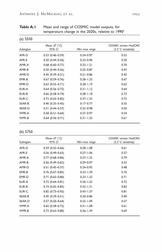
Anthony J. McMichael et al. 1623
Table A.1 Mean and range of COSMIC model outputs, fortemperature change in the 2020s, relative to 1990a
(a) S550
Mean dT (∞C) COSMIC version HadCM2Subregion 95% CI Min–max range (2.5 ∞C sensitivity)
AFR-D 0.53 (0.46–0.59) 0.24–0.97 0.53
AFR-E 0.50 (0.44–0.56) 0.23–0.96 0.50
AMR-A 0.68 (0.60–0.77) 0.32–1.21 0.70
AMR-B 0.50 (0.44–0.56) 0.25–0.87 0.47
AMR-D 0.45 (0.39–0.51) 0.21–0.86 0.42
EMR-B 0.67 (0.59–0.76) 0.28–1.25 0.67
EMR-D 0.63 (0.55–0.71) 0.28–1.19 0.62
EUR-A 0.64 (0.56–0.72) 0.31–1.12 0.64
EUR-B 0.66 (0.58–0.74) 0.28–1.18 0.73
EUR-C 0.73 (0.65–0.82) 0.37–1.23 0.72
SEAR-B 0.40 (0.35–0.45) 0.17–0.77 0.35
SEAR-D 0.51 (0.44–0.57) 0.22–0.98 0.50
WPR-A 0.58 (0.51–0.64) 0.27–0.97 0.54
WPR-B 0.64 (0.56–0.71) 0.31–1.25 0.61
(b) S750
Mean dT (∞C) COSMIC version HadCM2Subregion 95% CI Min–max range (2.5 ∞C sensitivity)
AFR-D 0.59 (0.52–0.66) 0.28–1.08 0.61
AFR-E 0.56 (0.49–0.63) 0.27–1.06 0.57
AMR-A 0.77 (0.68–0.86) 0.37–1.35 0.79
AMR-B 0.56 (0.49–0.62) 0.29–0.97 0.53
AMR-D 0.51 (0.45–0.57) 0.24–0.95 0.48
EMR-B 0.76 (0.67–0.85) 0.33–1.39 0.76
EMR-D 0.71 (0.63–0.80) 0.33–1.32 0.71
EUR-A 0.72 (0.64–0.81) 0.36–1.25 0.72
EUR-B 0.74 (0.65–0.83) 0.32–1.31 0.83
EUR-C 0.82 (0.73–0.92) 0.43–1.37 0.81
SEAR-B 0.45 (0.39–0.51) 0.20–0.86 0.40
SEAR-D 0.57 (0.50–0.64) 0.25–1.09 0.57
WPR-A 0.65 (0.58–0.72) 0.31–1.08 0.61
WPR-B 0.72 (0.63–0.80) 0.36–1.39 0.69

1624 Comparative Quantification of Health Risks
Table A.1 Mean and range of COSMIC model outputs, fortemperature change in the 2020s, relative to 1990a
(continued)
(c) Unmitigated emissions
Mean dT (∞C) COSMIC version HadCM2Subregion 95% CI Min–max range (2.5 ∞C sensitivity)
AFR-D 0.83 (0.73–0.92) 0.41–1.47 0.85
AFR-E 0.78 (0.70–0.87) 0.39–1.45 0.80
AMR-A 1.07 (0.96–1.19) 0.54–1.83 1.11
AMR-B 0.78 (0.69–0.86) 0.42–1.32 0.75
AMR-D 0.71 (0.63–0.79) 0.35–1.29 0.67
EMR-B 1.06 (0.94–1.17) 0.48–1.88 1.08
EMR-D 0.99 (0.88–1.11) 0.48–1.79 1.00
EUR-A 1.01 (0.90–1.12) 0.52–1.69 1.02
EUR-B 1.03 (0.92–1.15) 0.46–1.78 1.17
EUR-C 1.15 (1.03–1.27) 0.63–1.86 1.15
SEAR-B 0.63 (0.55–0.70) 0.29–1.17 0.56
SEAR-D 0.80 (0.70–0.89) 0.36–1.49 0.80
WPR-A 0.91 (0.81–1.00) 0.45–1.46 0.86
WPR-B 1.00 (0.89–1.11) 0.53–1.89 0.97
a Results of the simplified version of the HadCM2 model at medium (2.5 ∞C) sensitivity are shown forcomparison.

Anthony J. McMichael et al. 1625
Figure A.2 Mean and 95% CI of COSMIC model outputs for precipitationchange in the 2020s (relative to 1990), for each subregion undereach GHG emissions scenario
0.00
10.00
20.00
30.00
40.00
50.00
60.00
AFR-D AFR-E AMR-A AMR-B AMR-D EMR-B EMR-D EUR-A EUR-B EUR-C SEAR-B SEAR-D WPR- A WPR- B
Subregion
Pre
cip
itat
ion
ch
ang
e (m
m)
s550
s750
UE

1626 Comparative Quantification of Health Risks
Table A.2 Mean and range of COSMIC model outputs, for change inannual precipitation in the 2020s, relative to 1990a
(a) S550
Mean dPrecipn (mm) COSMIC version HadCM2Subregion 95% CI Min–max range (2.5 ∞C sensitivity)
AFR-D 8.18 (4.36–11.99) –15.8–43.88 4.92
AFR-E 6.71 (1.29–12.14) –31.83–57.55 14.88
AMR-A 12.01 (8.53–15.48) –10.38–54.00 13.56
AMR-B 9.17 (3.12–15.22) –41.47–60.79 5.28
AMR-D 20.03 (13.87–26.18) –31.17–71.40 33.48
EMR-B 3.45 (1.38–5.52) –7.10–25.61 2.52
EMR-D 9.05 (6.71–11.38) –1.83–32.97 5.76
EUR-A 9.94 (7.10–12.77) –9.58–43.69 14.88
EUR-B 3.33 (1.18–5.47) –9.55–15.18 7.56
EUR-C 11.50 (9.14–13.86) 0.72–37.68 12.48
SEAR-B 20.11 (11.05–29.16) –35.40–135.16 7.20
SEAR-D 25.87 (20.74–31.01) 4.40–71.19 17.64
WPR-A 14.39 (8.93–19.84) –33.56–68.61 1.32
WPR-B 14.82 (10.82–18.82) –7.36–55.37 13.44
(b) S750
Mean dPrecipn (mm) COSMIC version HadCM2Subregion 95% CI Min–max range (2.5 ∞C sensitivity)
AFR-D 9.25 (4.97–13.52) –17.66–48.79 5.60
AFR-E 7.67 (1.66–13.68) –31.02–63.98 16.83
AMR-A 13.52 (9.63–17.40) –11.79–60.07 15.43
AMR-B 10.32 (3.54–17.10) –46.11–67.59 5.97
AMR-D 22.61 (15.73–29.49) –34.64–79.40 37.88
EMR-B 4.24 (1.62–6.86) –7.89–37.10 3.03
EMR-D 10.33 (7.71–12.94) –2.05–36.66 6.47
EUR-A 11.19 (8.02–14.35) –10.85–48.58 16.87
EUR-B 3.74 (1.34–6.15) –10.82–16.88 8.60
EUR-C 12.95 (10.34–15.57) 0.83–41.90 14.18
SEAR-B 23.00 (12.69–33.32) –39.37–150.27 8.23
SEAR-D 29.15 (23.45–34.85) 5.07–79.18 19.94
WPR-A 16.22 (10.11–22.33) –37.30–76.29 1.49
WPR-B 16.70 (12.24–21.17) –8.19–62.12 15.22

Anthony J. McMichael et al. 1627
Table A.2 Mean and range of COSMIC model outputs, for change inannual precipitation in the 2020s, relative to 1990a
(continued)
(c) Unmitigated emissions
Mean dPrecipn (mm) COSMIC version HadCM2Subregion 95% CI Min–max range (2.5 ∞C sensitivity)
AFR-D 13.39 (7.44–19.35) –23.85–66.26 7.96
AFR-E 11.67 (3.69–19.64) –37.40–86.89 23.74
AMR-A 18.81 (13.49–24.13) –16.60–81.56 21.78
AMR-B 14.76 (5.64–23.88) –52.87–92.27 8.42
AMR-D 31.84 (22.38–41.31) –47.05–107.81 53.44
EMR-B 6.54 (2.75–10.34) –10.49–54.18 4.69
EMR-D 15.10 (11.37–18.82) –2.55–49.78 9.14
EUR-A 15.58 (11.24–19.92) –15.30–65.98 23.79
EUR-B 5.22 (1.90–8.53) –15.27–22.92 12.13
EUR-C 18.04 (14.50–21.58) 1.22–56.88 19.99
SEAR-B 32.75 (17.95–47.54) –53.44–220.93 11.62
SEAR-D 40.72 (33.00–48.44) 7.38–107.89 28.12
WPR-A 22.67 (14.23–31.11) –50.64–104.49 2.09
WPR-B 23.33 (17.18–29.47) –11.13–86.26 21.45
a Results of the simplified version of the HadCM2 model at medium (2.5 ∞C) sensitivity are shown forcomparison.

1628 Comparative Quantification of Health Risks
Appendix B: Literature review
For all impacts, we attempted to find all models that directly relatedclimate change to the selected health effects, either at the global or large-regional level. We describe all such models, and outline reasons for usingor not using them in the assessment. Note that the comments given relateto their relative suitability for generating the estimates required for thisassessment, rather than a general judgement on their merits. For theeffects of thermal extremes, we also include a summary of the study pop-ulations that were used to derive the heat and cold estimates used in thisassessment.
Where existing global or large scale regional models are not consid-ered appropriate (thermal extremes), or do not exist at all (diarrhoea andfloods), the literature search describes the procedure for identifying relevant studies from which to derive new quantitative climate–healthrelationships and generate models.

Anthony J. McMichael et al. 1629
Tabl
e B
.1R
esul
ts o
f lit
erat
ure
sear
ch fo
r ef
fect
s of
clim
ate
chan
ge o
n de
aths
due
to
ther
mal
ext
rem
esa Su
itabi
lity
for
gene
ratin
g Re
fere
nce
Met
hod
Inpu
tsRe
gion
Key
findi
ngs
estim
ates
for
thi
s as
sess
men
t
Lang
ford
and
R
egre
ssio
n m
odel
:Se
ason
al a
vera
ge d
TEn
glan
d an
d W
inte
r de
aths
avo
ided
:N
o po
pula
tion
grow
th,a
gein
g.Be
ntha
m (
1995
)m
onth
ly m
orta
lity
and
from
Uni
ted
Kin
gdom
W
ales
2010
:all
caus
e 33
01,I
HD
130
8,C
VD
429
No
seas
onal
adj
ustm
ent.
tem
pera
ture
ser
ies
scen
ario
s (W
arri
ck
2030
:all
caus
e 63
53,I
HD
255
0,C
VD
836
Loca
l rat
her
than
glo
bal
(flu
incl
uded
)an
d Ba
rrow
199
1)20
50:a
ll ca
use
8922
,IH
D 3
631,
CV
D 1
187
Mar
tens
(19
98a)
MIA
SMA
v1.0
—em
piri
cal-
ECH
AM
1-A
,UK
TR
,C
ause
+ag
e
Cha
nges
in m
orta
lity
rate
s fo
r C
VD
(<6
5),
Lack
of
cont
rol f
or s
easo
nal
stat
istic
al m
odel
,G
FDL8
9 (IP
CC
sp
ecifi
c.C
VD
(>6
5),r
espi
rato
ry,a
nd t
otal
mor
talit
yva
riat
ions
,per
haps
m
eta-
anal
ysis
.A s
ingl
e
scen
ario
s)G
loba
l—N
et r
educ
tions
in m
orta
lity
in a
ll ci
ties
over
-est
imat
ing
heat
effe
cts
tem
pera
ture
-mor
talit
y20
citi
esex
cept
res
pira
tory
mor
talit
y in
a fe
w c
ities
re
latio
nshi
p w
as a
pplie
dto
all
citie
s
McM
icha
el e
t al
.M
IASM
Av.
1.0—
as fo
r H
adC
M2,
ense
mbl
e G
loba
l—N
et r
educ
tions
in m
orta
lity
in a
ll ci
ties
As
for
Mar
tens
(19
98a)
(200
0b)
Mar
tens
(19
98a)
mea
n+
Had
CM
320
citi
esex
cept
Ath
ens,
due
to d
ecre
ases
in
win
ter
mor
talit
y
TH
ER
MA
LE
XT
RE
ME
S
Info
rmat
ion
sour
ces:
•al
l re
leva
nt p
aper
s ci
ted
in I
PCC
(20
01a)
•M
edlin
e se
arch
for
all
refe
renc
es (
1966
–200
2) c
onta
inin
g th
e te
rms
“tem
pera
ture
”; “
mor
talit
y”;
“car
diov
ascu
lar
dise
ase”
(or
CV
D);
“re
spir
ator
y”;
“wea
ther
”
•re
fere
nces
cit
ed i
n th
ese
pape
rs.
cont
inue
d

1630 Comparative Quantification of Health RisksTa
ble
B.1
Res
ults
of
liter
atur
e se
arch
for
effe
cts
of c
limat
e ch
ange
on
deat
hs d
ue t
o th
erm
al e
xtre
mes
a(c
ontin
ued)
Suita
bilit
y fo
r ge
nera
ting
Refe
renc
eM
etho
dIn
puts
Regi
onKe
y fin
ding
ses
timat
es f
or t
his
asse
ssm
ent
Kal
kste
in a
nd
Mod
el d
eriv
ed f
rom
G
CM
sce
nari
os,n
o G
loba
l—Si
gnifi
cant
incr
ease
s in
hea
t-re
late
d M
etho
ds u
sed
rely
on
syno
ptic
Smoy
er (
1993
)ob
serv
ed r
elat
ions
hip
dow
nsca
ling
27 c
ities
mor
talit
y un
der
vari
ous
clim
ate
chan
ge
clas
sific
atio
n of
loca
l air
be
twee
n sy
nopt
ic a
ir
scen
ario
s,w
ith o
r w
ithou
t m
asse
s;th
eref
ore
cann
ot b
e m
asse
s an
d m
orta
lity
accl
imat
izat
ion,
proj
ecte
d fo
r al
l citi
esdi
rect
ly r
elat
ed t
o ch
ange
s in
tem
pera
ture
des
crib
ed
by c
limat
e sc
enar
ios
Kal
kste
in a
nd
Mod
el d
eriv
ed f
rom
G
CM
sce
nari
os,n
o 44
citi
es in
In
crea
ses
in h
eat-
rela
ted
mor
talit
y ar
e M
etho
ds u
sed
rely
on
syno
ptic
G
reen
e (1
997)
obse
rved
rel
atio
nshi
p do
wns
calin
gth
e U
SAm
uch
larg
er o
vera
ll th
an d
ecre
ases
in
clas
sific
atio
n of
loca
l air
betw
een
syno
ptic
air
co
ld-r
elat
ed m
orta
lity
mas
ses;
ther
efor
e ca
nnot
be
m
asse
s an
d m
orta
lity
dire
ctly
rel
ated
to
chan
ges
in t
empe
ratu
re d
escr
ibed
by
clim
ate
scen
ario
s
Dun
can
et a
l.M
odel
der
ived
fro
m
Clim
ate
scen
ario
s fo
r 10
citi
es
240–
1140
add
ition
al h
eat-
rela
ted
Cou
ntry
spe
cific
(199
7)ob
serv
ed r
elat
ions
hip
C
anad
ain
Can
ada
deat
hs/y
ear
in M
ontr
eal b
y 20
50;2
30–1
220
betw
een
syno
ptic
air
ad
ditio
nal d
eath
s in
Tor
onto
,ass
umin
g m
asse
s an
d m
orta
lity
no a
cclim
atiz
atio
n.N
o cl
imat
e/m
orta
lity
rela
tions
hip
in s
ome
citie
s
Gue
st e
t al
.R
egre
ssio
n m
odel
:C
SIRO
Mar
k 2
mod
el,
5 ci
ties
in
Net
dec
reas
e in
hea
t-re
late
d m
orta
lity,
Cou
ntry
spe
cific
(199
9)da
ily m
orta
lity
and
CO
2do
ublin
g;hi
gh
Aus
tral
iapa
rtic
ular
ly in
the
age
gro
up ≥
65
syno
ptic
indi
ces
and
low
sce
nari
os
year
s;ra
nge
of 4
7–62
few
er d
eath
s/ye
ar in
es
timat
ed
all 5
citi
es.S
igni
fican
t in
crea
se in
sum
mer
de
aths
in S
ydne
y (7
6–23
9)
Des
sai (
2003
)Em
piri
cal s
tatis
tical
2
regi
onal
clim
ate
Lisb
on,
Hea
t-re
late
d de
ath
rate
s in
crea
se b
y C
ount
ry s
peci
ficm
odel
,obs
erve
d-m
odel
s—PR
OM
ES
Port
ugal
57–1
13%
by
2020
s,by
97–
255%
by
2050
s.ex
pect
edan
d H
adR
M2
Acc
limat
izat
ion
assu
mpt
ions
,red
uce
estim
ates
Key
:C
VD
,car
diov
ascu
lar
dise
ase;
IHD
,isc
haem
ic h
eart
h di
seas
e;G
CM
,glo
bal c
limat
e m
odel
.a
A t
otal
of
76 o
ther
pub
licat
ions
wer
e no
t us
ed,e
ither
bec
ause
the
y w
ere
anal
yses
of
spec
ific
epis
odes
(35
stu
dies
),or
bec
ause
the
y di
d no
t m
atch
the
cri
teri
a ou
tline
d ab
ove
(41
stud
ies)
.

Anthony J. McMichael et al. 1631
ESTIMATES OF TEMPERATURE–MORTALITY RELATIONSHIP
Table B.2 below lists all studies (n=4) that meet the following criteriafor inclusion in the meta-analysis. The study:
• uses daily time-series methods to analyse the relationship betweendaily mean temperature and mortality;
• Reports a coefficient from log linear regression that estimates the per-centage changes in mortality per degree centigrade change in temper-ature, above a reported threshold temperature;
• has controls for the following confounders: season, air pollution andinfluenza;
• is published in English language only; and
• reports confidence intervals around the coefficient and is within therange of other reported estimates.
The studies are classified according to climate zone. The Netherlandspopulation is used to approximate a population in the “cold” zone asthere are no other appropriate time-series studies.
Note that some studies are included that are not yet published.However,
• they are the only studies available that provide estimates for devel-oping country populations; and
• the results will be submitted to peer reviewed journals and themethods are at least as rigorous as those applied in previous publishedstudies.
All estimates have been rounded to one decimal place. Where morethan one estimate was available, the average estimate was calculated.

1632 Comparative Quantification of Health Risks
Tabl
e B
.2R
esul
ts o
f lit
erat
ure
sear
ch fo
r te
mpe
ratu
re–m
orta
lity
rela
tions
hip
Popu
latio
n/%
cha
ngea
per
Cut-p
oint
% c
hang
eape
rCu
t-poi
nt
clim
ate
zone
Age
Caus
e of
dea
th1
∞C d
ecre
ase
(ºC)
Lag
1ºC
incr
ease
(º
C)La
gRe
fere
nce
CO
LDH
EAT
Net
herl
ands
All
All
caus
e0.
4116
.57–
151.
2316
.51–
2K
unst
et
al.(
1993
)
Net
herl
ands
All
CV
D0.
4616
.57–
151.
1316
.51–
2K
unst
et
al.(
1993
)
Net
herl
ands
All
Res
pira
tory
1.43
16.5
7–15
3.11
16.5
1–2
Kun
st e
t al
.(19
93)
CO
LD
CV
D0.
51.
1
Bulg
aria
Sofia
All
All
2.69
(0.
88–4
.54)
–20–
131.
93 (
1.41
–2.4
5)17
0–2
ISO
TH
UR
M (
fort
hcom
ing)
Chi
le Sant
iago
All
All
5.21
(3.
55–6
.89)
110–
130.
92 (
0.44
–1.3
1)16
0–
2IS
OT
HU
RM
(fo
rthc
omin
g)
Slov
enia
Ljub
ljana
All
All
0.77
(–0
.16–
1.70
)7
0–13
2.25
(1.
09–3
.42)
17
0–2
ISO
TH
UR
M (
fort
hcom
ing)
Sout
h A
fric
aC
ape
Tow
nA
ll A
ll3.
32 (
2.89
–3.7
5)19
0–13
1.02
(–0
.32–
2.38
)21
0–2
ISO
TH
UR
M (
fort
hcom
ing)
Spai
nM
adri
dA
ll A
ll 1.
720
7 0.
9720
0–1
Alb
erdi
(19
98)
Vale
ncia
All
All
3.2
(1.8
–4.6
)15
7–14
3.6
(1.2
–6.0
)24
1–
2Ba
llest
er e
t al
.(19
97)
Vale
ncia
>70
All
3.7
(2.1
–5.4
)15
7–14
5.0
(2.1
–8.0
)24
1–
2Ba
llest
er e
t al
.(19
97)
Vale
ncia
All
CV
D4.
3 (2
.1–6
.4)
157–
142.
3 (–
1.5–
4.5)
24
1–2
Balle
ster
et
al.(
1997
)Va
lenc
iaA
llC
VD
1.5
(–0.
3–3.
3)15
3–6
2.9
(–0.
4–7.
4)24
3–
6Ba
llest
er e
t al
.(19
97)
Vale
ncia
All
Res
pira
tory
1.7
(–0.
4–6.
0)15
7–14
5.7
(–2.
9–8.
2)24
1–
2Ba
llest
er e
t al
.(19
97)

Anthony J. McMichael et al. 1633
TEM
PER
ATE
CV
D2.
92.
6
Braz
ilSã
o Pa
ulo
All
All
caus
e3.
92 (
3.43
–4.4
0)19
0–13
2.28
(2.
11–3
.66)
23
0–2
ISO
TH
UR
M (
fort
hcom
ing)
São
Paul
o≥6
5A
ll ca
use
5.5
200–
212.
5 (2
.1–2
.8)
200–
1G
ouve
ia e
t al
.(20
03)
El S
alva
dor
San
Salv
ador
All
All
caus
e–1
3.5
(–32
.35–
10.9
)23
0–13
1.59
(0.
86–2
.32)
23
0–2
ISO
TH
UR
M (
fort
hcom
ing)
Mex
ico
Mex
ico
City
All
All
caus
e8.
60 (
7.86
–9.3
4)15
0–13
0.6
(0.2
1–1.
00)
180–
2IS
OT
HU
RM
(fo
rthc
omin
g)
Mex
ico
Mon
terr
eyA
ll A
ll ca
use
5.54
(4.
52–6
.58)
170–
1319
.85
(14.
69–2
5.25
)31
0–2
ISO
TH
UR
M (
fort
hcom
ing)
Tha
iland
Bang
kok
All
All
caus
e4.
13 (
1.71
–6.6
1)28
0–13
7.66
(5.
87–9
.47)
30
0–2
ISO
TH
UR
M (
fort
hcom
ing)
WA
RM
HU
MID
All
All
caus
e5.
55.
7
Indi
a Del
hiA
ll A
ll ca
use
1.36
(0.
56–2
.16)
190–
133.
03 (
2.48
–3.5
8)28
0–
2IS
OT
HU
RM
(fo
rthc
omin
g)
HO
T D
RY
All
All
caus
e1.
43.
0
CV
DC
ardi
ovas
cula
r di
seas
e.a
% c
hang
e=
(RR
-1)
¥10
0.

1634 Comparative Quantification of Health Risks
Tabl
e B
.3R
esul
ts o
f lit
erat
ure
sear
ch fo
r ef
fect
s of
clim
ate
chan
ge o
n di
arrh
oeaa
Glo
bal m
odel
s re
latin
g Lo
cal s
tudi
es q
uant
itativ
ely
Loca
l stu
dies
sho
win
g se
ason
al
clim
ate/
clim
ate
rela
ting
all-c
ause
dia
rrho
ea
patte
rns
in a
ll- o
r m
ultip
le-c
ause
Lo
cal s
tudi
es s
how
ing
path
ogen
-spe
cific
chan
ge t
o di
arrh
oea
to t
empe
ratu
redi
arrh
oea
(non
-qua
ntita
tive)
asso
ciatio
ns w
ith c
limat
e
Non
eC
heck
ley
et a
l.(2
000)
;A
njan
eyul
u et
al.
(197
5);B
ecke
r Sh
owin
g as
soci
atio
n:Si
ngh
et a
l.(2
001)
(198
1);B
rew
ster
and
Gre
enw
ood
Ade
gbol
a et
al.
(199
4);A
dkin
s et
al.
(198
7);A
ggar
wal
et
al.(
1983
);A
nsar
i(1
993)
;Dea
n an
d Jo
nes
(197
2);
et a
l.(1
991)
;Arm
ah e
t al
.(19
94);
Bear
ds a
nd G
raha
m (
1995
);Bo
ckem
uhl
Hog
e et
al.
(199
6);J
in e
t al
.(1
976)
;Cal
leja
s et
al.
(199
9);C
hakr
avar
ti et
al.
(199
2);C
han
et a
l.(1
998)
;(1
996)
;Lin
g an
d C
heng
(19
93);
Cha
udhu
ry e
t al
.(19
96);
Coo
k et
al.
(199
0);C
unlif
fe e
t al
.(19
98);
da R
osa
eM
erlin
et
al.(
1986
);Pa
rash
ar
Silv
a et
al.
(200
1);D
ougl
as a
nd K
urie
n (1
997)
;Ebe
rhar
d et
al.
(199
9);F
ujita
et
al.
(199
9);P
info
ld e
t al
.(19
91);
(199
0);H
enry
and
Bar
thol
omew
(19
90);
Hir
schl
et
al.(
1987
);Ija
z et
al.
Rob
ins-
Brow
ne (
1984
);R
oush
am(1
985)
;Kon
no e
t al
.(19
83);
Laur
sen
et a
l.(1
994)
;LeB
aron
et
al.(
1990
);an
d M
asci
etay
lor
(199
5);S
aidi
M
alak
ooti
et a
l.(1
997)
;Muh
uri (
1996
);M
usa
et a
l.(1
999)
;Nch
ito e
t al
.et
al.
(199
7);S
awch
uk (
1993
);(1
998)
;Par
asha
r et
al.
(199
8a,1
998b
);Pa
zzag
lia e
t al
.(19
93);
Puro
hit
et a
l.Sh
aikh
et
al.(
1990
);Su
tra
et a
l.(1
998)
;Qia
o et
al.
(199
9);R
am e
t al
.(19
90a,
1990
b);R
eyes
et
al.(
1996
);(1
990)
;Tsu
kam
oto
et a
l.(1
978)
;R
ytle
wsk
a et
al.
(200
0);S
allo
n et
al.
(199
1);S
ethi
et
al.(
1984
);Sh
ahid
et
al.
Van
den
Broe
ck e
t al
.(19
93);
(198
7);S
hkar
in e
t al
.(19
83);
Sorv
illo
et a
l.(1
998)
;Ste
wie
n et
al.
(199
1);
Will
iam
s et
al.
(198
6);Y
ang
Stin
tzin
g et
al.
(198
1);T
swan
a et
al.
(199
0);U
tsal
o et
al.
(199
1);V
laso
v et
al.
et a
l.(1
990)
(198
3);W
ilcox
et
al.(
1992
);W
uhib
et
al.(
1994
)
Faili
ng t
o fin
d as
soci
atio
n:Bi
shop
et
al.(
2001
);C
onte
as e
t al
.(19
98);
Varo
li et
al.
(198
9)
aA
tot
al o
f 59
7 pu
blic
atio
ns w
ere
reje
cted
on
the
basi
s of
lack
of
info
rmat
ion
in a
bstr
act,
or ir
rele
vanc
e to
qua
ntita
tive
asse
ssm
ent
(mai
nly
revi
ews,
clin
ical
and
labo
rato
ry s
tudi
es).
DIA
RR
HO
EA
Info
rmat
ion
sour
ces:
•al
l re
leva
nt p
aper
s ci
ted
in I
PCC
(20
01a)
•M
edlin
e se
arch
for
all
refe
renc
es (
1966
–200
2) c
onta
inin
g th
e te
rms
“Dia
rrho
ea (
or d
iarr
hea)
and
clim
ate
(or
clim
atic
)ch
ange
”; “
diar
rhoe
a (o
r di
arrh
ea)
and
clim
ate”
; “d
iarr
hoea
(or
dia
rrhe
a) a
nd w
eath
er”
•re
fere
nces
cit
ed i
n th
ese
pape
rs.
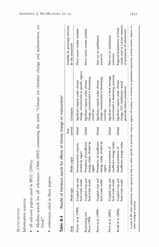
Anthony J. McMichael et al. 1635
Tabl
e B
.4R
esul
ts o
f lit
erat
ure
sear
ch fo
r ef
fect
s of
clim
ate
chan
ge o
n m
alnu
triti
ona
Area
Su
itabi
lity
for
gene
ratin
g es
timat
es
Stud
yM
odel
typ
eM
odel
out
put
cove
red
Conc
lusio
nsfo
r th
is as
sess
men
t
Fisc
her
et a
l.(1
994)
Cou
pled
cro
p an
dSo
cioe
cono
mic
impa
cts,
Glo
bal
Sign
ifica
nt im
pact
s un
der
clim
ate
Mor
e re
cent
mod
els
avai
labl
efo
od t
rade
mod
eldi
vide
d by
reg
ion
chan
ge,c
once
ntra
ted
in s
peci
fic r
egio
ns
Ros
enzw
eig
and
Cou
pled
cro
p an
d Pr
eval
ence
of
insu
ffici
ent
Glo
bal
Sign
ifica
nt im
pact
s un
der
clim
ate
Mor
e re
cent
mod
els
avai
labl
ePa
rry
(199
4)fo
od t
rade
mod
elen
ergy
inta
ke,d
ivid
ed b
y ch
ange
,con
cent
rate
d in
dev
elop
ing
regi
onco
untr
ies
Parr
y et
al.
(199
9)C
oupl
ed c
rop
and
Prev
alen
ce o
f in
suffi
cien
t G
loba
lSi
gnifi
cant
impa
cts
unde
r cl
imat
e N
ot r
un o
n st
abili
zatio
n fo
od t
rade
mod
elen
ergy
inta
ke,d
ivid
ed b
ych
ange
,con
cent
rate
d in
dev
elop
ing
scen
ario
sre
gion
coun
trie
s
Parr
y et
al.
(200
1)C
oupl
ed c
rop
and
Glo
bal p
reva
lenc
e of
G
loba
lSi
gnifi
cant
incr
ease
in fo
od s
hort
age,
Not
run
on
stab
iliza
tion
food
tra
de m
odel
insu
ffici
ent
ener
gy in
take
conc
entr
ated
in d
evel
opin
g co
untr
ies
scen
ario
s
Arn
ell e
t al
.(20
02)
Cou
pled
cro
p an
d G
loba
l pre
vale
nce
of
Glo
bal
Sign
ifica
nt im
pact
s un
der
clim
ate
Reg
iona
l bre
akdo
wns
of
thes
e fo
od t
rade
mod
elin
suffi
cien
t en
ergy
inta
kech
ange
,CO
2st
abili
zatio
n w
ould
re
sults
use
d as
a p
roxy
mea
sure
ge
nera
lly r
educ
e pr
eval
ence
of p
reva
lenc
e of
mal
nutr
ition
aA
tot
al o
f 28
1 ot
her
publ
icat
ions
wer
e re
ject
ed a
s th
ey a
re e
ither
spe
cific
to
part
icul
ar c
rops
or
regi
ons
(10
stud
ies)
,or
irre
leva
nt t
o qu
antit
ativ
e as
sess
men
t (m
ainl
y re
view
s,im
pact
s on
othe
r ec
olog
ical
sys
tem
s).
MA
LN
UT
RIT
ION
Info
rmat
ion
sour
ces:
•al
l re
leva
nt p
aper
s ci
ted
in I
PCC
(20
01a)
•M
edlin
e se
arch
for
all
refe
renc
es (
1966
–200
2) c
onta
inin
g th
e te
rms
“Clim
ate
(or
clim
atic
) ch
ange
and
mal
nutr
itio
n (o
rfo
od)”
•re
fere
nces
cit
ed i
n th
ese
pape
rs.

1636 Comparative Quantification of Health Risks
Tabl
e B
.5R
esul
ts o
f lit
erat
ure
sear
ch fo
r ef
fect
s of
clim
ate
chan
ge o
n de
aths
and
inju
ries
due
to
flood
s an
d la
ndsl
ides
a
Larg
e ar
ea s
tudi
es
Glo
bal o
r la
rge
regi
onal
mod
els
Glo
bal m
odel
s pr
edict
ing
Caus
es o
f flo
od e
vent
s w
hich
Ca
uses
of
land
slide
s w
hich
cau
sed
quan
titat
ively
rela
ting
pred
ictin
g cl
imat
e ch
ange
effe
cts
oncl
imat
e ch
ange
ca
used
dea
ths
and/
or in
jurie
s de
aths
and
/or
inju
ries
repo
rted
inpr
ecip
itatio
n or
sea
-leve
lfre
quen
cy o
f ex
trem
e pr
ecip
itatio
n ef
fect
s on
fre
quen
cy
repo
rted
in t
he E
M-D
AT
the
EM-D
AT e
nhan
ced
rise
to d
eath
s/in
jurie
sev
ents
or
inla
nd fl
oodi
ngof
coa
stal
floo
ding
enha
nced
dat
abas
e (1
980–
1999
)da
taba
se (
1980
–199
9)
Non
eBo
oij (
2002
),w
este
rn E
urop
eBa
arse
(19
95)
Ass
ocia
ted
with
pre
cipi
tatio
n63
ass
ocia
ted
with
pre
cipi
tatio
n
Fow
ler
and
Hen
ness
y (1
995)
,H
ooze
man
s an
d 2
with
hig
h tid
es a
nd s
torm
10
ass
ocia
ted
with
oth
er c
ause
s (e
.g.
spec
ific
loca
tions
wor
ldw
ide
Hul
sbur
gen
(199
5)su
rges
land
slid
es a
t m
ines
,clif
fs c
olla
psin
g)
Jone
s an
d R
eid
(200
1) U
nite
d N
icho
lls a
nd M
imur
a 19
oth
er c
ause
s (e
.g.c
yclo
nes,
115
with
out
spec
ific
info
rmat
ion
Kin
gdom
(199
8)ic
e m
elt,
dam
s bu
rstin
g)on
cau
se
Mill
y et
al.
(200
2) s
peci
fic
Nic
holls
et
al.(
1999
)55
9 w
ithou
t sp
ecifi
c in
form
atio
n lo
catio
ns w
orld
wid
eon
cau
se
Palm
er a
nd R
alsa
nen
(200
2)
nort
hern
Eur
ope,
Sout
h-Ea
st A
sia
aA
tot
al o
f 34
2 ot
her
publ
icat
ions
wer
e re
ject
ed a
s th
ey a
re e
ither
spe
cific
to
part
icul
ar r
egio
ns,o
r ir
rele
vant
to
quan
titat
ive
asse
ssm
ent
(mai
nly
revi
ews,
desc
ript
ions
of
spec
ific
even
ts).
CO
AST
AL
AN
DIN
LA
ND
FLO
OD
ING
Info
rmat
ion
sour
ces:
•al
l re
leva
nt p
aper
s ci
ted
in I
PCC
(20
01a)
•IS
I-W
eb o
f Sc
ienc
e se
arch
for
“Fl
oods
(or
floo
ding
) an
d cl
imat
e (o
r cl
imat
ic)
chan
ge”;
“Fl
oods
(or
floo
ding
) an
d he
alth
(or
deat
h or
inj
ury
or m
orta
lity)
”; “
Ext
rem
e pr
ecip
itat
ion
and
heal
th (
or d
eath
or
inju
ry o
r m
orta
lity)
”
•M
edlin
e se
arch
for
“Fl
oods
(or
floo
ding
) an
d cl
imat
e (o
r cl
imat
ic)
chan
ge”
•R
efer
ence
s ci
ted
in t
hese
pap
ers
•In
spec
tion
of
desc
ript
ions
of
all
flood
eve
nts
liste
d in
EM
-DA
T e
nhan
ced
data
base
198
0–19
99 (
EM
-DA
T 2
002)
.
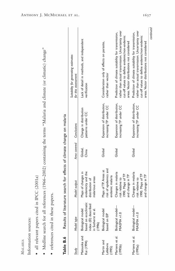
Anthony J. McMichael et al. 1637
Tabl
e B
.6R
esul
ts o
f lit
erat
ure
sear
ch fo
r ef
fect
s of
clim
ate
chan
ge o
n m
alar
ia
Suita
bilit
y fo
r ge
nera
ting
estim
ates
St
udy
Mod
el t
ype
Mod
el o
utpu
tAr
ea c
over
edCo
nclu
sions
for
this
asse
ssm
ent
Mat
suok
a an
dBi
olog
ical
mod
el
Map
s of
cha
nges
in
Glo
bal,
Cha
nge
in d
istr
ibut
ion
Lack
of
deta
il in
met
hods
,and
inde
pend
ent
Kai
(19
94)
base
d on
eco
clim
atic
en
dem
icity
and
the
C
hina
patt
erns
und
er C
Cve
rific
atio
nin
dex
(EI)
desc
ribe
d di
stri
butio
n of
in
Sut
hers
t et
al.
mal
ario
us a
reas
(199
6)
Mar
tin a
nd
Biol
ogic
al m
odel
M
aps
of T
P.A
reas
at
Glo
bal
Expa
nsio
n of
dis
trib
utio
n,C
onsi
dera
tion
only
of
effe
cts
on p
aras
ite,
Lefe
bvre
ba
sed
on E
IPri
sk o
f ep
idem
ics
and
incr
easi
ng T
P un
der
CC
rath
er t
han
vect
or(1
995)
ende
mic
mal
aria
Mar
tens
et
al.
Biol
ogic
al m
odel
—C
hang
es in
mal
aria
G
loba
lEx
pans
ion
of d
istr
ibut
ion,
Pred
ictio
n of
clim
ate
suita
bilit
y fo
r tr
ansm
issi
on,
(199
5b)
MIA
SMA
v1.0
risk
rel
ativ
e to
in
crea
sing
TP
unde
r C
Cra
ther
tha
n ac
tual
tra
nsm
issi
on.U
ncer
tain
ty o
ver
1990
.Map
s of
TP
cut-
off
valu
es t
o de
fine
ende
mic
/non
-end
emic
an
d ch
ange
in T
Par
eas.
Vect
or d
istr
ibut
ions
not
con
side
red
Mar
tens
et
al.
Biol
ogic
al m
odel
—C
hang
es in
mal
aria
G
loba
lEx
pans
ion
of d
istr
ibut
ion,
Pred
ictio
n of
clim
ate
suita
bilit
y fo
r tr
ansm
issi
on,
(199
5a)
MIA
SMA
v1.0
risk
rel
ativ
e to
in
crea
sing
TP
unde
r C
Cra
ther
tha
n ac
tual
tra
nsm
issi
on.U
ncer
tain
ty o
ver
1990
.Map
s of
TP
cu
t-of
f va
lues
to
defin
e en
dem
ic/n
on-e
ndem
ic
and
chan
ge in
TP
area
s.Ve
ctor
dis
trib
utio
ns n
ot c
onsi
dere
d
MA
LA
RIA
Info
rmat
ion
sour
ces:
•al
l re
leva
nt p
aper
s ci
ted
in I
PCC
(20
01a)
•M
edlin
e se
arch
for
all
refe
renc
es (
1966
–200
2) c
onta
inin
g th
e te
rms
“Mal
aria
and
clim
ate
(or
clim
atic
) ch
ange
”
•re
fere
nces
cit
ed i
n th
ese
pape
rs.
cont
inue
d

1638 Comparative Quantification of Health Risks
Tabl
e B
.6R
esul
ts o
f lit
erat
ure
sear
ch fo
r ef
fect
s of
clim
ate
chan
ge o
n m
alar
ia (
cont
inue
d) Suita
bilit
y fo
r ge
nera
ting
estim
ates
St
udy
Mod
el t
ype
Mod
el o
utpu
tAr
ea c
over
edCo
nclu
sions
for
this
asse
ssm
ent
Brya
n et
al.
CLI
MEX
mod
el
Vect
or d
istr
ibut
ions
N
orth
ern
Cha
nge
in d
istr
ibut
ion
Sing
le v
ecto
r,lo
cal r
athe
r th
an g
loba
l pre
dict
ions
(1
996)
only
Aus
tral
iaun
der
CC
Jett
en e
t al
.Bi
olog
ical
mod
el—
Map
s of
TP
and
Glo
bal
Expa
nsio
n of
dis
trib
utio
n,Pr
edic
tion
of c
limat
e su
itabi
lity
for
tran
smis
sion
,(1
996)
MIA
SMA
v1.
0ch
ange
in T
Pin
crea
sing
TP
unde
r C
Cra
ther
tha
n ac
tual
tra
nsm
issi
on.U
ncer
tain
ty o
ver
cut-
off
valu
es t
o de
fine
ende
mic
/non
-end
emic
ar
eas.
Vect
or d
istr
ibut
ions
not
con
side
red
Mar
tens
M
IASM
A v
1.0
Map
s of
TP
and
chan
ge
Glo
bal
Expa
nsio
n of
dis
trib
utio
n,Pr
edic
tion
of c
limat
e su
itabi
lity
for
tran
smis
sion
,(1
997)
in T
P,P.
vivax
and
incr
easi
ng T
P un
der
CC
rath
er t
han
actu
al t
rans
mis
sion
.Unc
erta
inty
ove
r P.
falci
paru
mcu
t-of
f va
lues
to
defin
e en
dem
ic/n
on-e
ndem
ic
area
s.Ve
ctor
dis
trib
utio
ns n
ot c
onsi
dere
d
Lind
say
and
MIA
SMA
v1.
0—M
aps—
epid
emic
A
fric
an
Incr
ease
in la
titud
e R
egio
nal p
roje
ctio
ns o
nly
Mar
tens
bi
olog
ical
pote
ntia
lH
ighl
ands
unde
r C
C(1
998)
mod
el b
ased
on
vect
oria
l cap
acity
Rog
ers
Empi
rica
l sta
tistic
al
Map
s of
dis
trib
utio
n So
uthe
rn
Cha
nge
in d
istr
ibut
ion
Reg
iona
l pro
ject
ions
onl
y(1
996)
map
ping
of A
noph
eles
gam
biae
Afr
ica
unde
r C
C
Mar
tens
et
al.
Biol
ogic
al m
odel
,M
aps
of T
P,m
aps
of
Glo
bal
Expa
nsio
n of
dis
trib
utio
n,Pr
edic
tion
of c
limat
e su
itabi
lity
for
tran
smis
sion
,(1
999)
over
layi
ng a
chan
ges
in s
easo
nal
incr
easi
ng T
P un
der
CC
rath
er t
han
actu
al t
rans
mis
sion
popu
latio
n gr
id.
tran
smis
sion
,add
ition
alM
IASM
A v
2.0
popu
latio
n at
ris
k

Anthony J. McMichael et al. 1639
Arn
ell e
t al
.Bi
olog
ical
mod
el,
Map
s of
cha
nges
in P
.G
loba
lEx
pans
ion
of d
istr
ibut
ion,
Pred
ictio
n of
clim
ate
suita
bilit
y fo
r tr
ansm
issi
on,
(200
2)ov
erla
ying
a
falci
paru
mT
P,po
pula
tion
incr
easi
ng T
P un
der
CC
ra
ther
tha
n ac
tual
tra
nsm
issi
onpo
pula
tion
grid
.at
ris
k,se
ason
s su
itabl
e M
IASM
A v
2.0
for
tran
smis
sion
rel
ativ
e to
196
1–19
90
Rog
ers
and
Empi
rica
l-sta
tistic
al
Cha
nges
in p
opul
atio
ns
Glo
bal
App
roxi
mat
ely
no
Add
ition
al p
opul
atio
n at
ris
k ±
25 m
illio
n.Va
lidat
ion
Ran
dolp
h m
odel
at r
isk:
P.fa
lcipa
rum
chan
ge in
dis
trib
utio
n of
mod
el d
eriv
ed f
rom
a s
ubse
t of
the
dat
a ag
ains
t(2
000)
unde
r cl
imat
e ch
ange
the
rem
aini
ng o
bser
vatio
ns.(
Use
d to
info
rm
unce
rtai
nty
rang
e ar
ound
the
pro
ject
ions
)
Tans
er e
t al
.M
AR
A b
iolo
gica
l/ C
hang
es in
pop
ulat
ions
A
fric
aEx
pans
ion
in p
opul
atio
nBi
olog
ical
mod
el b
ased
on
loca
lized
fiel
d st
udie
s,(2
003)
stat
istic
al m
odel
at
ris
k—m
onth
s su
itabl
eat
ris
k un
der
CC
used
to
pred
ict
popu
latio
n at
ris
k an
d nu
mbe
rs o
f (C
raig
et
al.1
999)
for
tran
smis
sion
mon
ths
at r
isk
thro
ugho
ut A
fric
a,bu
t no
t el
sew
here
.Pot
entia
l for
dev
elop
ing
into
pre
dict
ions
of in
cide
nce.
Valid
ated
aga
inst
det
aile
d in
depe
nden
tda
ta s
et.(
Use
d to
det
erm
ine
mid
-ran
ge e
stim
ates
of p
opul
atio
n at
ris
k,as
a r
elat
ive
mea
sure
of
chan
ge in
inci
denc
e)
Key
:C
C,c
limat
e ch
ange
;EIP
,ext
rins
ic in
cuba
tion
peri
od;T
P,tr
ansm
issi
on p
oten
tial (
also
cal
led
EP,e
pide
mic
pot
entia
l).a
A f
urth
er 4
1 pu
blic
atio
ns w
ere
reje
cted
due
to
lack
of
rele
vanc
e fo
r m
akin
g gl
obal
pro
ject
ions
(m
ainl
y re
view
s,lo
cal s
tudi
es).

1640 Comparative Quantification of Health Risks
Tabl
e B
.7R
esul
ts o
f lit
erat
ure
sear
ch fo
r pr
ojec
ted
effe
cts
of c
limat
e ch
ange
on
deng
uea
Suita
bilit
y fo
r ge
nera
ting
Stud
yM
odel
typ
eM
odel
out
put
Area
cov
ered
Conc
lusio
nses
timat
es f
or t
his
asse
ssm
ent
Mar
tens
et
al.
Biol
ogic
al m
odel
sum
mar
izin
g M
aps
of c
hang
e in
G
loba
lLa
rge
incr
ease
in
Rel
atio
nshi
p be
twee
n T
P an
d (1
997)
clim
ate
effe
cts
on v
ecto
r an
d ep
idem
ic p
oten
tial
tran
smis
sion
pot
entia
l with
di
seas
e in
cide
nce
not
char
acte
rize
d.pa
rasi
te p
opul
atio
n dy
nam
ics
unde
r cl
imat
e sm
all t
empe
ratu
re in
crea
seU
ncer
tain
ty o
ver
defin
ition
s fo
r M
IASM
A v
1.0,
coup
led
with
ch
ange
thre
shol
d T
P to
defi
ne li
mits
of
DEN
SIM
mod
el o
f Fo
cks
dist
ribu
tion
et a
l.(1
995)
DE
NG
UE
Info
rmat
ion
sour
ces:
•al
l re
leva
nt p
aper
s ci
ted
in I
PCC
(20
01a)
•M
edlin
e se
arch
for
all
refe
renc
es (
1966
–200
2) c
onta
inin
g th
e te
rms
“Den
gue
and
clim
ate
(or
clim
atic
) ch
ange
”
•Se
cond
ary
refe
renc
es c
ited
in
thes
e pa
pers
.
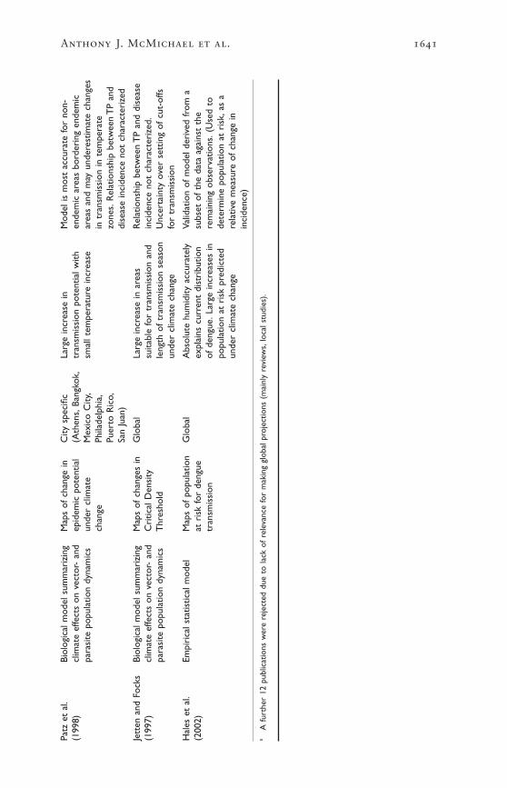
Anthony J. McMichael et al. 1641
Patz
et
al.
Biol
ogic
al m
odel
sum
mar
izin
g M
aps
of c
hang
e in
C
ity s
peci
fic
Larg
e in
crea
se in
M
odel
is m
ost
accu
rate
for
non-
(199
8)cl
imat
e ef
fect
s on
vec
tor-
and
ep
idem
ic p
oten
tial
(Ath
ens,
Bang
kok,
tran
smis
sion
pot
entia
l with
en
dem
ic a
reas
bor
deri
ng e
ndem
ic
para
site
pop
ulat
ion
dyna
mic
sun
der
clim
ate
Mex
ico
City
,sm
all t
empe
ratu
re in
crea
sear
eas
and
may
und
eres
timat
e ch
ange
sch
ange
Phila
delp
hia,
in t
rans
mis
sion
in t
empe
rate
Pu
erto
Ric
o,zo
nes.
Rel
atio
nshi
p be
twee
n T
P an
dSa
n Ju
an)
dise
ase
inci
denc
e no
t ch
arac
teri
zed
Jett
en a
nd F
ocks
Biol
ogic
al m
odel
sum
mar
izin
g M
aps
of c
hang
es in
G
loba
lLa
rge
incr
ease
in a
reas
R
elat
ions
hip
betw
een
TP
and
dise
ase
(199
7)cl
imat
e ef
fect
s on
vec
tor-
and
C
ritic
al D
ensi
ty
suita
ble
for
tran
smis
sion
and
inci
denc
e no
t ch
arac
teri
zed.
para
site
pop
ulat
ion
dyna
mic
sT
hres
hold
leng
th o
f tr
ansm
issi
on s
easo
nU
ncer
tain
ty o
ver
sett
ing
of c
ut-o
ffsun
der
clim
ate
chan
gefo
r tr
ansm
issi
on
Hal
es e
t al
.Em
piri
cal s
tatis
tical
mod
elM
aps
of p
opul
atio
n G
loba
lA
bsol
ute
hum
idity
acc
urat
ely
Valid
atio
n of
mod
el d
eriv
ed f
rom
a(2
002)
at r
isk
for
deng
ue
expl
ains
cur
rent
dis
trib
utio
n su
bset
of
the
data
aga
inst
the
tr
ansm
issi
onof
den
gue.
Larg
e in
crea
ses
in
rem
aini
ng o
bser
vatio
ns.(
Use
d to
popu
latio
n at
ris
k pr
edic
ted
dete
rmin
e po
pula
tion
at r
isk,
as a
un
der
clim
ate
chan
ge
rela
tive
mea
sure
of
chan
ge in
in
cide
nce)
aA
fur
ther
12
publ
icat
ions
wer
e re
ject
ed d
ue t
o la
ck o
f re
leva
nce
for
mak
ing
glob
al p
roje
ctio
ns (
mai
nly
revi
ews,
loca
l stu
dies
).

Appendix referencesAdegbola RA, Demba E, de Veer G, Todd J (1994) Cryptosporidium infection in
Gambian children less than 5 years of age. Journal of Tropical Medicine and Hygiene,97:103–107.
Adkins HJ, Escamilla J, Santiago LT, Ranoa C, Echeverria P, Cross JH (1987) Two-yearsurvey of etiologic agents of diarrheal disease at San Lazaro Hospital, Manila, Repub-lic of the Philippines. Journal of Clinical Microbiology, 25:1143–1147.
Aggarwal P, Sarkar R, Gupta JP, Ahuja S, Ray K, Rai Chowdhuri AN (1983) Currentepidemiological aspects of cholera in Delhi. Journal of Communicable Diseases,15:26–32.
Alberdi JC (1998) Daily mortality in Madrid community, 1986–1992: relationship withmeteorological variables. European Journal of Epidemiology, 14:571–578.
Anjaneyulu G, Banerji SC, Indrayan A (1975) A study of fly density and meteorologi-cal factors in occurrence of diarrhoea in a rural area. Indian Journal of Public Health,19:115–121.
Ansari SA, Springthorpe VS, Sattar SA (1991) Survival and vehicular spread of humanrotaviruses—possible relation to seasonality of outbreaks. Reviews of Infectious Dis-eases, 13:448–461.
Armah GE, Mingle JAA, Dodoo AK et al. (1994) Seasonality of rotavirus infection inGhana. Annals of Tropical Paediatrics, 14:223–229.
Arnell N, Cannell MG, Hulme M et al. (2002) The consequences of CO2 stabilizationfor the impacts of climate change. Climatic Change, 53:413–446
Baarse G (1995) The development of an operational tool for global vulnerability assessment(GVA) update of the number of people at risk due to sea level rise and increased flood-ing probabilities. Ministry of Transport, Public Works and Water Management, TheHague.
Ballester DF, Corella D, Perez-Hoyos S, Saez M, Hervas A (1997) Mortality as a func-tion of temperature. A study in Valencia, Spain, 1991–1993. International Journal ofEpidemiology, 26:551–561.
Beards G, Graham C (1995) Temporal distribution of rotavirus G-serotypes in theWest Midlands region of the United Kingdom, 1983–1994. Journal of Diarrhoeal Dis-eases Research, 13:235–237.
Becker S (1981) Seasonality of deaths in Matlab, Bangladesh. International Journal of Epi-demiology, 10:271–280.
Bishop RF, Masendycz PJ, Bugg HC, Carlin JB, Barnes GL (2001) Epidemiological pat-terns of rotaviruses causing severe gastroenteritis in young children throughout Aus-tralia from 1993 to 1996. Journal of Clinical Microbiology, 39:1085–1091.
Bockemuhl J (1976) Salmonellosis and shigellosis in Togo (West Africa), 1971–1973. I.Carrier rates in the rural population. Tropenmedizin und Parasitologie, 27:112–120.
Booij MJ, (2002) Extreme daily precipitation in Western Europe with climate changeat appropriate spatial scales. International Journal of Climatology, 22:69–85.
Brewster DR, Greenwood BM (1993) Seasonal-variation of pediatric diseases in theGambia, West-Africa. Annals of Tropical Paediatrics, 13:133–146.
1642 Comparative Quantification of Health Risks

Bryan JH, Foley DH, Sutherst RW (1996) Malaria transmission and climate change inAustralia. Medical Journal of Australia, 164:345–347.
Callejas D, Estevez J, Porto-Espinoza L et al. (1999) Effect of climatic factors on theepidemiology of rotavirus infection in children under 5 years of age in the city ofMaracaibo, Venezuela [in Spanish]. Investigacion Clinica, 40:81–94.
Chakravarti A, Broor S, Natarajan R, Setty VS, Mittal SK (1992) Epidemiological andclinical characteristics of acute diarrhoea in children due to human rotavirus. Journalof Tropical Pediatrics, 38:192–193.
Chan PKS, Tam JS, Nelson EAS et al. (1998) Rotavirus infection in Hong Kong: epi-demiology and estimates of disease burden. Epidemiology and Infection, 120:321–325.
Chaudhury A, Nath G, Shukla B, Panda S, Singh TB (1996) Diarrhoea associated withCandida spp.: incidence and seasonal variation. Journal of Diarrhoeal Diseases Research,14:110–112.
Checkley W, Epstein LD, Gilman RH et al. (2000) Effect of El Niño and ambient tem-perature on hospital admissions for diarrhoeal diseases in Peruvian children. TheLancet, 355:442–450.
Conteas CN, Berlin OG, Lariviere MJ et al. (1998) Examination of the prevalence andseasonal variation of intestinal microsporidiosis in the stools of persons with chronicdiarrhea and human immunodeficiency virus infection. American Journal of TropicalMedicine and Hygiene, 58:559–561.
Cook SM, Glass RI, LeBaron CW, Ho MS (1990) Global seasonality of rotavirus infec-tions. Bulletin of the World Health Organization, 68:171–177.
Cunliffe NA, Kilgore PE, Bresee JS et al. (1998) Epidemiology of rotavirus diarrhoeain Africa: a review to assess the need for rotavirus immunization. Bulletin of the WorldHealth Organization, 76:525–537.
da Rosa e Silva ML, Naveca FG, Pires de Carvalho I (2001) Epidemiological aspects ofrotavirus infections in Minas Gerais, Brazil. Brazilian Journal of Infectious Diseases,5:215–222.
Dean AG, Jones TC (1972) Seasonal gastroenteritis and malabsorption at an Ameri-can military base in the Philippines. I. Clinical and epidemiologic investigations ofthe acute illness. American Journal of Epidemiology, 95:111–127.
Dessai SR (2003) Heat stress and mortality in Lisbon. Part II. An assessment of thepotential impacts of climate change. International Journal of Biometeorology, 48:37–44.
Douglas AS, Kurien A (1997) Seasonality and other epidemiological features ofhaemolytic uraemic syndrome and E-coli O157 isolates in Scotland. Scottish MedicalJournal, 42:166–171.
Duncan K, Guidotti TL, Cheng K et al. (1997) The Canadian Country study: impactsand adaptation, Health Sector. In: The Canadian Country study: climate impacts andadaptation, National Sectoral Volume VII. Environment Canada. Toronto.
Eberhard ML, Nace EK, Freeman AR, Streit TG, Da Silva AJ, Lammie PJ (1999)Cyclospora cayetanensis infections in Haiti: a common occurrence in the absence ofwatery diarrhea. American Journal of Tropical Medicine and Hygiene, 60:584–586.
Fischer G, Frohberg K, Parry ML, Rosenzweig C (1994) Climate-change and worldfood-supply, demand and trade—who benefits, who loses. Global EnvironmentalChange-Human and Policy Dimensions, 4:7–23.
Anthony J. McMichael et al. 1643

Fowler AM, Hennessy KJ (1995) Potential impacts of global warming on the frequencyand magnitude of heavy precipitation. Natural Hazards, 11:283–303.
Fujita Y (1990) Rotavirus infection—clinical symptoms and influence of climate [inJapanese]. Kansenshogaku Zasshi, 64:1255–1263.
Gouveia N, Hajat S, Armstrong B (2003) Socio-economic differentials in the temper-ature-mortality relationship in Sao Paulo, Brazil. International Journal of Epidemiology,32:390–397.
Guest CS, Willson K, Woodward AJ et al. (1999) Climate and mortality in Australia.Retrospective study, 1979–1990, and predicted impacts in five major cities in 2030.Climate Research, 13:1–15.
Hales S, de Wet N, Maindonald J, Woodward A (2002) Potential effect of populationand climate changes on global distribution of dengue fever: an empirical model. TheLancet, 360:830–834.
Henry FJ, Bartholomew RK (1990) Epidemiology and transmission of rotavirus infec-tions and diarrhoea in St. Lucia,West Indies. West Indian Medical Journal, 39:205–212.
Hirschl AM, Lior H, Wolf D et al. (1987) Occurrence, serotypes and biotypes of ther-mophilic Campylobacters isolated in Vienna. Zentralblatt für Bakteriologie, Mikrobiolo-gie, und Hygiene, Serie A, 266:94–103.
Hoge CW, Shlim DR, Echeverria P, Rajah R, Herrmann JE, Cross JH (1996) Epidemi-ology of diarrhea among expatriate residents living in a highly endemic environment.Journal of the American Medical Association, 275:533–538.
Hoozemans FMJ, Marchand M, Pennekamp HA (1993) A global vulnerability analysis: vul-nerability assessment for population, coastal wetlands and rice production on a global scale.2nd edn. Delft Hydraulics, Delft.
Ijaz MK, Sattar SA, Johnson-Lussenburg CM, Springthorpe VS, Nair RC (1985) Effectof relative humidity, atmospheric temperature, and suspending medium on the air-borne survival of human rotavirus. Canadian Journal of Microbiology, 31:681–685.
ISOTHURM (forthcoming) ISOTHURM Study Group: international study of temper-ature and heat-waves on urban mortality in low and middle income countries. TheLancet,
Jetten TH, Focks DA (1997) Potential changes in the distribution of dengue transmis-sion under climate warming. American Journal of Tropical Medicine and Hygiene,57:285–287.
Jetten TH, Martens WJM, Takken W (1996) Model simulations to estimate malaria riskunder climate change. Journal of Medical Entomology, 33:361–371.
Jin SX, Kilgore PE, Holman RC, Clarke MJ, Gangarosa EJ, Glass RI (1996) Trends inhospitalizations for diarrhea in United States children from 1974 through 1992: esti-mates of the morbidity associated with rotavirus. Pediatric Infectious Disease Journal,15:397–404.
Jones PD, Reid PA (2001) Assessing future changes in extreme precipitation overBritain using regional climate model integrations. International Journal of Climatology,21:1337–1356.
Kalkstein LS, Greene JS (1997) An evaluation of climate/mortality relationships in largeUS cities and the possible impacts of a climate change. Environmental Health Per-spectives, 105:84–93.
1644 Comparative Quantification of Health Risks

Kalkstein LS, Smoyer KE (1993) The impact of climate change on human health: someinternational implications. Experientia, 49:969–979.
Konno T, Suzuki H, Katsushima N et al. (1983) Influence of temperature and relativehumidity on human rotavirus infection in Japan. Journal of Infectious Diseases,147:125–128.
Kunst A, Looman C, Mackenbach J (1993) Outdoor air temperature and mortality inthe Netherlands—a time series analysis. American Journal of Epidemiology,137:331–341.
Langford IH, Bentham G (1995) The potential effects of climate-change on winter mor-tality in England and Wales. International Journal of Biometeorology, 38:141–147.
Laursen E, Mygind O, Rasmussen B, Ronne T (1994) Gastroenteritis: a waterborneoutbreak affecting 1600 people in a small Danish town. Journal of Epidemiology andCommunity Health, 48:453–458.
LeBaron CW, Lew J, Glass RI, Weber JM, Ruiz-Palacios GM (1990) Annual rotavirusepidemic patterns in North America. Results of a 5-year retrospective survey of 88centers in Canada, Mexico, and the United States. Rotavirus Study Group. Journalof the American Medical Association, 264:983–988.
Lindsay SW, Martens WJM (1998) Malaria in the African highlands: past, present andfuture. Bulletin of the World Health Organization, 76:33–45.
Ling JM, Cheng AF (1993) Infectious diarrhea in Hong-Kong. Journal of Tropical Medi-cine and Hygiene, 96:107–112.
Malakooti MA, Alaii J, Shanks GD, Phillips-Howard PA (1997) Epidemic dysentery inwestern Kenya. Transactions of the Royal Society of Tropical Medicine and Hygiene,91:541–543.
Martens P (1997) Health impacts of climate change and ozone depletion: an eco-epidemi-ological modelling approach. Maastricht University, Maastricht.
Martens W (1998a) Climate change, thermal stress and mortality changes. SocialScience Medicine, 46:331–334.
Martens WJ, Jetten TH, Rotmans J, Niessen LW (1995a) Climate change and vector-borne diseases: a global modelling perspective. Global Environmental Change,5:195–209.
Martens WJ, Niessen LW, Rotmans J, Jetten TH, McMichael AJ (1995b) Potential impactof global climate change on malaria risk. Environmental Health Perspectives,103:458–464.
Martens WJM, Jetten TH, Focks DA (1997) Sensitivity of malaria, schistosomiasis anddengue to global warming. Climatic Change, 35:145–156.
Martens P, Kovats RS, Nijhof S et al. (1999) Climate change and future populations atrisk of malaria. Global Environmental Change—Human and Policy Dimensions,9:S89–S107.
Martin PH, Lefebvre MG (1995) Malaria and climate—sensitivity of malaria potentialtransmission to climate. Ambio, 24:200–207.
Matsuoka Y, Kai K (1994) An estimation of climatic change effects on malaria. Journalof Global Environment Engineering, 1:1–15.
Anthony J. McMichael et al. 1645

McMichael AJ, Kovats S, Martens P et al. (2000b) Climate change and human health: finalreport to the Department of Environment,Transport and the Regions. London School ofHygiene and Tropical Medicine/ICIS, London/Maastricht.
Merlin M, Roure C, Kollo B et al. (1986) Evaluation of morbidity, mortality and ther-apeutic procedures in diarrheal diseases of young children in Cameroon. MédecineTropicale (Marseilles), 46:355–357.
Milly PCD, Wetherald RT, Dunne KA, Delworth TL (2002) Increasing risk of greatfloods in a changing climate. Nature, 415:514–517.
Muhuri PK (1996) Estimating seasonality effects on child mortality in Matlab,Bangladesh. Demography, 33:98–110.
Musa HA, Shears P, Kafi S, Elsabag SK (1999) Water quality and public health in north-ern Sudan: a study of rural and peri-urban communities. Journal of Applied Microbi-ology, 87:676–682.
Nchito M, Kelly P, Sianongo S et al. (1998) Cryptosporidiosis in urban Zambian chil-dren: an analysis of risk factors. American Journal of Tropical Medicine and Hygiene,59:435–437.
Nicholls RJ, Mimura N (1998) Regional issues raised by sea level rise and their policyimplications. Climate Research, 11:5–18.
Nicholls RJ, Hoozemans FMJ, Marchand M (1999) Increasing flood risk and wetlandlosses due to global sea—level rise: regional and global analyses. Global EnvironmentalChange-Human and Policy Dimensions, 9:S69–S87.
Palmer TN, Ralsanen J (2002) Quantifying the risk of extreme seasonal precipitationevents in a changing climate. Nature, 415:512–514.
Parashar UD, Chung MA, Holman RC, Ryder RW, Hadler JL, Glass RI (1999) Use ofstate hospital discharge data to assess the morbidity from rotavirus diarrhea andto monitor the impact of a rotavirus immunization program: a pilot study in Con-necticut. Pediatrics, 104:489–494.
Parashar UD, Holman RC, Bresee JS et al. (1998a) Epidemiology of diarrheal diseaseamong children enrolled in four west coast health maintenance organizations. Pedi-atric Infectious Disease Journal, 17:605–611.
Parashar UD, Holman RC, Clarke MJ, Bresee JS, Glass RI (1998b) Hospitalizationsassociated with rotavirus diarrhea in the United States, 1993 through 1995: sur-veillance based on the new ICD-9-CM rotavirus-specific diagnostic code. Journal ofInfectious Diseases, 177:13–17.
Parry M, Rosenzweig C, Iglesias A, Fischer G, Livermore M. (1999) Climate changeand world food security: a new assessment. Global Environmental Change-Human andPolicy Dimensions, 9:S51–S67.
Parry ML,Arnell NW, McMichael A et al. (2001) Millions at risk: defining critical climatechange threats and targets. Global Environmental Change, 11:181–183.
Patz JA, Martens WJM, Focks DA, Jetten TH (1998) Dengue fever epidemic potentialas projected by general circulation models of global climate change. EnvironmentalHealth Perspectives, 106:147–153.
Pazzaglia G, Bourgeois AL, Araby I et al. (1993) Campylobacter-associated diarrhea inEgyptian infants—epidemiology and clinical manifestations of disease and high-fre-quency of concomitant infections. Journal of Diarrhoeal Diseases Research, 11:6–13.
1646 Comparative Quantification of Health Risks

Pinfold JV, Horan NJ, Mara DD (1991) Seasonal effects on the reported incidence ofacute diarrhoeal disease in northeast Thailand. International Journal of Epidemiology,20:777–786.
Purohit SG, Kelkar SD, Simha V (1998) Time series analysis of patients with rotavirusdiarrhoea in Pune, India. Journal of Diarrhoeal Diseases Research, 16:74–83.
Qiao HP, Nilsson M, Abreu ER et al. (1999) Viral diarrhea in children in Beijing, China.Journal of Medical Virology, 57:390–396.
Ram S, Khurana S, Khurana SB, Sharma S, Vadehra DV (1990a) Seasonal fluctuationsin the occurrence of enteroinvasive Escherichia coli diarrhoea. Indian Journal ofMedical Research, 91:258–262.
Ram S, Khurana S, Khurana SB, Sharma S, Vadehra DV, Broor S (1990b) Bioecologi-cal factors and rotavirus diarrhoea. Indian Journal of Medical Research, 91:167–170.
Reyes M, Hedlund KO, Lorenzana I, Ehrnst A (1996) Respiratory infection and iatro-genic diarrhea in Honduras and El Salvador during the 1991–1992 season. AmericanJournal of Tropical Medicine and Hygiene, 54:260–264.
Robins-Browne RM (1984) Seasonal and racial incidence of infantile gastroenteritis inSouth Africa. American Journal of Epidemiology, 119:350–355.
Rogers DJ (1996) Regional impacts of climate change; changes in disease vector dis-tributions. In: Climate change and Southern Africa: an exploration of some potentialimpacts and implications in the SADC region. Hulme M, ed. University of East Anglia,Norwich.
Rogers DJ, Randolph SE (2000) The global spread of malaria in a future, warmer world.Science, 289:1763–1766.
Rosenzweig C, Parry ML (1994) Potential impact of climate-change on world food-supply. Nature, 367:133–138.
Rousham EK, Mascietaylor CGN (1995) Seasonality and child morbidity in ruralBangladesh. American Journal of Human Biology, 7:369–379.
Rytlewska M, Bako W, Ratajczak B et al. (2000) Epidemiological and clinical charac-teristics of rotaviral diarrhoea in children from Gdansk, Gdynia and Sopot. MedicalScience Monitor 6:117–122.
Saidi SM, Iijima Y, Sang WK et al. (1997) Epidemiological study on infectious diarrhealdiseases in children in a coastal rural area of Kenya. Microbiology and Immunology,41:773–778.
Sallon S, el Showwa R, el Masri M, Khalil, M, Blundell N, Hart CA (1991) Cryp-tosporidiosis in children in Gaza. Annals of Tropical Paediatrics, 11:277–281.
Sawchuk LA (1993) Societal and ecological determinants of urban health: a case studyof pre-reproductive mortality in 19th century Gibraltar. Social Science and Medicine,36:875–892.
Sethi SK, Al-Nakib W, Khuffash FA, Majeed HA (1984) Acute diarrhoea and rotavirusinfections in young children in Kuwait. Annals of Tropical Paediatrics, 4:117–121.
Shahid NS, Rahman AS, Sanyal SC (1987) Cryptosporidium as a pathogen for diar-rhoea in Bangladesh. Tropical and Geographical Medicine, 39:265–270.
Anthony J. McMichael et al. 1647
Shaikh K, Wojtyniak B, Mostafa G, Khan MU (1990) Pattern of diarrheal deaths during1966–1987 in a demographic surveillance area in rural Bangladesh. Journal of Diar-rhoeal Diseases Research, 8:147–154.
Shkarin VV, Ouchfoun A, Minaev VI, Naceur D (1983) Epidemiology of bacillary dysen-tery in Algeria. II. The seasonality of dysentery. Zhurnal Mikrobiologii, Epidemiologii iImmunobiologii, 53–58.
Singh RB, Hales S, de Wet N, Raj R, Hearnden M, Weinstein P (2001) The influenceof climate variation and change on diarrheal disease in the Pacific Islands. Environ-mental Health Perspectives, 109:155–159.
Sorvillo F, Beall G,Turner PA et al. (1998) Seasonality and factors associated with cryp-tosporidiosis among individuals with HIV infection. Epidemiology and Infection,121:197–204.
Stewien KE, Dacunha LCF, Alvim AD et al. (1991) Rotavirus associated diarrhea duringinfancy in the city of S Luis (Ma), Brazil—a 2-year longitudinal-study. Revista do Insti-tuto de Medicina Tropical de São Paulo, 33:459–464.
Stintzing G, Back E, Tufvesson B, Johnsson T, Wadstrom T, Habte D (1981) Seasonalfluctuations in the occurrence of entero-toxigenic bacteria and rotavirus in pedi-atric diarrhea in Addis-Ababa. Bulletin of the World Health Organization, 59:67–73.
Sutra S, Srisontrisuk S, Panpurk W et al. (1990) The pattern of diarrhea in children inKhon Kaen, northeastern Thailand: I. The incidence and seasonal variation of diar-rhea. Southeast Asian Journal of Tropical Medicine and Public Health, 21:586–593.
Tanser FC, Sharp B, Le Sueur D (2003) Potential effect of climate change on malariatransmission in Africa. The Lancet, 362:1792–1798.
Tsukamoto T, Kinoshita Y, Shimada T, Sakazaki R (1978) Two epidemics of diarrhoealdisease possibly caused by Plesiomonas shigelloides. Journal of Hygiene, 80:275–280.
Tswana SA, Jorgensen PH, Halliwell RW, Kapaata R, Moyo SR (1990) The incidenceof rotavirus infection in children from 2 selected study areas in Zimbabwe. CentralAfrican Journal of Medicine, 36:241–246.
Utsalo SJ, Eko FO, Antia-Obong OE (1991) Cholera and Vibrio parahaemolyticus diar-rhoea endemicity in Calabar, Nigeria. West African Journal of Medicine, 10:175–180.
Van den Broeck J, Eeckels R, Devlieger H (1993) Child morbidity patterns in two trop-ical seasons and associated mortality rates. International Journal of Epidemiology,22:1104–1110.
Varoli O, Gatti M, Piscolla F (1989) A one-year study on thermophilic campylobactersisolated from fecal specimens. Microbiologica, 12:263–265.
Vlasov VI, Zamotin BA, Burykh VM (1983) Method for the short-term prognosis ofannual morbidity indices in Sonne-type dysentery. Zhurnal Mikrobiologii, Epidemiologiii Immunobiologii, 53–56.
Warrick RA, Barrow EM (1991) Climate change scenarios for the UK. Transactions ofthe Institute of British Geographers, 16:387–399.
Wilcox MH, Cook AM, Eley A, Spencer RC (1992) Aeromonas spp. as a potential causeof diarrhoea in children. Journal of Clinical Pathology, 45:959–963.
Williams EH, Hayes RJ, Smith PG (1986) Admissions to a rural hospital in the WestNile District of Uganda over a 27 year period. Journal of Tropical Medicine and Hygiene,89:193–211.
1648 Comparative Quantification of Health Risks

Wuhib T, Silva TM, Newman RD et al. (1994) Cryptosporidial and micro-sporidial infec-tions in human immunodeficiency virus-infected patients in northeastern Brazil.Journal of Infectious Diseases, 170:494–497.
Yang CR, Meng ZD, Wang X, Li YL, Zhang YX, Zhao QP (1990) Diarrhea surveillancein children aged under 5 years in a rural area of Hebei Province, China. Journal ofDiarrhoeal Diseases Research, 8:155–159.
Anthony J. McMichael et al. 1649
