18

CHAPTER 2

RESEARCH DESIGN

2.1 INTRODUCTION

As it’s said before, the most aim of this research is to show that if the advertising

costs have long benefits, it must be shown as an intangible asset in financial

statements and in their useful lives, they must amortize. But if they have not

benefited for more than one period, they must be show as expenses in financial

statements. Also the selection of each one of this policy can have meaningful

effects on reporting of profits. To exist of these hesitation caused many scientist

have done research in this field that will be explained in chapter three. In this

chapter it will be tried to explain about research design as a through.

2.2 DEFINING THE RESEARCH PROBLEM:

As we know, the research problem undertaken for study must be carefully

selected(1)

. Help may be taken from a research guide in this connection. A problem

must spring from the researcher’s mind like a plant springing from its own seed.

However, the following points to take into consideration :

1. The subject which is overdone is not be normally chosen, if it will be a difficult

task to throw any new light in such a case.

1. Kothary, C.R. “Research Methodology Methods & Techniques” News Age

International Publishers, second edition, 2004, P. 25.

19

2. Controversial subject is not the choice of an average.

3. Too narrow or too vague problems are avoided.

4. The subject selected for research is familiar and feasible so that the related

research material or sources of research are within one’s reach.

5. The importance of the subject, the qualifications and the training of a researcher,

the costs involved, the time factor are consider in selecting the problem.

In other words, before the final selection of a the problem, researcher asked himself

the following questions :

i) Whether he is well equipped in terms of his background to carry out the research?

ii) Whether the study falls within the budget he can afford?

iii) Whether the necessary cooperation can be obtained from those who must

participate in research as subject.

By answering to all these questions, I become sure so for as the practicability of the

study is concerned.

6. The selection of a problem is preceded by a preliminary study.

The purpose of research is to discover answers to questions through the

application of scientific procedures. The main aim of research is to find out the truth

which is hidden and which has not been discovered as yet. A research design is the

arrangement of conditions for collection and analysis of data in a manner that aims to

combine relevance to the research purpose with economy in procedure. Some points

that are attended for defining the problem are :

a) There must be an individual or a group which has some difficulty or the problem.

b) There must be some adjectives to be attained at.

20

c) There must be at least two means available to a researcher for if he has no choice

of means, he cannot have a problem.

d) There must remain some doubt in the mind of a researcher with regard to the

selection of alternatives. This means that research must answer the question

concerning the relative efficiency of the possible alternatives.

e) There must be some environments to which the difficulty pertains.

In the research it is tried to answer to the question that whether the advertising

affects on the companies’ sales or not? If so, then we can say that the effect of

advertising relates to the same period of advertising or would affect on the sales in

the future? And thus form point of accounting how can we treat such advertising

costs?

2.3 OBJECTIVES OF THE STUDY

i) To study the importance of advertising

ii) To study the effect of advertising costs on the sales of companies.

iii)To study the effect of advertising costs on the net incomes.

iv)To study a suitable method for accounting of advertising costs.

v) To study the rate of amortization for advertising costs and compare

it with appropriate method.

2.4 HYPOTHESES FORMATION :

Hypothesis is usually considered as the principal instrument in research. Its main

function is to suggest new experiments and observations. In fact, many experiments

are carried out with the deliberate object of testing hypothesis. Ordinarily, when one

talks about hypothesis, one simply means a mere assumption or some supposition to

21

be proved or disproved. But for a researcher hypothesis is a formal question that he

intends to resolve.

As it was explained, the most importance aspect of any business is selling the

product or services. Without sales, no business can exist for very long. All sales

begin with some form of advertising. In fact, management advertises for one reason;

to increase sales(1)

. Therefore, advertising can only be evaluated meaningfully for

management ( not the agent) by determining whether or not it does increase sales and

by how much.(( The methodological problem is this : given a set of conditions,

which when they occur after event A (advertising), produce a sale, can we determine

the effect of A on sales when we don’t control these other conditions)).(2)

This statement appear to reduce the two possibilities into only one, the objective

is to generate additional sales. According to the present accounting model, if the

response of demand to advertising is delayed beyond the current period, advertising

expenditures, which are incurred currently, would be expected to generate revenues

in the future and should therefore be deferred until such time when the stimulated

revenues are deemed red gal. Then the main objective of this research is to test the

following statements of hypotheses:

I) Advertising costs, for food industry, have important effect on the sales of

next periods, and then they must not become as a periodical expense.

1. Rao, J. A. “Quantitative Theories in Advertising”, J, Wiley, 1970 P. 7.

2. Ibid

22

II) The use of suitable methods of amortization of advertising costs can have

important effects on the net income of each period.

According to the explanations of above, the effect of advertising on sales of food

industry will be tested.

2.5 SCOPE FOR THE STUDY

Data were gathered(1)

on annual revenues and annual costs of all promotional

efforts as issued by CMIE(2)

for each group of food industry for 7 years from 1998

through 2004. Because detailed data for each firm was not available, the firms were

divided into 9 groups and each group was tested; and because observations for each

group were small, all the 9 groups were tested by treating them as a single group(3)

.

These were altogether 1512 companies divided into 9 groups as follows:

1. Food Products (475) 2. Food and Beverage (527)

1. All items in any field of inquiry constitute a ‘Universe’ or ‘Population’. A

complete enumeration of all items in the population in known as a census

inquiry. It can be presumed that in such an inquiry, when all items are covered,

no element of chance is left and highest accuracy is obtained. In this research we

used census surveys instead of sample surveys.

2. Centre for Monitoring Indian Economy Pvt. Ltd.

3. In estimating of the data, line series and cross-sectional data will pooled as a

group and with the use of dummy variables, each groups will be allowed to have

individual intercepts in order to capture some of them unique characteristics.

Padding time series and cross-sectional data is necessary in order to reduce the

multicollinearity between explanatory variables and in order to increase the

sample size such the properties of linear models with lagged dependent variables

are still unknown for small samples

23

3. Dairy product (20) 4. Tea and Coffee (125)

5. Sugar (68) 6. Vegetable Oils and Products (92).

7. Vanaspati (19) 8. Soya been Products (16)

9. Other Food Product (170)

2.6 RESEARCH METHODOLOGY

2.6.1 Type of the research

Research methodology is a way to systematically solve research problems. It

may be understood as a science of studying how research is done scientifically. The

basic type of this research is quantitative. Quantitative research is based on the

measurement of quantity or amount. It is applicable to phenomena that can be

expressed in terms of quantity. For testing of the collected data, Koyck distributed

lag model was used. The nature of the problem and the structure of the lag models

required using at least two variables: lag dependent variable (sales) and advertising

costs (independent variable). These two variables were common for four of the

models used.

2.6.2 Collection of data

The researcher used the following methodology for data collection for the study:

i) Primary data - Primary data for studying were collected by following means:

a) Stock market visit; and

b) b)CMIE visit.

ii) Secondary data – Secondary data for studying were collected by the

following means:

24

a) Books;

b) Journals;

c) Financial statements reports of food industry; and

d) Govt. publications and stock market publications.

2.7 TEST OF HYPOTHESIS

The literature on advertising effectiveness has been largely based on the

assumption of decaying cumulative effects. The Koyck distributed lag model has

been used with reasonable success in marketing research to provide a method for the

measurement of the cumulative effects of advertising(1)

. The distributed lag and

regression models will be explained completely.

The simple linear model(2)

: The correlation coefficient my indicate that two

variables are associated with on another, but in does not give any idea of the kind of

relationship involved. It must be stated that one would not expect to find an exact

relationship between any two economic variables, unless it is true as a matter of

definition. In statistical analysis, however, one generally acknowledges the fact that

the relationship is not exact by explicitly including in it a random factor known as

the disturbance term. The simplest regression model is :

(2-7-1) Y= +X + u

Y, described as the dependent variable, has two components :

1. See Johnston, 1972, pp. 297-300; Palda, 1964; Bass and Clark, 1972, and

Beckwith, 1972, etc.

2. Dougherty, CH. “Introduction to Econometrics” Oxford University Press, 1992

p.53.

25

1. the nonrandom component +x , x being described as the explanatory (or

independent) variable and the fixed quantities and as the parameters

of the equation, and

2. the disturbance term, u.

Multiple Regression Model: Multiple regression analysis allows one to discriminate

between the affects of the explanatory variables, making allowance for the fact that

they may be correlated. The regression coefficient of each or variable provides on

estimate of its influence on Y, controlling for the effects of all the other X variables.

This can be demonstrated in two ways. One is to show that the estimates are

unbiased, if the model is correctly specified, and the Gauss-Maker conditions are

fulfilled. We shall do this in the next section for the case in which there are only two

explanatory variables. A second method is to run a simple regression of Y against

one of the explanatory variables, having first purged the latter of its ability to act as a

proxy for any of the other explanatory variables, and to show that the estimate of its

coefficient, thus obtained is exactly the same as its multiple regression coefficient .

The multiple regression model is :

(2-7-2) Y= + 1X1 + 2X2 +u

Suppose, for the time being, that 1 and 2 are both positive and that X1 and X2

are positively correlated. What would happen if you can a straight forward simple

regression of Y against X1? Well, as X1 increase, (1) Y will tend to increase, because

1 is positive; (2) X2 will tend to increase, because X1 and X2 are positively

correlated, and (3) Y will receive a boost because of the increase in X2 and the fact

26

that 2 is positive. In other words, variations in Y will exaggerate the apparent

influence of X1 because in part they will be due to associated variations in X2.

General regression model for several independent variables is

(2-7-3) Y= + 1X1 + 2X2 +….. +k Xk + u.

2.8 AUTOREGRESSIVE AND DISTRIBUTED LAG MODELS (1)

In regression analysis involving time series data, if the regression model

includes not only the current but also the lagged (past) values of the explanatory

variables (the X’s), it is called a distributed-lag model. If the model includes one or

more lagged values of the dependent variable among its explanatory variables, it is

called an autoregressive model. Thus:

(2-8-1) Yt = + 0Xt +1Xt-1 +2Xt-2+ut

represents a distributed – lag model, whereas:

(2-8-2) Yt = + Xt+ Yt-1 + ut

is an example of an autoregressive model. The latter are also known as dynamic

model since they portray the time path of the dependent variable in relation to its

past value(s).

Autoregressive and distributed-lag models are used extensively in econometric

analysis, and in this chapter we take a close look at such model with a view to

finding out the following:

1. What is the role of lags in economics?

2. What are the reasons for the lags?

1. Gujerathi, D. N. “Basic Econometrics” forth Edition, 2003, P. 384.

27

3. Is there any theoretical justification for the commonly used lagged models in

empirical econometrics?

4. What is the relationship, if any, between autoregressive and distributed-lag

models? Can one be derived from the other?

5. What are some of the statistical problems involved in estimating such models?

6. Does a lead-lag relationship between variables imply causally? If so, how does

one measure it?

2.8.1 THE ROLE OF “TIME,” OR “LAG” IN ECONOMICS

In economics the dependence of a variable Y (the dependent variable) on another

variable(s) X (the explanatory variable) is rarely instantaneous. Very often, Y

responds to X with a lapse of time. Such a lapse of time is called a lag. To illustrate

the nature of the lag, we consider several examples.

Example 1 : The Consumption Function. Suppose a person receive a salary

increase of $2000 in annual pay, and suppose that this is a “permanent” increase in

the sense that the increase in salary is maintained. What will be the effect of this

increase in income on the person’s annual consumption expenditure?

Following such a gain in income, people usually do not rush to spend all the

increase immediately. Thus, our recipient may decide to increase consumption

expenditure by $800 in the first year following the salary increase in income, by

another $600 in the next year, and by another $ 400 in the following year, saving the

remainder. By the end of the third year, the person’s annual consumption

28

expenditure will be increased by $1800. We can thus write the consumption

functions as:

(2-8-3) Yt = Constant + 0.4Xt + 0.3Xt-1 + 0.2X t-2 + ut

Where Y is consumption expenditure and X is income.

Equation (2-8-3) shows that the effect of an increase in income of $ 2000 is

spread, or distributed, over a period of three years. Models such as (2-8-3) are

therefore called distributed-lag models because the effect of a given cause (income)

is spread over a number of time periods. Geometrically, the distributed-lag model (2-

8-3) is shown in Fig. 3.1, or alternative, in Fig. 3.2.

More generally we may write

(2-8-4 ) Yt = + 0Xt + 1Xt-1 + 2 Xt-2 + …… + k Xt-k + ut

which is a distributed-lag model with a finite lag of k time periods. The coefficient 0

is known as the short-run, or impact, multiplier because it gives the change in the

mean value of Y following a unit change in X in the same time period. If the change

in (the mean value of) Y in the next period, (0+1+2) in the following period, and

so on. These partial sums are called interim, or intermediate, multipliers. Finally,

after k periods we obtain

k

(2-8-5) i = 0 + 1 + 2 + …… + k =

i-0

which is known as the long-run, or total, distributed-lag multiplier, provided the

sum exists (to be discussed elsewhere)if we define

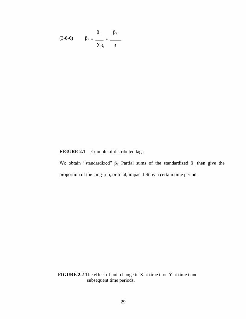
29

i i

(3-8-6) i = _____ = _______

i

FIGURE 2.1 Example of distributed lags

We obtain “standardized” i. Partial sums of the standardized i then give the

proportion of the long-run, or total, impact felt by a certain time period.

FIGURE 2.2 The effect of unit change in X at time t on Y at time t and

subsequent time periods.

30

Returning to the consumption regression (2.8.3), we see that the short run

multiplier, which is nothing but the short-run marginal propensity to consume

(MPC), is, 0.4 whereas the long-run multiplier, which is the long-run marginal

propensity to consume (MPC) is, 0.4, whereas the long-run multiplier, which is the

long-run marginal propensity to consume, is 0.4 + 0.3 + 0.2 = 0.9. That is, following

a $ 1 increase in income, the consumer will increase his or her level of consumption

by about 40 cents in the year of increase, by another 30 cents in the next year, and by

yet another 20 cents in the following year. The long-run impact of an increase of $1

in income is thus 90 cents. If we divide each i by 0.9, we obtain, respectively 0.44,

0.33, and 0.23, which indicate that 44 percent of the total impact of a unit change in

X on Y is felt immediately, 77 percent after one year, and 100 percent by the end of

the second year.

Example 2 : Creation of bank money (demand deposits). Suppose the Federal

Reserve System pours $1000 of new money into the banking system by buying

government securities. What will be the total amount of bank money, or demand

deposits, that will be generated ultimately?

Following the fractional reserve systems, if the assume that the law requires banks

to keep a 20 percent reserve backing for the deposits they create, then by the well-

known multiplier process the total amount of demand deposit that will be generated

will be equal to $1000 {1/(1-08)} = $ 5000. Of course, $ 5000 in demand deposits

will be not created overnight. The process takes time, which can be shown

schematically in Fig. 2.3

31

FIGURE 2.3 Cumulative expansion in bank deposits(initial reserve $1000 and 20

percent reserve requirement).

Example 3 : Link between money and prices. According to the monetarists,

inflation is essentially a monetary phenomenon in the sense that a continuous

increase in the general price level is due to the rate of expansion in money supply far

in excess of the amount of money actually demanded by the economic units. Of

course, this link between inflation and changes in money supply is not instantaneous.

Studies have shown that the lag between the two is anywhere from 3 to about 20

quarters. The results of one such study are shown in Table 3.1, where we see the

effect of a 1 percent change in the M1B money supply (= currency + Checkable

deposit at financial institutions) is felt over a period of 20 quarters. The long-run

impact of a 1 percent change in the money supply on inflation is about 1(= mi),

which is statistically significant, whereas the short-run impact is about 0.04, which is

not significant, although the intermediate multiplies seem to be generally significant.

32

Incidentally, note that since P and M are both in percent forms, the mi (i in our usual

notation) give the elasticity of P with respect to M, that is, the percent response of prices to a

1 percent increase in the money supply. Thus, m0 = 0.041 means that for a 1 percent increase

in the money supply the short-run elasticity of prices is about 0.04 percent. The long-term

elasticity is 1.03 percent, implying that in the long run a 1 percent increase in the money

supply is reflected by just about the same percentage increase in the prices. In short, a 1

percent increase in the money supply is accompanied in the long run by a 1 percent increase

in the inflation rate.

Example 4. Lag between R & D expenditure and productivity. The decision to invest in

research and development (R & D) expenditure and its ultimate payoff in terms of increased

productivity involve considerable lag, actually several lags, such as, “…. the lag between the

investment of funds and the time inventions. actually begin to appear, the lag between

Table 2.1 : Estimate of money-price equation ; Original specification

33

the invention of an idea or device and its development up to a commercially

applicable stage, and the lag which is introduced by the process of diffusion : it takes

time before all the old machines are replaced by the better new ones ”

The preceding examples are only a sample of the use of lag in economics.

Undoubtedly, the reader can produce several examples from his or her own

experience.

2.8.2 THE REASONS FOR LAGS

There are three main reasons for logs occur.

1. Psychological reasons. As a results of the force of habit (inertia), people do not

change their consumption habits immediately following a price decrease or an

income increase perhaps because the process of change may involve some

immediate disutility. Thus, those who become instant millionaires by winning

lotteries may not change the lifestyles to which they were accustomed for a long

time because they may not know how to react to such a windfall gain

immediately. Of course, given reasonable time, they may learn to live with

their newly acquired fortune. Also, people may not know whether a change is

“permanent” or “transitory”. Thus, my reaction to an increase in my income will

depend on whether or not the increase is permanent. If it is only a nonrecurring

increase and in succeeding periods my income returns to its previous level, I

may save the entire increase, whereas someone else in my position might decide

to “live it up”.

34

2. Technological reasons. Suppose the price of capital relative to labor declines,

making substitution of capital for labor economically feasible. Of course,

addition of capital takes time (the gestation period). Moreover, if the drop in

price is expected to be temporary, firms may not rush to substitute capital for

labor, especially if they expect that after the temporary drop the price of capital

may increase beyond its previous level. Sometimes, imperfect knowledge also

accounts for lags. At present the market for personal computers is glutted with

all kinds of computer with varying features and prices. Moreover, since their

introduction in the late 1970s, the prices of most personal computers have

dropped dramatically. As a result, prospective consumers for the personal

computer may hesitate to buy until they have had time to look into the features

and prices of all the competing brands. Moreover, they may hesitate to buy in

the expectation of future decline in price or innovations.

3. Institutional reasons. These reasons also contribute to lags. For example,

contractual obligations may prevent firms from switching form one source of

labor or raw material to another. As another example, those who have placed

funds in long-term savings accounts for fixed durations such as one year, three

years, or seven years, are essentially “locked in” even though money market

conditions may be such that higher yields are available elsewhere. Similarly,

employers often give their employees a choice among several health insurance

plans, but once a choice is made, an employee may not switch to another plan

for at least 1 year. Although this may be done for not switch to another plan for

at least 1 year. Although this may be done for administrative convenience, the

employee is locked in for 1 year.

35

For the reasons just discussed, lag occupies a central role in economics. This is

clearly reflected in the short-run-long methodology of economics. It is for this reason

we say that short-run price or income elasticities are generally smaller(in

absolute value) than the corresponding long-run elasticities or that short-run

marginal propensity to consumer is generally smaller than long-run marginal

propensity to consume.

2.9 ESTIMATION OF DISTRIBUTED-LAG MODELS

Granted that distributed-lag models play a highly useful role in economics, how

does one estimate such models? Specifically, suppose we have the following

distributed-lag model in one explanatory variable.

(2-9-1) Yt = + 0Xt + 1Xt-1 + 2Xt-2 + … + ut

where we have not defined the length of the lag, that is, how far back into the past

we want to go. Such a model is called an infinite (lag) model, whereas a model of

the type (2-8-4) is called a finite (lag) distributed-lag model because the length of

the lag k is specified. We shall continue to use (2-9-1) because it is easy to handle

mathematically, as we shall see.

How do we estimate the and ’s of (2-9-1) ? We may adopt two approaches :

(1) ad hoc estimation and (2) a priori restrictions on the ’s by assuming that the ’s

follow some systematic pattern. We shall consider ad hoc estimation in this section.

2.9.1 AD HOC ESTIMATION OF DISTRIBUTED-LAG MODELS

Since the explanatory variable Xt is assumed to be nonstochastic (or at least

uncorrelated with the disturbance term ut) Xt-1, Xt-2, and so on, are nonstochastic, too.

36

Therefore, in principle, the ordinary least squares (OLS) can be applied to (3-8-1).

This is the approach taken by Alt(1)

and Tinbergen(2)

. They suggest that to estimate

(2-8-1) one may proceed sequentially; that is, first regress Yt on Xt, then regress Yt

on Xt and Xt-1, then regress Yt on Xt, Xt-1, and Xt-2, and so on. This sequential

procedure stops when the regression coefficients of the lagged variables start

becoming statistically insignificant and/or the coefficient of at least one of the

variables changes signs from positive to negative or vice versa. Following this

precept, Alt regressed fuel oil consumption Y on new orders X. Based on the

quarterly data for the period 1930-1939, the results were as follows :

Yt = 8.37 + 0.171Xt

Yt = 8.27 + 0.111Xt + 0.064Xt-1

Yt = 8.27 + 0.109Xt + 0.071Xt-1 – 0.055Xt-2

Yt = 8.32 + 0.108Xt +0.063Xt-1 + 0.022Xt-2 – 0.020Xt-3

Alt chose the second regression as the “best” one because in the last two equations

the sign of Xt-2 was not stable and in the last equation the sign of Xt-3 was negative,

which may be difficult to interpret economically. Although seemingly

straightforward, ad hoc estimation suffers from many drawbacks, such as the

following :

1. There is no a priori guides as to what is the maximum length of the lag.

2. As one estimates successive lags, there are fewer degrees of freedom left, making

statistical inference somewhat shaky. Economists are not usually that lucky to

1. F.F.Alt, “Distrbuted Lags “ Econometrica, vol. 10,1942, pp. 113-128.

2. J. Tinbergen, “Long-Term Foreign Trade Elasticities” , Macroeconomica, vol.1,

1949, pp.174-185.

37

have a long statistical inference somewhat shaky. Economists are not usually that

lucky to have a long series of data so that ythey can go on estimating numerous lags.

3. More importantly, in economic time series data, successive values (lags) tend to

be highly correlated; hence multicollinearity rears its ugly head. Multicollinearity

leads to imprecise estimation, that is, the standard errors tend to be large in

relation to the estimated coefficients. As a result, based on the routinely

computed t ratios, we may tend to declare (erroneously), that a lagged

coefficient(s) is statistically insignificant.

4. The sequential search for the lag length opens the researcher to the charge of data

mining. The nominal and true level of significance to test statistical hypotheses

becomes an important issue in such sequential searchers.

In view of the preceding problems, the ad hoc estimation procedure has very little

to recommend it. Clearly, some prior of theoretical considerations must be brought to

bear upon the various ‘s if we are to make headway with the estimation problem.

2.9.2 THE KOYCK APPROACH TO DISTRIBUTED-LAG MODELS

Koyck has proposed an ingenious method of estimation distributed-lag models.

Suppose we start with the infinite lag distributed-lag model (2-9-1). Assuring that the

‘s are all of the same sign, Koyck assumes that they decline geometrically as follows: (1)

(2-9-2) k =0k k=0,1,2,….

Where , such that 0<<1 is known as the rate of decline, or decay, of the distributed lag and

(1-) is known as the speed of adjustment.

1. Sometimes this is also written as k = 0(1-)k k=0,1,….

38

What (2-9-2) postulates is that each successive coefficient is numerically less than each

preceding (this statement follows since <1 ), implying that as one goes back into the

distant past, the effect of that lag on Yt, becomes progressively smaller, a quite plausible

assumption. After all, current and recent past incomes are expected to affect current

consumption expenditure more heavily than income in the distant past. Geometrically, the

Koyck scheme is depicted in Fig. 3.4. As this figure shows, the value of the lag coefficient

k depends, apart from the common 0, on the value of .The closer is to 1, the slower

the rate of decline in k , whereas the closer it is to zero, the more rapid the decline in k .

In the former case, distant past values of X will exert sizable impact on Yt, whereas in the

latter case their influence on Yt will peter out quickly. This pattern can be seen clearly form

the following illustration:

FIGURE 2.4 Koyck scheme(declining geometric distribution).

39

Note these features of the Koyck scheme : (1) By assuming nonnegative values

for , Koyck rules out the ‘s from changing sing; (2) by assuming <1 he gives

lesser weight to the distant ‘s than the current ones; and (3) he ensures that the

sum of the ’s which gives the long-run multiplier, is finite, namely:

(2-9-3) (1)

Yt = + 0Xt + 1Xt-1 + 2Xt-2 + … + ut

As a result of (2-9-2), the infinite lag model (2-9-1) may be written as

(2-9-4) Yt = + 0Xt + 0Xt-1 + 02Xt-2 + … + ut

As it stands, the model is still not amenable to easy estimation since a large (literally

infinite) number of parameters remain to be estimated and the parameter enters in

a highly nonlinear from : Strictly speaking, the method of linear (in a parameter)

regression analysis cannot be applied to such a model. But now Koyck suggests an

ingenious way out. He lags (2-9-4) by one period to obtain.

(2-9-5 ) Yt-1 = + 0Xt-1 + 0Xt-2+ 02Xt-3 + … + ut-1

He then multiples (2-9-5) by to obtain

(2-9-6) Yt-1 = + 0Xt-1 + 02Xt-2+ 0

3Xt-3 + … + ut-1

Subtracting (2-9-6) form (2-9-4), he gets :

1. This is because: k = o (1+ +2+

3+ …..) = o(1/1-)

Since the expression in the parentheses on the right side is an infinite geometric

series whose sum is 1 /(1- ) provided 0 1. In passing, note that if k is

k = o (1- ) / (1- ) = o thus ensuring that the weight (1- )k sum to one.

40

(2-9-7) Yt - Yt-1 = (1-) + 0Xt + (ut-ut -1)

,

Or, rearranging.

(2-9-8) Yt = (1-) + 0Xt +Yt-1 + vt

Where: vt = (ut -ut-1), a moving average of ut and ut-1.

The procedure just described is known as the Koyck transformation. Comparing

(2-9-8) with (2-9-1), we see the tremendous simplification accomplished by Koyck.

Whereas before we had to estimate and an infinite number of ’s, we now have to

estimate only three unknowns : ,0 and . Now there is no reason to expect

multicollinearity. In a sense multicollinearity is resolved by replacing Xt-1, Xt-2,

……, by a single variable, namely, Yt-1. But note the following features of the

Koyck transformation:

1. We started with a distributed-lag model but ended up with an autoregressive

model because Yt-1 appears as one of the explanatory variables. This

transformation shows how one can “convert” a distributed-log model into an

autoregressive model.

2. The appearance of Yt-1 is likely to create some statistical problems. Yt-1, like Yt, is

stochastic, which means that we have a stochastic explanatory variable in the

model. Recall that the classical least-squares theory is predicated on the

assumption that the explanatory variables either are non-stochastic or, if

stochastic, are distributed independently of the stochastic disturbance term.

Hence, we must find out if Yt-1 satisfies this assumption.

41

3. In the original model (2-9-1) the disturbance term was ut whereas in the

transformed model it is Vt= (ut- ut-1). The statistical properties of vt depend on

what is assumed about the statistical properties of ut, for, as shown later, if the

original ut’s are serially uncorrelated, the Vt’s are serially correlated. Therefore,

we may have to face up to the serial correlation problem in addition to the

stochastic explanatory variable Yt-1.

4. The presence of lagged Y violates one of the assumptions underlying the Durbin-

Watson d test. Therefore, we will have to develop an alternative to test for serial

correlation in the presence of lagged Y. One alternative is the Durbin h test.

As we saw in (2-9-2), the partial sums of the standardized t tell us the proportion

of the long-run, or total, impact felt by a certain time period. In practice, though, the

mean or median lag is often used to characterize the nature of the lag structure of a

distributed lag model.

The Medium Lag : The median lag is the time required for the first half, or 50

percent, of the total change in Y following a unit sustained change in X. For the

Koyck model , the median lag is as follows:

log 2

(2-9-9) Koyck model : Median Lag = -

log

Thus, if =0.2 the median lag is 0.4306, but if = 0.8 the median lag is 3.1067.

Verbally, in the former case 50 percent of the total change in Y is accomplished in

less than half a period, whereas in the latter case it takes more than 3 periods to

accomplish the 50 percent change. But this contrast should not be surprising, for as

42

we known, the higher the value of the lower the speed of adjustment, and the lower

the value of the greater the speed of adjustment.

The Mean Lag : Provided all k and positive, the mean, or average, lag is defined as

0 kk

(2-9-10) Mean lag=

0 k

Which is simply the weighted average of all the lags involved, with the respective

coefficients serving as weights. In short, it is a lag-weighted average of time. For

the Koyck model the mean lag is :

(2-9-11) Koyck model : Mean lag =

1-

Thus, if =1/2 , the mean lag is 1, and if = , the mean by is 4.

From the preceding discussion it is clear that the median and mean lags serve as a

summary measure of the speed with which Y responds to X.

2.10 ESTIMATING AND TESTING MODELS

The nature of the problem and the structure of the lag models required using at

least two variables, one lag dependent variable and advertisements costs. Therefore,

these two variables were common all the models used. If we let S=sales in real terms,

A=advertisements costs, OA=the competitions advertisements costs with are

estimated for any group by the advertising of all others in the groups, P=the India

population, and t is time in years, therefore:

43

(2-10-1) St = (1-) + St-1 + 1(1-)At + Vt

(2-10-2) St = (1-) + St-1 + 1(1-)At + 2OAt + Vt

(2-10-3) St = (1-) + St-1 + 1(1-)At + 3(Pt - Pt-1) + Vt

(2-10-4) St = (1-) + St-1 + 1(1-)At + 2OAt + 3(Pt - Pt-1) + Vt

The residual terms, Vt is impressed as:

i) Vt = ut – ut-1 and Vt = Vt-1 + et where et has zero expectation and is serially

independent; or

ii) Vt is an independent error term with significant serial correlation.

2.11 DURBIN-WASTON d TEST

The most celebrated test for detecting serial correlation is that developed by

statisticians Durbin and Watson. It is popularly known as the Durbin-Watson d

statistic, which is define as

(2-11-1)

which is simply the ratio of the sum of squared differences in successive residuals to

the RSS. Note that in the numerator of the d statistic the number of observations is n-

1 because one observation is lost in taking successive differences.

A great advantage of the d statistic is that it is based on the estimated residuals,

which are routinely computed in regression analysis. Because of this advantage, it is

now a common practice to report the Durbin-Watson d along with summary statistics

44

such as R2, adjusted R

2, t ratios, etc. although it is now used routinely, it is important

to note the assumptions underlying the d statistic:

1. The regression model includes and intercept term. If such term is not present, as

in case of the regression through the origin, it is essential to rerun the regression

including the intercept term to obtain the RSS.

2. The explanatory variables, the X’s, are nonstochastic, or fixed in repeated

sampling.

3. The disturbances ut are generated by the first-order autoregressive scheme : ut =

ut-1 + et.

4. The regression model does not include lagged value (s) of the dependent variable

as one of the explanatory variables. Thus, the test is inapplicable to model of the

following type :

(2-11-2) Yt = 1 +2X2t +3X3t +…+ kXkt + Yt-1 + ut

whereYt-1 is the one-period lagged value of Y. such models are known as

autoregressive models.

5. There are no missing observations in the data. Thus, in our wages-productivity

regression for the period 1960-1991if observations for, say, 1963 and 1972 were

missing for some reason, the d statistic makes no allowance for such missing

observations.

The exact sampling or probability distribution of the d statistic given in

(2-11-1) is difficult to derive because, as Durbin and Waston have show, it depends

in a complicated way on the X values present in a given sample. This difficulty

45

should be understandable because d is computed from ut, which are, of course,

dependent on the given X’s. Therefore, unlike the t, F, or X2 tests, there is no unique

critical value that will lead to the rejection or the acceptance of the null hypothesis

that there is no first-order serial correlation in the disturbances ui. However, Durbin

and Watson were successful in driving a lower bound dL, and an upper bound dU

such that if the computed d from (2-11-1) lies outside these critical values, a decision

can be made regarding the presence of positive or negative serial correlation.

Moreover, these limits depend only on the number of observation n and the number

of explanatory variables and do not depend on the values taken by these explanatory

variables. These limits, for n going from 6 to 200 and up to 20 explanatory variables,

have been tabulated by Durbin and Watson .

The actual test procedure can be explained better with the aid of Fig. 3.5 which

shows that the limits of d are 0 and 4. These can be established as follows Expand

(2-11-1) to obtain.

(2-11-3)

Since ut2 and u

2t-1 differ in only one observation, they are approximately

equal. Therefore, setting u2

t-1 = ut2 ,(2-11-3) may be written as

(2-11-4)

where = means approximately. Now let us define

(2-11-5)

46

as the sample first-order coefficient of autocorrelation, an estimate of . Using

(2-11-5), we can express (2-11-4) as

FIGURE 2.5 Durbin-Watson d statistic.

(2-11-6) d = 2(1 - )

but since -1≤ ≤ 1,(2-10-6) implies that

(2-11-7) 0≤ d ≤4

These are the bound of d; any estimated d value must lie within these limits.

It is apparent from Eq. (2-11-6) that if = 0, d=2, that is, if there is no serial

correlation (of the first-order), d is expected to be about 2. Therefore, as a rule of

thumb, if d is found to be 2 in an application, one may assume that there is no first-

order autocorrelation, either positive or negative. If = +1, indicating perfect

positive correlation in the residuals, d=0. Therefore, the closer d is to 0, the greater

the evidence of positive serial correlation. This relationship should be evident from

(2-11-1) because if there is positive autocorrelation, the ut’s will be bunched together

47

and their differences will therefore tend to be small. As a result, the numerator sum

of squares will be smaller in comparison with the denominator sum of squares,

which remains a unique value for any given regression.

If = -1, that is, there is perfect negative correlation among successive residuals,

d=4. Hence, the closer d is to 4, the greater the evidence of negative serial

correlation. Again, looking at (2-11-1) this is understandable. For if there is negative

autocorrelation, a positive ut will tend to be followed by a negative ut and vice versa

so that ut –ut-1 will usually be greater than ut . Therefore the numerator of d will

be comparatively larger than the denominator.

The mechanics of the Drubin-Watson test are as follows, assuming that the

assumptions underlying the test are fulfilled :

1. Run the OLS regression and obtain the residuals.

2. Compute d from (2-11-1) (Most computer programs now do this routinely).

3. For the given sample size and given number of explanatory variables, find out the

critical dL and dU values.

4. Now follow the decision rules given in table 3.2. For ease of reference, these

decision rules are also depicted in Fig. 3.5

TABLE 2.2 Durbin-Watson d test: Decision rules

48

To illustrate the mechanics, let us return to our wages-productivity regression.

From the data given in Table 3.1 the estimated d value can be shown to be 0.1380,

suggesting that there is positive serial correlation in the residuals. (Why?) From the

Durbin-Waston tables we find that for 32 observation and one explanatory variable

(excluding the intercept) dL = 1.37 and dU – 1.50 at the 5% level. Since the estimated

value of 0.1380 lies below 1.37, we cannot reject the hypothesis that there is positive

serial correlation in the residuals.

Although extremely popular, the d test has one great drawback in that if it falls in

the indecisive zone, or region of ignorance, one cannot conclude whether

autocorrelation does or does not exist. To solve this problem, several authors have

proposed modifications of the Durbin-Watson d test but they are rather involved and

are beyond the scope of this text. The computer program SHAZAM performs an

exact d test (it gives the p value, the exact probability, of the computed d value), and

those with access to this program may want to use that test in case the usual d

statistic lies in the indecisive zone. In many situations, however, it has been found

that the upper limit dU is approximately the true significance limit. And therefore in

case the estimated d value lies in the indecisive zone, one can use the following

modified d test procedure. Given the level of significance ,

1. H0 : = 0 vs. H1 : >0 : If the estimated d < dU, reject H0 at level , that is, there

is statistically significant positive correlation.

2. H0 : =0 vs. H1 : < 0: If the estimated (4-d) < dU, reject H0 at level , statistically

there is significant evidence of negative autocorrelation.

49

3. H0: = 0 vs. H1 : 0: If the estimated d < dU or (4-d) < dU, reject H0 at level 2;

statistically there is significant evidence of autocorrelation, positive on negative.

An example : Suppose in a regression involving 50 observations and 4 regressions

the estimated d was 1.43. From the Durbin-Waston tables we find that at the 5%

level the critical d values are dL = 1.38 and dU:1.72. on the basis of the usual d test

we cannot say whether there is positive correlation or not because the estimated d

value lies in the indecisive range. But on the basis of the modified d test we can

reject the hypothesis of no (first-order) positive correlation since d < dU.

If one is not willing to use the modified d test, one can fall back on the

nonparametric runs test discussed earlier.

In using the Durbin-Waston test, it is essential to note that it cannot be applied in

violation of its assumptions. In particular, it should not be used to test for serial

correlation in autoregressive models, that is, models containing lagged value (s) of

the dependent variable as explanatory variables(s). If applied mistakenly, the d value

in such cases will often be around 2, which is the value of d expected in the absence

of first-order autocorrelation. Hence, there is built-in bias against discovering serial

correlation in such models. This result does not mean that autoregressive models do

not suffer from the autocorrelation problem. As we shall see, Durbin has developed

the so-called h statistic to test serial correlation in such models.

50

2.12 DETECTING AUTOCORRELATION IN AUTOREGRESSIVE MODELS

: DURBIN h TEST

As we have seen, the likely serial correlation in the errors vt make the estimation

problem in the autoregressive model rather complex : In the stock adjustment model

the error term vt did not have (first-order) serial correlation if the error term ut in the

original model was serially uncorrelated, whereas in the Koyck and adaptive

expectation models vt was serially correlated even if ut was serially independent. The

question, then, is: How does one know if there is serial correlation in the error term

appearing in the autoregressive models?

A noted the Durbin-Watson d statistic may not be used to detect (first- order)

serial correlation in autoregressive models, because the computed d value in such

models generally tends towards 2, which is the value of d expected in a truly random

sequence. In other words, if we routinely compute the d statistic for such

models , there is a built-in bias against discovering (first-order) serial correlation.

Despite this , many researchers compute the d value for want of anything better.

Recently, however, Durbin himself has proposed a large-sample test of first-order

serial correlation in autoregressive models. This test, called the

h statistic, is as follows:

n

(2-12-1) h=

1-n [(var(2)]

51

Where n = samples size, var(2) = variance of the coefficient of the lagged Yt-1, and

=estimate of the first-order serial correlation , which is given by the Eq. (2-11-5).

For large sample size, Durbin has shown that if =0, the h statistic follows the

standardized normal distribution, that is, the normal distribution with zero mean and

unit variance. Hence, the statistical significance of an observed h can easily by

determined from the standardized normal distribution table .

In practice there is no need to compute because it can be approximated from the

estimated d as follows :

1

(2-12-2) = 1- d

2

Where d is the usual Durbin-Watson statistic. Therefore (3-12-1) can be written as

1 N

(2-12-3) h = 1- d

2 1-N[(var (2)]

The steps involved in the application of the h statistic are as follows :

1. Estimate (Yt = 0 + 1Xt + 2Yt-1 + vt ) by OLS (don’t worry about any

estimation problems at this stage)

2. Note var (2).

52

3. Compute p as indicate in (3-12-2).

4. Now compute h from (3-12-1), or (3-12-3).

5. Assuring n is large, we just saw that:

(2-12-4) h AN (0.1)

that is h is asymptotically normally(AN) distributed with zero mean and unit

variance. Now from the normal distribution we known that

(2-11-4) Pr (-1.96 h 1.96) = 0.95

that is, the probability that h (i.e., any standardized normal variable) lying between –

1.96 and +1.96 is about 95 percent. Therefore, the decision rule now is

(a) if h 1.96 reject the null hypothesis that there is no positive first order

autocorrelation, and

(b) If h -1.96 reject the null hypothesis that there is no negative first order

autocorrelation, but

(c) If h lies between – 1.96 and 1.96 do not reject the null hypothesis that there is no

first-order (positive or negative) autocorrelation.

As an illustration, suppose in an application involving 100 observations it was found

that d = 1.9 and var(2) = 0.005. Therefore:

53

1 100

(2-12-3) h = [1- (1.9)] = 0.7071

2 1-100 (0.005)

Since the computed h value lies in the bounds of (2-11-5), we cannot reject the

hypothesis, at the 5 percent level, that there is no positive first-order autocorrelation.

Note these features of the h statistic :

1. It does, not matter how many X variables or how many lagged values of Y are

included in the regression model. To compute h, we need consider only the

variance of the coefficient of lagged Yt-1.

2. The test is not applicable if [n var (2)] exceeds 1. (Why?) In practice, though this

does not usually happen.

3. Since the test is a large-sample test, its application in small samples is not strictly

justified, as shown by Inder(1)

and Kiviet(2)

. It has been suggested that the

Breusch-Godfrey(BG) test, also known as the Lagrange multiplier test is

1. “B. Inder, “An Approximation to the Null Distribution of the Durbin-Watson

Statistic in Models Containing Lagged Dependent Variables”, Econometric

Theory, vol. 2 no. 3, 1986, pp. 413-428.

2. J.F. Kiviet, “On the Vigour of Some Misspecification Test for Modeling Dynamic

Relationships” Review of Economic Studies, Vol. 53 No. 173, 1986, pp. 241-262.

54

statistically more powerful not only in the large samples but also in finite, or

small, samples and is therefore preferable to the h test.

2.13 REMEDIAL MEASURES

Since in the presence of serial correlation the OLS estimators are inefficient, it is

essential to seek remedial measures. Since the disturbance ut are unobservable, the

nature of serial correlation is often a matter of speculation or practical exigencies. In

practice, it is usually assumed that the ut follow the first-order autoregressive

scheme, namely,

(2-13-1) ut = ut + t

where 1 and where t follow the OLS assumptions of zero expected value,

constant variance, and nonautocorrelation.

If we assume the validity of (2.13.1), the serial correlation problem can be

satisfactorily resolved if , the coefficient of autocorrelation, is known. To see this,

let us revert to the two-variable model.

(2-13-2) Yt = 1 + 2Xt + ut

if (2-13-2) holds true at time t, it also holds at time t-1. Hence

(2-13-3) Yt-1 = 1 + 2Xt-1 + ut-1

Multiplying(2-13-3) by on both sides, we obtain

(2-13-4) Yt-1 = 1 + 2Xt-1 + ut-1

Subtracting (2-13-4) from (2-13-2) gives

(2-13-5 ) (Yt –Yt-1) = 1 (1-) + 2Xt - 2Xt-1 + (ut - ut-1)

= 1 (1-) + 2 (Xt- Xt-1) + vt

55

where in the last step use is made of (2-12-1)

we can express (2-13-5) as Y*t =

*1 +

*2X

*t + vt

Where *1 = 1 (1-), Y

*t = (Yt – Yt-1) and X

*t = (Xt - Xt-1).

2.14 LIMITATIONS OF THE STUDY

The study had following limitations:

1. The period of the study was 1998 to 2004 for generalization of the findings. This

period was limited.

2. 1512 food companies were divided in 9 groups for testing.

3. Since detailed data for each firm was not available, they were tested as a group.

4. Since observations for each group were small (1999 to 2004), all of them were tested

as one group( 9 groups 6 periods = 54 periods). For this reason we used only 6

periods because the sales of the last year were necessary for the equation. Since the

data for 1997 was not available, the year was taken to be 1999 and 1998 was taken as

previous year for it.

2.15 CHAPTER SCHEME OF THE STUDY

The present study is divided in six chapters. The contents of each chapter in brief

are as follows:

-CHAPTER 1: INTRODUCTION- In this chapter advertising and its importance and also the

history of the food industry have been presented.

-CHPTER 2: RESEARCH DESIGN- This chapter explains research problem, hypotheses

formation ( I and II ) and, scope of the study. The researcher has also explained the

56

methodology for collection of primary data and secondary data, testing of hypotheses,

linear models, regression and auto regressive distributed lag models.

-CHPTER 3: REVIEW OF THE LITERATURE- This chapter reviews the literature of this

subject. It also explains that research was done according to yearly, seasonal, and

monthly data. The findings showed that advertising costs were an intangible asset for

some companies or for some groups of industries.

-CHAPTER 4: PROFILE OF FOOD INDUSTRY- In this chapter the importance of

industrialization for developing the particular stages of industrial development and profile

of food industry for each group have been explained.

-CHAPTER 5: ANALYSES OF DATA- In this chapter, the results of testing data and their

analyses, various tables, and their related charts have been presented and also findings on

the bases of statistical and econometrical methods have been tested and reported.

-CHAPTER SIX: CONCLUSIONS AND SUGGESTIONS- Finally in chapter six, the

conclusions and suggestions on the basic of findings have been presented.