chapter 2 polynomial and rational functions for chapter 2.pdf · the leading coefficient test ......

Name ___________________________________________________________ Date ____________

Note Taking Guide for Larson Precalculus with Limits: A Graphing Approach, Sixth Edition IAE Copyright © Cengage Learning. All rights reserved. 23

Chapter 2 Polynomial and Rational Functions Section 2.1 Quadratic Functions Objective: In this lesson you learned how to sketch and analyze graphs

of quadratic functions. I. The Graph of a Quadratic Function (Pages 90 92) Let n be a nonnegative integer and let an, an – 1, . . . , a2, a1, a0 be

real numbers with an 0. A polynomial function of x with

degree n is

the function f(x) = anxn + an – 1xn – 1 + . . . + a2x2 + a1x + a0.

A quadratic function is a polynomial function of second

degree. The graph of a quadratic function is a special “U”-shaped

curve called a(n) parabola .

If the leading coefficient of a quadratic function is positive, the

graph of the function opens upward and the vertex of

the parabola is the minimum point on the graph. If the

leading coefficient of a quadratic function is negative, the graph

of the function opens downward and the vertex of the

parabola is the maximum point on the graph.

Important Vocabulary Define each term or concept. Constant function A polynomial function with degree 0. That is, f(x) = a. Linear function A polynomial function with degree 1. That is, f(x) = mx + b, m 0. Quadratic function Let a, b, and c be real numbers with a 0. The function f(x) = ax2 + bx + c is called a quadratic function. Axis of symmetry A line about which a parabola is symmetric. Also called simply the axis of the parabola. Vertex The point where the axis intersects the parabola.

What you should learn How to analyze graphs of quadratic functions

24 Chapter 2 Polynomial and Rational Functions

Note Taking Guide for Larson Precalculus with Limits: A Graphing Approach, Sixth Edition IAE Copyright © Cengage Learning. All rights reserved.

II. The Standard Form of a Quadratic Function (Pages 93 94) The standard form of a quadratic function is

f(x) = a(x – h)2 + k, a 0 .

For a quadratic function in standard form, the axis of the

associated parabola is x = h and the vertex is

(h, k) .

To write a quadratic function in standard form, use the

process of completing the square on the variable x .

To find the x-intercepts of the graph of cbxaxxf 2)( ,

solve the equation ax2 + bx + c = 0 .

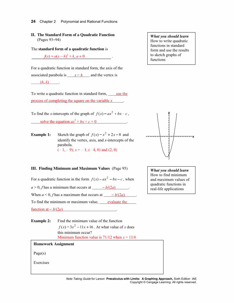
Example 1: Sketch the graph of 82)( 2 xxxf and

identify the vertex, axis, and x-intercepts of the parabola.

( 1, 9); x = 1; ( 4, 0) and (2, 0) III. Finding Minimum and Maximum Values (Page 95) For a quadratic function in the form cbxaxxf 2)( , when

a > 0, f has a minimum that occurs at b/(2a) .

When a < 0, f has a maximum that occurs at b/(2a) .

To find the minimum or maximum value, evaluate the

function at b/(2a) .

Example 2: Find the minimum value of the function

16113)( 2 xxxf . At what value of x does this minimum occur?

Minimum function value is 71/12 when x = 11/6

What you should learn How to write quadratic functions in standard form and use the results to sketch graphs of functions

What you should learn How to find minimum and maximum values of quadratic functions in real-life applications

Homework Assignment Page(s) Exercises

y

x

Section 2.2 Polynomial Functions of Higher Degree 25 Name ___________________________________________________________ Date ____________


Section 2.2 Polynomial Functions of Higher Degree Objective: In this lesson you learned how to sketch and analyze graphs

of polynomial functions. I. Graphs of Polynomial Functions (Pages 100 101) Name two basic features of the graphs of polynomial functions.

1) continuous 2) smooth rounded turns Will the graph of 7)( xxg look more like the graph of

2)( xxf or the graph of 3)( xxf ? Explain. The graph will look more like that of f(x) = x3 because the degree of both is odd. II. The Leading Coefficient Test (Pages 102 103) State the Leading Coefficient Test. As x moves without bound to the left or to the right, the graph of the polynomial function f(x) = anxn + . . . + a1x + a0 eventually rises or falls in the following manner: 1. When n is odd:

a. If the leading coefficient is positive, the graph falls to the left and rises to the right. b. If the leading coefficient is negative, the graph rises to the left and falls to the right.

2. When n is even: a. If the leading coefficient is positive, the graph rises to the left and right. b. If the leading coefficient is negative, the graph falls to the left and right.

Important Vocabulary Define each term or concept. Continuous The graph of a polynomial function has no breaks, holes, or gaps. Extrema The minimums and maximums of a function. Relative minimum The least value of a function on an interval. Relative maximum The greatest value of a function on an interval. Repeated zero If (x – a)k, k > 1, is a factor of a polynomial, then x = a is a repeated zero. Multiplicity The number of times a zero is repeated. Intermediate Value Theorem Let a and b be real numbers such that a < b. If f is a polynomial function such that f(a) f(b), then, in the interval [a, b], f takes on every value between f(a) and f(b).

What you should learn How to use transformations to sketch graphs of polynomial functions

What you should learn How to use the Leading Coefficient Test to determine the end behavior of graphs of polynomial functions



Example 1: Describe the left and right behavior of the graph of 62 431)( xxxf .

Because the degree is even and the leading coefficient is negative, the graph falls to the left and right.

III. Zeros of Polynomial Functions (Pages 104 107) Let f be a polynomial function of degree n. The function f has at

most n real zeros. The graph of f has at most

n 1 relative extrema.

Let f be a polynomial function and let a be a real number. List four equivalent statements about the real zeros of f. 1) x = a is a zero of the function f

2) x = a is a solution of the polynomial equation f(x) = 0

3) (x a) is a factor of the polynomial f(x)

4) (a, 0) is an x-intercept of the graph of f

If a polynomial function f has a repeated zero x = 3 with

multiplicity 4, the graph of f touches the x-axis at

x = 3 . If f has a repeated zero x = 4 with multiplicity 3, the

graph of f crosses the x-axis at x = 4 .

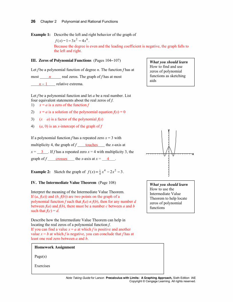
Example 2: Sketch the graph of 32)( 24

41 xxxf .

IV. The Intermediate Value Theorem (Page 108) Interpret the meaning of the Intermediate Value Theorem. If (a, f(a)) and (b, f(b)) are two points on the graph of a polynomial function f such that f(a) f(b), then for any number d between f(a) and f(b), there must be a number c between a and b such that f(c) = d. Describe how the Intermediate Value Theorem can help in locating the real zeros of a polynomial function f. If you can find a value x = a at which f is positive and another value x = b at which f is negative, you can conclude that f has at least one real zero between a and b.

What you should learn How to find and use zeros of polynomial functions as sketching aids


What you should learn How to use the Intermediate Value Theorem to help locate zeros of polynomial functions

y

x

Section 2.3 Real Zeros of Polynomial Functions 27 Name ___________________________________________________________ Date ____________


Section 2.3 Real Zeros of Polynomial Functions Objective: In this lesson you learned how to use long division and

synthetic division to divide polynomials by other polynomials and how to find the rational and real zeros of polynomial functions.

I. Long Division of Polynomials (Pages 113 115) When dividing a polynomial f(x) by another polynomial d(x), if

the remainder r(x) = 0, d(x) divides evenly into f(x).

The rational expression f(x)/d(x) is improper if the degree of

f(x) is greater than or equal to the degree of d(x) .

The rational expression r(x)/d(x) is proper if the degree of

r(x) is less than the degree of d(x) .

Before applying the Division Algorithm, you should write the

dividend and divisor in descending powers of the variable and

insert placeholders with zero coefficients for missing powers of

the variable .

Example 1: Divide 243 3 xx by 122 xx . 3x 6 + (13x + 4)/(x2 + 2x + 1)

Important Vocabulary Define each term or concept. Long division of polynomials A procedure for dividing two polynomials, which is similar to long division in arithmetic. Division Algorithm If f(x) and d(x) are polynomials such that d(x) 0, and the degree of d(x) is less than or equal to the degree of f(x), there exist unique polynomials q(x) and r(x) such that f(x) = d(x)q(x) + r(x) where r(x) = 0 or the degree of r(x) is less than the degree of d(x). Synthetic division A shortcut for long division of polynomials when dividing by divisors of the form x – k. Remainder Theorem If a polynomial f(x) is divided by x – k, then the remainder is r = f(k). Factor Theorem A polynomial f(x) has a factor (x – k) if and only if f(k) = 0. Upper bound A real number b is an upper bound for the real zeros of f if no real zeros of f are greater than b. Lower bound A real number b is a lower bound for the real zeros of f if no real zeros of f are less than b.

What you should learn How to use long division to divide polynomials by other polynomials



II. Synthetic Division (Page 116) Can synthetic division be used to divide a polynomial by x2 5? Explain. No, the divisor must be in the form x k. Can synthetic division be used to divide a polynomial by x + 4? Explain. Yes, rewrite x + 4 as x ( 4). Example 2: Fill in the following synthetic division array to

divide 352 24 xx by x 5. Then carry out the synthetic division and indicate which entry represents the remainder.

5 2 0 5 0 3

10 50 275 1375

2 10 55 275 1372 remainder

III. The Remainder and Factor Theorems (Pages 117 118) To use the Remainder Theorem to evaluate a polynomial

function f(x) at x = k, use synthetic division to divide f(x)

by x k. The remainder will be f(k) .

Example 3: Use the Remainder Theorem to evaluate the

function 352)( 24 xxxf at x = 5. 1372 To use the Factor Theorem to show that (x k) is a factor of a

polynomial function f(x), use synthetic division on f(x)

with the factor (x k). If the remainder is 0, then (x k) is a

factor. Or, alternatively, evaluate f(x) at x = k. If the result is 0,

then (x k) is a factor .

What you should learn How to use synthetic division to divide polynomials by binomials of the form (x k)

What you should learn How to use the Remainder and Factor Theorems

Section 2.3 Real Zeros of Polynomial Functions 29


List three facts about the remainder r, obtained in the synthetic division of f(x) by x k: 1) The remainder r gives the value of f at x = k. That is, r = f(k).

2) If r = 0, (x k) is a factor of f(x).

3) If r = 0, (k, 0) is an x-intercept of the graph of f.

IV. The Rational Zero Test (Pages 119 120) Describe the purpose of the Rational Zero Test.

The Rational Zero Test relates the possible rational zeros of a

polynomial with integer coefficients to the leading coefficient

and to the constant term of the polynomial.

State the Rational Zero Test. If the polynomial f(x) = anxn + an – 1xn – 1 + . . . + a2x2 + a1x + a0

has integer coefficients, every rational zero of f has the form:

rational zero = p/q, where p and q have no common factors other

than 1, p is a factor of the constant term a0, and q is a factor of

the leading coefficient an.

Describe how to use the Rational Zero Test. First list all

rational numbers whose numerators are factors of the constant

term and whose denominators are factors of the leading

coefficient. Then use trial and error to determine which of these

possible rational zeros, if any, are actual zeros of the polynomial.

Example 4: List the possible rational zeros of the polynomial

function 58243)( 2345 xxxxxxf . 1, 5, 1/3, 5/3 List some strategies that can be used to shorten the search for

actual zeros among a list of possible rational zeros.

Using a programmable calculator to speed up the calculations, using

a graphing utility to estimate the locations of zeros, using the

Intermediate Value Theorem (along with a table generated by a

graphing utility) to give approximations of zeros, or using the Factor

Theorem and synthetic division to test possible rational zeros, etc.

What you should learn How to use the Rational Zero Test to determine possible rational zeros of polynomial functions



V. Other Tests for Zeros of Polynomials (Pages 121 123) State the Upper and Lower Bound Rules. Let f(x) be a polynomial with real coefficients and a positive

leading coefficient. Suppose f(x) is divided by x c, using

synthetic division.

1. If c > 0 and each number in the last row is either positive

or zero, c is an upper bound for the real zeros of f.

2. If c < 0 and the numbers in the last row are alternately

positive and negative (zero entries count as positive or

negative), c is a lower bound for the real zeros of f.

Explain how the Upper and Lower Bound Rules can be useful in the search for the real zeros of a polynomial function. Explanations will vary. For instance, suppose you are checking a list of possible rational zeros. When checking the possible rational zero 2 with synthetic division, each number in the last row is positive or zero. Then you need not check any of the other possible rational zeros that are greater than 2 and can concentrate on checking only values less than 2. Additional notes Homework Assignment

Page(s) Exercises

What you should learn How to use Descartes’s Rule of Signs and the Upper and Lower Bound Rules to find zeros of polynomials

y

x

y

x

Section 2.4 Complex Numbers 31 Name ___________________________________________________________ Date ____________


Section 2.4 Complex Numbers Objective: In this lesson you learned how to perform operations with

complex numbers. I. The Imaginary Unit i (Page 128) Mathematicians created an expanded system of numbers using

the imaginary unit i, defined as i = 1 , because

there is no real number x that can be squared to produce 1.

By definition, i2 = 1 .

For the complex number a + bi, if b = 0, the number a + bi = a is

a(n) real number . If b 0, the number a + bi is a(n)

imaginary number . If a = 0, the number a + bi = b,

where 0b , is called a(n) pure imaginary number .

The set of complex numbers consists of the set of real

numbers and the set of imaginary numbers .

Two complex numbers a + bi and c + di, written in standard

form, are equal to each other if and only if a = c and b = d .

II. Operations with Complex Numbers (Pages 129 130) To add two complex numbers, add the real parts and the

imaginary parts of the numbers separately .

To subtract two complex numbers, subtract the real parts and

the imaginary parts of the numbers separately .

The additive identity in the complex number system is 0 . The

additive inverse of the complex number a + bi is (a + bi) = a bi .

Important Vocabulary Define each term or concept. Complex number If a and b are real numbers, the number a + bi, where the number a is called the real part and the number bi is called the imaginary part, is a complex number written in standard form. Complex conjugates A pair of complex numbers of the form a + bi and a – bi.

What you should learn How to use the imaginary unit i to write complex numbers

What you should learn How to add, subtract, and multiply complex numbers


Note Taking Guide for Larson Precalculus with Limits: A Graphing Approach, Sixth Edition IAE Copyright Copyright © Cengage Learning. All rights reserved.

Example 1: Perform the operations: (5 6i) (3 2i) + 4i

2 To multiply two complex numbers a + bi and c + di, use the

multiplication rule (ac bd) + (ad + bc)i or use the Distributive

Property to multiply the two complex numbers, similar to using

the FOIL method for multiplying two binomials .

Example 2: Multiply: (5 6i)(3 2i)

3 28i III. Complex Conjugates (Page 131) The product of a pair of complex conjugates is a(n)

real number.

To find the quotient of the complex numbers a + bi and c + di,

where c and d are not both zero, multiply the numerator and

denominator by the complex conjugate of the denominator .

Example 3: Divide (1 + i) by (2 i). Write the result in

standard form. 1/5 + 3/5i

IV. Complex Solutions of Quadratic Equations (Page 132) When using the Quadratic Formula to solve a quadratic equation,

you may obtain a result such as 7 , which is not a real

number . By factoring out 1i , you can write this

number in standard form .

If a is a positive number, then the principal square root of the

negative number –a is defined as a ai .

What you should learn How to use complex conjugates to write the quotient of two complex numbers in standard form


What you should learn How to find complex solutions of quadratic equations

Section 2.5 The Fundamental Theorem of Algebra 33 Name ___________________________________________________________ Date ____________


Section 2.5 The Fundamental Theorem of Algebra Objective: In this lesson you learned how to determine the numbers of

zeros of polynomial functions and find them. I. The Fundamental Theorem of Algebra (Page 135) In the complex number system, every nth-degree polynomial

function has precisely n zeros.

Example 1: How many zeros does the polynomial function

532 1225)( xxxxf have? 5 An nth-degree polynomial can be factored into

precisely n linear factors.

II. Finding Zeros of a Polynomial Function (Page 136) Remember that the n zeros of a polynomial function can be real

or complex, and they may be repeated .

Example 2: List all of the zeros of the polynomial function

72362)( 23 xxxxf . 2, 6i, 6i III. Conjugate Pairs (Page 137) Let f(x) be a polynomial function that has real coefficients. If

a + bi, where b 0, is a zero of the function, then we know that

a bi is also a zero of the function.

Important Vocabulary Define each term or concept. Fundamental Theorem of Algebra If f(x) is a polynomial of degree n, where n > 0, then f has at least one zero in the complex number system. Linear Factorization Theorem If f(x) is a polynomial of degree n, where n > 0, f has precisely n linear factors f(x) = an(x – c1)( x – c2) . . . (x – cn) where c1, c2, . . . , cn are complex numbers. Conjugates A pair of complex numbers of the form a + bi and a – bi.

What you should learn How to use the Fundamental Theorem of Algebra to determine the number of zeros of a polynomial function

What you should learn How to find conjugate pairs of complex zeros

What you should learn How to find all zeros of polynomial functions, including complex zeros



IV. Factoring a Polynomial (Pages 138 139) To write a polynomial of degree n > 0 with real coefficients as a

product without complex factors, write the polynomial as the

product of linear and/or quadratic factors with real coefficients,

where the quadratic factors have no real zeros .

A quadratic factor with no real zeros is said to be

prime or irreducible over the reals .

Example 3: Write the polynomial 365)( 24 xxxf

(a) as the product of linear factors and quadratic factors that are irreducible over the reals, and

(b) in completely factored form. (a) f(x) = (x + 2)(x 2)(x2 + 9) (b) f(x) = (x + 2)(x 2)(x + 3i)(x 3i) Explain why a graph cannot be used to locate complex zeros. Real zeros are the only zeros that appear as x-intercepts on a graph. A polynomial function’s complex zeros must be found algebraically. Additional notes

What you should learn How to find zeros of polynomials by factoring


y

x

Section 2.6 Rational Functions and Asymptotes 35 Name ___________________________________________________________ Date ____________


Section 2.6 Rational Functions and Asymptotes Objective: In this lesson you learned how to determine the domains and

find asymptotes of rational functions. I. Introduction to Rational Functions (Page 142) The domain of a rational function of x includes all real numbers

except x-values that make the denominator zero .

To find the domain of a rational function of x, set the

denominator of the rational function equal to zero and solve for

x. These values of x must be excluded from the domain of the

function .

Example 1: Find the domain of the function 9

1)(2x

xf .

The domain of f is all real numbers except x = 3 and x = 3.

II. Vertical and Horizontal Asymptotes (Pages 143 145) The notation “f(x) 5 as x ” means that f(x)

approaches 5 as x increases without bound .

Let f be the rational function given by

01

11

011

1

)()()(

bxbxbxbaxaxaxa

xDxNxf

mm

mm

nn

nn

""

where N(x) and D(x) have no common factors. 1) The graph of f has vertical asymptotes at the zeros

of D(x) .

Important Vocabulary Define each term or concept. Rational function A function that can be written in the form: f(x) = N(x)/D(x), where N(x) and D(x) are polynomials and D(x) is not the zero polynomial. Vertical asymptote The line x = a is a vertical asymptote of the graph of f if f(x) or f(x) – as x a , either from the right or from the left. Horizontal asymptote The line y = b is a horizontal asymptote of the graph of f if f(x) b as x or x – .

What you should learn How to find the domains of rational functions

What you should learn How to find vertical and horizontal asymptotes of graphs of rational functions



2) The graph of f has at most one horizontal asymptote

determined by comparing the degrees of N(x) and

D(x) .

a) If n < m, the line y = 0 (the x-axis) is a

horizontal asymptote .

b) If n = m, the line y = an/bm is a horizontal

asymptote .

c) If n > m, the graph of f has no horizontal

asymptote .

Example 2: Find the asymptotes of the function

612)(

2 xxxxf .

Vertical: x = 2, x = 3; Horizontal: y = 0 III. Application of Rational Functions (6) Give an example of asymptotic behavior that occurs in real life. Answers will vary.

What you should learn How to use rational functions to model and solve real-life problems


y

x

y

x

y

x

Section 2.7 Graphs of Rational Functions 37 Name ___________________________________________________________ Date ____________


Section 2.7 Graphs of Rational Functions Objective: In this lesson you learned how to sketch graphs of rational

functions. I. The Graph of a Rational Function (Pages 151 154) List the guidelines for sketching the graph of the rational function

f(x) = N(x)/D(x), where N(x) and D(x) are polynomials.

1) Simplify f, if possible. Any restrictions on the domain of f not

in the simplified function should be listed.

2) Find and plot the y-intercept (if any) by evaluating f(0).

3) Find the zeros of the numerator (if any) by setting the

numerator equal to zero. Then plot the corresponding x-

intercepts.

4) Find the zeros of the denominator (if any) by setting the

denominator equal to zero. Then sketch the corresponding

vertical asymptotes using dashed vertical lines and plot the

corresponding holes using open circles.

5) Find and sketch any other asymptotes of the graph using

dashed lines.

6) Plot at least one point between and one point beyond each

x-intercept and vertical asymptote.

7) Use smooth curves to complete the graph between and

beyond the vertical asymptotes, excluding any points where f is

not defined.

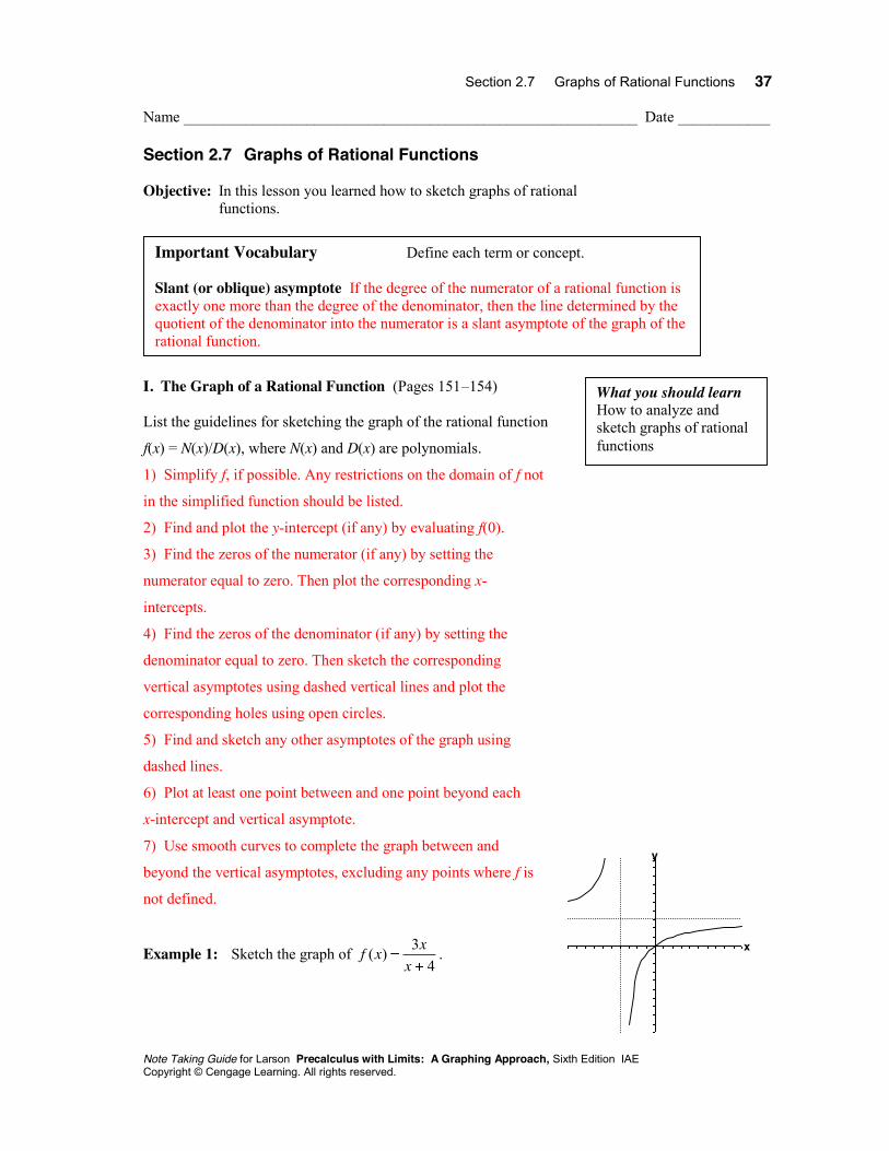
Example 1: Sketch the graph of 4

3)(xxxf .

Important Vocabulary Define each term or concept. Slant (or oblique) asymptote If the degree of the numerator of a rational function is exactly one more than the degree of the denominator, then the line determined by the quotient of the denominator into the numerator is a slant asymptote of the graph of the rational function.

What you should learn How to analyze and sketch graphs of rational functions

y

x



II. Slant Asymptotes (Page 155) Describe how to find the equation of a slant asymptote.

Use long division to divide the denominator of the rational

function into the numerator. The equation of the slant asymptote

is the quotient, excluding the remainder.

Example 2: Decide whether each of the following rational

functions has a slant asymptote. If so, find the equation of the slant asymptote.

(a) 53

1)(2

3

xxxxf (b)

5223)(

3

xxxf

(a) Yes, y = x 3 (b) No III. Applications of Graphs of Rational Functions (Page 156) Describe a real-life situation in which a graph of a rational function would be helpful when solving a problem. Answers will vary.

What you should learn How to sketch graphs of rational functions that have slant asymptotes


y

x

y

x

y

x

What you should learn How to use graphs of rational functions to model and solve real-life problems

Section 2.8 Quadratic Models 39 Name ___________________________________________________________ Date ____________


Section 2.8 Quadratic Models Objective: In this lesson you learned how to classify scatter plots and

use a graphing utility to find quadratic models for data. I. Classifying Scatter Plots (Page 161) Describe how to decide whether a set of data can be modeled by a linear model.

Make a scatter plot of the ordered pairs, either by hand or by

entering the data into a graphing utility and displaying a scatter

plot. Examine the shape of the scatter plot. If it appears that the

data follows a linear pattern, it can be modeled by a linear

function.

Describe how to decide whether a set of data can be modeled by a quadratic model.

Make a scatter plot of the ordered pairs, either by hand or by

entering the data into a graphing utility and displaying a scatter

plot. Examine the shape of the scatter plot. If it appears that the

data follows a parabolic pattern, it can be modeled by a quadratic

function.

II. Fitting a Quadratic Model to Data (Pages 162 163) Once it has been determined that a quadratic model is

appropriate for a set of data, a quadratic model can be fit to data

by entering the data into a graphing utility and using the

regression feature .

Example 1: Find a model that best fits the data given in the

table. y = 0.25x2 5x + 3.45

What you should learn How to classify scatter plots

What you should learn How to use scatter plots and a graphing utility to find quadratic models for data

x 1 0 2 5 9 12 15 y 8.7 3.45 5.55 15.3 21.3 20.55 15.3



III. Choosing a Model (Page 164) If it isn’t easy to tell from a scatter plot which type of model a

set of data would best be modeled by, you should first find

several models for the data and then choose the model that best

fits the data by comparing the y-values of each model with the

actual y-values .

Homework Assignment

Page(s) Exercises

y

x

y

x

y

x

What you should learn How to choose a model that best fits a set of data

y

x

y

x

y

x

chapter 2 polynomial and rational functions for chapter 2.pdf · the leading coefficient test ......

Documents