chapter 2 motion in one dimension - wikispaces this chapter we consider only motion in one...

23

Motion in One Dimension

CHAPTE R OUTL I N E

2.1 Position, Velocity, and Speed

2.2 Instantaneous Velocity andSpeed

2.3 Acceleration

2.4 Motion Diagrams

2.5 One-Dimensional Motion withConstant Acceleration

2.6 Freely Falling Objects

2.7 Kinematic Equations Derivedfrom Calculus

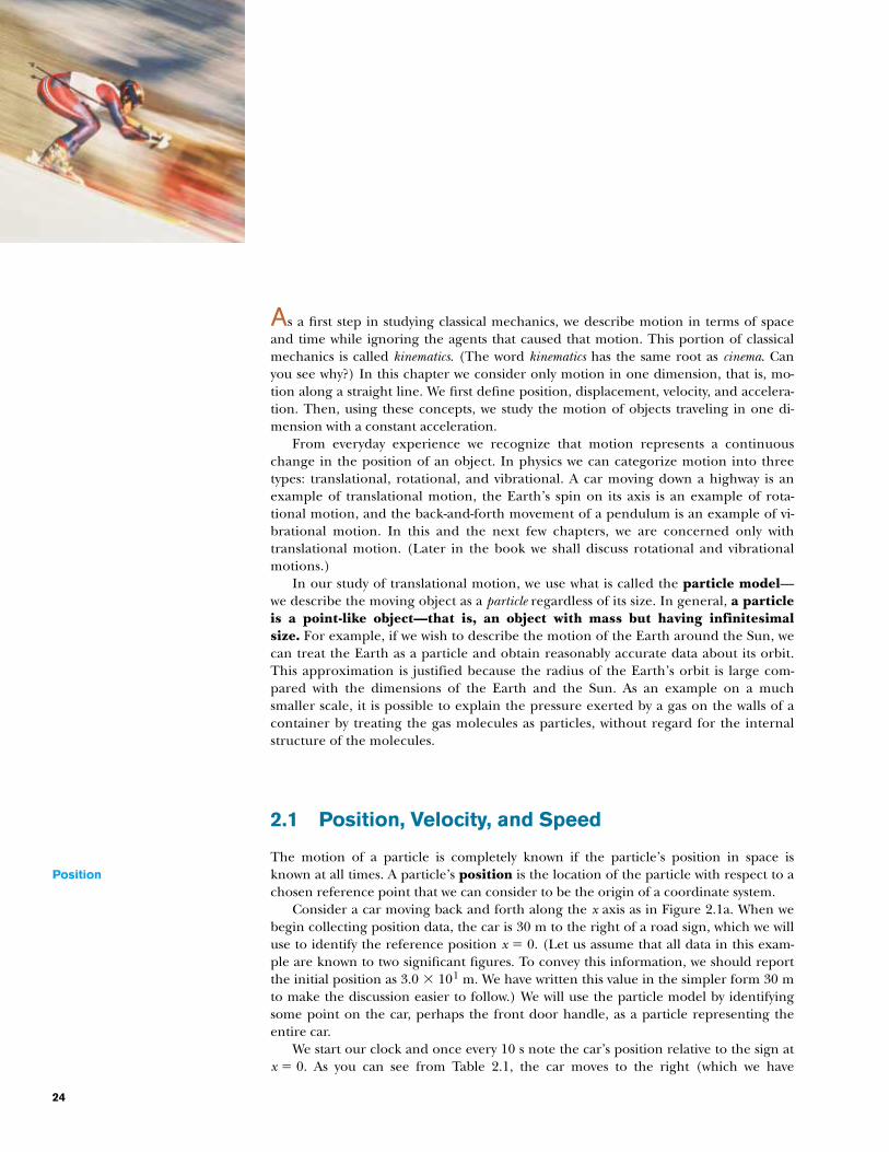
! One of the physical quantities we will study in this chapter is the velocity of an objectmoving in a straight line. Downhill skiers can reach velocities with a magnitude greater than100 km/h. (Jean Y. Ruszniewski/Getty Images)

Chapter 2

General Problem-SolvingStrategy

24

Position

As a first step in studying classical mechanics, we describe motion in terms of spaceand time while ignoring the agents that caused that motion. This portion of classicalmechanics is called kinematics. (The word kinematics has the same root as cinema. Canyou see why?) In this chapter we consider only motion in one dimension, that is, mo-tion along a straight line. We first define position, displacement, velocity, and accelera-tion. Then, using these concepts, we study the motion of objects traveling in one di-mension with a constant acceleration.

From everyday experience we recognize that motion represents a continuouschange in the position of an object. In physics we can categorize motion into threetypes: translational, rotational, and vibrational. A car moving down a highway is anexample of translational motion, the Earth’s spin on its axis is an example of rota-tional motion, and the back-and-forth movement of a pendulum is an example of vi-brational motion. In this and the next few chapters, we are concerned only withtranslational motion. (Later in the book we shall discuss rotational and vibrationalmotions.)

In our study of translational motion, we use what is called the particle model—we describe the moving object as a particle regardless of its size. In general, a particleis a point-like object—that is, an object with mass but having infinitesimalsize. For example, if we wish to describe the motion of the Earth around the Sun, wecan treat the Earth as a particle and obtain reasonably accurate data about its orbit.This approximation is justified because the radius of the Earth’s orbit is large com-pared with the dimensions of the Earth and the Sun. As an example on a muchsmaller scale, it is possible to explain the pressure exerted by a gas on the walls of acontainer by treating the gas molecules as particles, without regard for the internalstructure of the molecules.

2.1 Position, Velocity, and Speed

The motion of a particle is completely known if the particle’s position in space isknown at all times. A particle’s position is the location of the particle with respect to achosen reference point that we can consider to be the origin of a coordinate system.

Consider a car moving back and forth along the x axis as in Figure 2.1a. When webegin collecting position data, the car is 30 m to the right of a road sign, which we willuse to identify the reference position x ! 0. (Let us assume that all data in this exam-ple are known to two significant figures. To convey this information, we should reportthe initial position as 3.0 " 101 m. We have written this value in the simpler form 30 mto make the discussion easier to follow.) We will use the particle model by identifyingsome point on the car, perhaps the front door handle, as a particle representing theentire car.

We start our clock and once every 10 s note the car’s position relative to the sign atx ! 0. As you can see from Table 2.1, the car moves to the right (which we have

S E C T I O N 2 . 1 • Position, Velocity, and Speed 25

!

"

#

$

%

–60–50

–40–30

–20–10

010

2030

4050

60

LIMIT

30 km/h

x(m)

–60–50

–40–30

–20–10

010

2030

4050

60

LIMIT

30 km/h

x(m)

(a)

&

!

10 20 30 40 500

–40

–60

–20

0

20

40

60

∆t

∆x

x(m)

t(s)

(b)

"

#

$

%

&

Active Figure 2.1 (a) A car moves back andforth along a straight line taken to be the xaxis. Because we are interested only in thecar’s translational motion, we can model it asa particle. (b) Position–time graph for themotion of the “particle.”

Position t(s) x(m)

! 0 30" 10 52# 20 38$ 30 0% 40 #37& 50 #53

Table 2.1Position of the Car at Various Times

defined as the positive direction) during the first 10 s of motion, from position ! toposition ". After ", the position values begin to decrease, suggesting that the car isbacking up from position " through position &. In fact, at $, 30 s after we start mea-suring, the car is alongside the road sign (see Figure 2.1a) that we are using to markour origin of coordinates. It continues moving to the left and is more than 50 m to theleft of the sign when we stop recording information after our sixth data point. A graph-ical representation of this information is presented in Figure 2.1b. Such a plot is calleda position–time graph.

Given the data in Table 2.1, we can easily determine the change in position of thecar for various time intervals. The displacement of a particle is defined as its changein position in some time interval. As it moves from an initial position xi to a final posi-tion xf , the displacement of the particle is given by xf # x i . We use the Greek letterdelta ($) to denote the change in a quantity. Therefore, we write the displacement, orchange in position, of the particle as

(2.1)$x ! xf # xi

Displacement

At the Active Figures link athttp://www.pse6.com, you can moveeach of the six points ! through & andobserve the motion of the car pictoriallyand graphically as it follows a smoothpath through the six points.

26 C H A P T E R 2 • Motion in One Dimension

From this definition we see that $x is positive if xf is greater than xi and negative if xf isless than xi.

It is very important to recognize the difference between displacement and distancetraveled. Distance is the length of a path followed by a particle. Consider, for example,the basketball players in Figure 2.2. If a player runs from his own basket down thecourt to the other team’s basket and then returns to his own basket, the displacement ofthe player during this time interval is zero, because he ended up at the same point ashe started. During this time interval, however, he covered a distance of twice the lengthof the basketball court.

Displacement is an example of a vector quantity. Many other physical quantities, in-cluding position, velocity, and acceleration, also are vectors. In general, a vector quan-tity requires the specification of both direction and magnitude. By contrast, ascalar quantity has a numerical value and no direction. In this chapter, we use pos-itive (%) and negative (#) signs to indicate vector direction. We can do this becausethe chapter deals with one-dimensional motion only; this means that any object westudy can be moving only along a straight line. For example, for horizontal motion letus arbitrarily specify to the right as being the positive direction. It follows that any object always moving to the right undergoes a positive displacement $x & 0, and any object moving to the left undergoes a negative displacement, so that $x ' 0. Weshall treat vector quantities in greater detail in Chapter 3.

For our basketball player in Figure 2.2, if the trip from his own basket to the oppos-ing basket is described by a displacement of % 28 m, the trip in the reverse directionrepresents a displacement of # 28 m. Each trip, however, represents a distance of28 m, because distance is a scalar quantity. The total distance for the trip down thecourt and back is 56 m. Distance, therefore, is always represented as a positive number,while displacement can be either positive or negative.

There is one very important point that has not yet been mentioned. Note that thedata in Table 2.1 results only in the six data points in the graph in Figure 2.1b. Thesmooth curve drawn through the six points in the graph is only a possibility of the actualmotion of the car. We only have information about six instants of time—we have noidea what happened in between the data points. The smooth curve is a guess as to whathappened, but keep in mind that it is only a guess.

If the smooth curve does represent the actual motion of the car, the graph con-tains information about the entire 50-s interval during which we watch the car move.It is much easier to see changes in position from the graph than from a verbal de-scription or even a table of numbers. For example, it is clear that the car was cover-ing more ground during the middle of the 50-s interval than at the end. Between po-sitions # and $, the car traveled almost 40 m, but during the last 10 s, betweenpositions % and &, it moved less than half that far. A common way of comparingthese different motions is to divide the displacement $x that occurs between twoclock readings by the length of that particular time interval $t. This turns out to be avery useful ratio, one that we shall use many times. This ratio has been given a specialname—average velocity. The average velocity v–x of a particle is defined as the

Figure 2.2 On this basketball court,players run back and forth for the entiregame. The distance that the players runover the duration of the game is non-zero. The displacement of the playersover the duration of the game isapproximately zero because they keepreturning to the same point over andover again.Ke

n W

hite

/Alls

port/

Getty

Imag

es

Average speed

S E C T I O N 2 . 1 • Position, Velocity, and Speed 27

particle’s displacement ∆x divided by the time interval ∆t during which thatdisplacement occurs:

(2.2)

where the subscript x indicates motion along the x axis. From this definition we seethat average velocity has dimensions of length divided by time (L/T)—meters per sec-ond in SI units.

The average velocity of a particle moving in one dimension can be positive or nega-tive, depending on the sign of the displacement. (The time interval $t is always posi-tive.) If the coordinate of the particle increases in time (that is, if xf & x i ), then $x ispositive and is positive. This case corresponds to a particle moving in thepositive x direction, that is, toward larger values of x. If the coordinate decreases intime (that is, if xf ' x i ) then $x is negative and hence is negative. This case corre-sponds to a particle moving in the negative x direction.

We can interpret average velocity geometrically by drawing a straight line betweenany two points on the position–time graph in Figure 2.1b. This line forms the hy-potenuse of a right triangle of height $x and base $t. The slope of this line is the ratio$x/$t, which is what we have defined as average velocity in Equation 2.2. For example,the line between positions ! and " in Figure 2.1b has a slope equal to the average ve-locity of the car between those two times, (52 m # 30 m)/(10 s # 0) ! 2.2 m/s.

In everyday usage, the terms speed and velocity are interchangeable. In physics, how-ever, there is a clear distinction between these two quantities. Consider a marathonrunner who runs more than 40 km, yet ends up at his starting point. His total displace-ment is zero, so his average velocity is zero! Nonetheless, we need to be able to quantifyhow fast he was running. A slightly different ratio accomplishes this for us. The aver-age speed of a particle, a scalar quantity, is defined as the total distance traveled di-vided by the total time interval required to travel that distance:

(2.3)

The SI unit of average speed is the same as the unit of average velocity: meters per sec-ond. However, unlike average velocity, average speed has no direction and hence car-ries no algebraic sign. Notice the distinction between average velocity and averagespeed—average velocity (Eq. 2.2) is the displacement divided by the time interval, whileaverage speed (Eq. 2.3) is the distance divided by the time interval.

Knowledge of the average velocity or average speed of a particle does not provide in-formation about the details of the trip. For example, suppose it takes you 45.0 s to travel100 m down a long straight hallway toward your departure gate at an airport. At the 100-mmark, you realize you missed the rest room, and you return back 25.0 m along the same hallway, taking 10.0 s to make the return trip. The magnitude of the average velocity for your trip is % 75.0 m/55.0 s ! % 1.36 m/s. The average speed for your trip is125 m/55.0 s ! 2.27 m/s. You may have traveled at various speeds during the walk. Nei-ther average velocity nor average speed provides information about these details.

Average speed !total distance

total time

vx

vx ! $x/$t

vx ! $x$t

! PITFALL PREVENTION2.1 Average Speed and

Average VelocityThe magnitude of the average ve-locity is not the average speed.For example, consider themarathon runner discussed here.The magnitude of the average ve-locity is zero, but the averagespeed is clearly not zero.

Quick Quiz 2.1 Under which of the following conditions is the magnitude ofthe average velocity of a particle moving in one dimension smaller than the averagespeed over some time interval? (a) A particle moves in the % x direction without revers-ing. (b) A particle moves in the # x direction without reversing. (c) A particle moves inthe % x direction and then reverses the direction of its motion. (d) There are no con-ditions for which this is true.

Average velocity

Example 2.1 Calculating the Average Velocity and Speed


2.2 Instantaneous Velocity and Speed

Often we need to know the velocity of a particle at a particular instant in time, ratherthan the average velocity over a finite time interval. For example, even though youmight want to calculate your average velocity during a long automobile trip, you wouldbe especially interested in knowing your velocity at the instant you noticed the policecar parked alongside the road ahead of you. In other words, you would like to be ableto specify your velocity just as precisely as you can specify your position by noting whatis happening at a specific clock reading—that is, at some specific instant. It may not beimmediately obvious how to do this. What does it mean to talk about how fast some-thing is moving if we “freeze time” and talk only about an individual instant? This is asubtle point not thoroughly understood until the late 1600s. At that time, with the in-vention of calculus, scientists began to understand how to describe an object’s motionat any moment in time.

To see how this is done, consider Figure 2.3a, which is a reproduction of the graphin Figure 2.1b. We have already discussed the average velocity for the interval duringwhich the car moved from position ! to position " (given by the slope of the darkblue line) and for the interval during which it moved from ! to & (represented bythe slope of the light blue line and calculated in Example 2.1). Which of these twolines do you think is a closer approximation of the initial velocity of the car? The carstarts out by moving to the right, which we defined to be the positive direction. There-fore, being positive, the value of the average velocity during the ! to " interval ismore representative of the initial value than is the value of the average velocity duringthe ! to & interval, which we determined to be negative in Example 2.1. Now let usfocus on the dark blue line and slide point " to the left along the curve, toward point!, as in Figure 2.3b. The line between the points becomes steeper and steeper, and asthe two points become extremely close together, the line becomes a tangent line tothe curve, indicated by the green line in Figure 2.3b. The slope of this tangent line

! PITFALL PREVENTION2.2 Slopes of GraphsIn any graph of physical data, theslope represents the ratio of thechange in the quantity repre-sented on the vertical axis to thechange in the quantity repre-sented on the horizontal axis. Re-member that a slope has units (un-less both axes have the sameunits). The units of slope inFigure 2.1b and Figure 2.3 arem/s, the units of velocity.

Find the displacement, average velocity, and average speedof the car in Figure 2.1a between positions ! and &.

Solution From the position–time graph given in Figure2.1b, note that xA ! 30 m at tA ! 0 s and that x F ! # 53 mat t F ! 50 s. Using these values along with the definition ofdisplacement, Equation 2.1, we find that

This result means that the car ends up 83 m in the nega-tive direction (to the left, in this case) from where itstarted. This number has the correct units and is of thesame order of magnitude as the supplied data. Aquick look at Figure 2.1a indicates that this is the correctanswer.

It is difficult to estimate the average velocity withoutcompleting the calculation, but we expect the units to bemeters per second. Because the car ends up to the left ofwhere we started taking data, we know the average velocitymust be negative. From Equation 2.2,

#83 m$x ! x F # xA ! #53 m # 30 m ! We cannot unambiguously find the average speed of thecar from the data in Table 2.1, because we do not have infor-mation about the positions of the car between the datapoints. If we adopt the assumption that the details of thecar’s position are described by the curve in Figure 2.1b, thenthe distance traveled is 22 m (from ! to ") plus 105 m(from " to &) for a total of 127 m. We find the car’s averagespeed for this trip by dividing the distance by the total time(Eq. 2.3):

2.5 m/sAverage speed !127 m50 s

!

#1.7 m/s!

!#53 m # 30 m

50 s # 0 s!

#83 m50 s

vx !$x$t

!xf # xi

tf # ti!

xF # xA

tF # tA

S E C T I O N 2 . 2 • Instantaneous Velocity and Speed 29

x(m)

t(s)

(a)50403020100

60

20

0

–20

–40

–60

!

$

%

&

#

"

40

60

40

(b)

"

!

"""

represents the velocity of the car at the moment we started taking data, at point !.What we have done is determine the instantaneous velocity at that moment. In otherwords, the instantaneous velocity vx equals the limiting value of the ratio !x(!tas !t approaches zero:1

(2.4)

In calculus notation, this limit is called the derivative of x with respect to t, written dx/dt:

(2.5)

The instantaneous velocity can be positive, negative, or zero. When the slope of theposition–time graph is positive, such as at any time during the first 10 s in Figure 2.3,vx is positive—the car is moving toward larger values of x. After point ", vx is nega-tive because the slope is negative—the car is moving toward smaller values of x. Atpoint ", the slope and the instantaneous velocity are zero—the car is momentarily atrest.

From here on, we use the word velocity to designate instantaneous velocity. When itis average velocity we are interested in, we shall always use the adjective average.

The instantaneous speed of a particle is defined as the magnitude of its instan-taneous velocity. As with average speed, instantaneous speed has no directionassociated with it and hence carries no algebraic sign. For example, if one particlehas an instantaneous velocity of % 25 m/s along a given line and another particlehas an instantaneous velocity of # 25 m/s along the same line, both have a speed2

of 25 m/s.

vx ! lim$t : 0

$x$t

!dxdt

vx ! lim$t : 0

$x$t

Active Figure 2.3 (a) Graph representing the motion of the car in Figure 2.1. (b) Anenlargement of the upper-left-hand corner of the graph shows how the blue linebetween positions ! and " approaches the green tangent line as point " is movedcloser to point !.

At the Active Figures link at http://www.pse6.com, you can move point "as suggested in (b) and observe the blue line approaching the green tangentline.

Instantaneous velocity

1 Note that the displacement $x also approaches zero as $t approaches zero, so that the ratiolooks like 0/0. As $x and $t become smaller and smaller, the ratio $x/$t approaches a valueequal to the slope of the line tangent to the x-versus-t curve.2 As with velocity, we drop the adjective for instantaneous speed: “Speed” means instantaneousspeed.

! PITFALL PREVENTION2.3 Instantaneous Speed

and InstantaneousVelocity

In Pitfall Prevention 2.1, we ar-gued that the magnitude of theaverage velocity is not the averagespeed. Notice the differencewhen discussing instantaneousvalues. The magnitude of the in-stantaneous velocity is the instan-taneous speed. In an infinitesimaltime interval, the magnitude ofthe displacement is equal to thedistance traveled by the particle.

A particle moves along the x axis. Its position varies withtime according to the expression x ! # 4t % 2t 2 where x isin meters and t is in seconds.3 The position–time graph forthis motion is shown in Figure 2.4. Note that the particlemoves in the negative x direction for the first second of mo-tion, is momentarily at rest at the moment t ! 1 s, andmoves in the positive x direction at times t & 1 s.

(A) Determine the displacement of the particle in the timeintervals t ! 0 to t ! 1 s and t ! 1 s to t ! 3 s.

Solution During the first time interval, the slope is nega-tive and hence the average velocity is negative. Thus, weknow that the displacement between ! and " must be anegative number having units of meters. Similarly, we expectthe displacement between " and $ to be positive.

In the first time interval, we set ti ! tA ! 0 andtf ! t B ! 1 s. Using Equation 2.1, with x ! # 4t % 2t 2, weobtain for the displacement between t ! 0 and t ! 1 s,

To calculate the displacement during the second time inter-val (t ! 1 s to t ! 3 s), we set ti ! tB ! 1 s and tf ! tD ! 3 s:

These displacements can also be read directly from the posi-tion–time graph.

(B) Calculate the average velocity during these two time in-tervals.

Solution In the first time interval, $t ! tf # ti !t B # tA ! 1 s. Therefore, using Equation 2.2 and the dis-placement calculated in (a), we find that

#2 m/svx(A : B) !$xA : B

$t!

#2 m1 s

!

%8 m!

! [#4(3) % 2(3)2] # [#4(1) % 2(1)2]

$x B : D ! xf # xi ! x D # x B

#2 m !

! [#4(1) % 2(1)2] # [#4(0) % 2(0)2]

$xA : B ! xf # xi ! xB # xA


Conceptual Example 2.2 The Velocity of Different Objects

Example 2.3 Average and Instantaneous Velocity

Consider the following one-dimensional motions: (A) A ballthrown directly upward rises to a highest point and fallsback into the thrower’s hand. (B) A race car starts from restand speeds up to 100 m/s. (C) A spacecraft drifts throughspace at constant velocity. Are there any points in the mo-tion of these objects at which the instantaneous velocity hasthe same value as the average velocity over the entire mo-tion? If so, identify the point(s).

Solution (A) The average velocity for the thrown ball iszero because the ball returns to the starting point; thus itsdisplacement is zero. (Remember that average velocity isdefined as $x/$t.) There is one point at which the instanta-neous velocity is zero—at the top of the motion.

(B) The car’s average velocity cannot be evaluated unam-biguously with the information given, but it must be somevalue between 0 and 100 m/s. Because the car will haveevery instantaneous velocity between 0 and 100 m/s atsome time during the interval, there must be some instantat which the instantaneous velocity is equal to the averagevelocity.

(C) Because the spacecraft’s instantaneous velocity is con-stant, its instantaneous velocity at any time and its averagevelocity over any time interval are the same.

10

8

6

4

2

0

–2

–40 1 2 3 4

t(s)

x(m)

$

!

"

#

Slope = 4 m/s

Slope = –2 m/s

Figure 2.4 (Example 2.3) Position–time graph for a particlehaving an x coordinate that varies in time according to theexpression x ! # 4t % 2t2.

In the second time interval, $t ! 2 s; therefore,

These values are the same as the slopes of the lines joiningthese points in Figure 2.4.

(C) Find the instantaneous velocity of the particle at t ! 2.5 s.

Solution We can guess that this instantaneous velocity mustbe of the same order of magnitude as our previous results,that is, a few meters per second. By measuring the slope ofthe green line at t ! 2.5 s in Figure 2.4, we find that

%6 m/svx !

%4 m/svx(B : D) !$x B : D

$t!

8 m2 s

!

3 Simply to make it easier to read, we write the expression asx ! #4t % 2t2 rather than as x ! (# 4.00 m/s)t % (2.00 m/s2)t2.00.When an equation summarizes measurements, consider its coeffi-cients to have as many significant digits as other data quoted in aproblem. Consider its coefficients to have the units required for di-mensional consistency. When we start our clocks at t ! 0, we usuallydo not mean to limit the precision to a single digit. Consider anyzero value in this book to have as many significant figures as youneed.

!

"

!

t ft i

vxi

vxf

vx ax =

∆t

∆vx

∆vx∆t

t

(b)

ti tf

(a)

x

v = vxi v = vxf

"

–

S E C T I O N 2 . 3 • Acceleration 31

Figure 2.5 (a) A car, modeled as a particle, moving along the xaxis from ! to " has velocity vxi at t ! ti and velocity vxf at t ! tf.(b) Velocity–time graph (rust) for the particle moving in astraight line. The slope of the blue straight line connecting !and " is the average acceleration in the time interval$t ! tf # ti.

The average acceleration a–x of the particle is defined as the change in velocity$vx divided by the time interval $t during which that change occurs:

2.3 Acceleration

In the last example, we worked with a situation in which the velocity of a particlechanges while the particle is moving. This is an extremely common occurrence. (Howconstant is your velocity as you ride a city bus or drive on city streets?) It is possible toquantify changes in velocity as a function of time similarly to the way in which we quan-tify changes in position as a function of time. When the velocity of a particle changeswith time, the particle is said to be accelerating. For example, the magnitude of thevelocity of a car increases when you step on the gas and decreases when you apply thebrakes. Let us see how to quantify acceleration.

Suppose an object that can be modeled as a particle moving along the x axis has aninitial velocity vxi at time ti and a final velocity vxf at time tf, as in Figure 2.5a.

Average acceleration(2.6)

As with velocity, when the motion being analyzed is one-dimensional, we can usepositive and negative signs to indicate the direction of the acceleration. Because the di-mensions of velocity are L/T and the dimension of time is T, acceleration has dimen-sions of length divided by time squared, or L/T2. The SI unit of acceleration is metersper second squared (m/s2). It might be easier to interpret these units if you think ofthem as meters per second per second. For example, suppose an object has an acceler-ation of % 2 m/s2. You should form a mental image of the object having a velocity thatis along a straight line and is increasing by 2 m/s during every interval of 1 s. If the ob-ject starts from rest, you should be able to picture it moving at a velocity of % 2 m/s af-ter 1 s, at % 4 m/s after 2 s, and so on.

In some situations, the value of the average acceleration may be different overdifferent time intervals. It is therefore useful to define the instantaneous accelerationas the limit of the average acceleration as $t approaches zero. This concept is analo-gous to the definition of instantaneous velocity discussed in the previous section. Ifwe imagine that point ! is brought closer and closer to point " in Figure 2.5a andwe take the limit of $vx/$t as $t approaches zero, we obtain the instantaneousacceleration:

(2.7)ax ! lim$t : 0

$vx

$t!

dvx

dt

ax !

$vx

$t!

vxf # vxi

tf # ti

Instantaneous acceleration

That is, the instantaneous acceleration equals the derivative of the velocitywith respect to time, which by definition is the slope of the velocity–time graph.The slope of the green line in Figure 2.5b is equal to the instantaneous accelerationat point ". Thus, we see that just as the velocity of a moving particle is the slope at apoint on the particle’s x -t graph, the acceleration of a particle is the slope at a pointon the particle’s vx -t graph. One can interpret the derivative of the velocity with re-spect to time as the time rate of change of velocity. If ax is positive, the accelerationis in the positive x direction; if ax is negative, the acceleration is in the negative xdirection.

For the case of motion in a straight line, the direction of the velocity of an objectand the direction of its acceleration are related as follows. When the object’s velocityand acceleration are in the same direction, the object is speeding up. On theother hand, when the object’s velocity and acceleration are in opposite direc-tions, the object is slowing down.

To help with this discussion of the signs of velocity and acceleration, we can relatethe acceleration of an object to the force exerted on the object. In Chapter 5 we for-mally establish that force is proportional to acceleration:

This proportionality indicates that acceleration is caused by force. Furthermore, forceand acceleration are both vectors and the vectors act in the same direction. Thus, letus think about the signs of velocity and acceleration by imagining a force applied to anobject and causing it to accelerate. Let us assume that the velocity and acceleration arein the same direction. This situation corresponds to an object moving in some direc-tion that experiences a force acting in the same direction. In this case, the objectspeeds up! Now suppose the velocity and acceleration are in opposite directions. Inthis situation, the object moves in some direction and experiences a force acting in theopposite direction. Thus, the object slows down! It is very useful to equate the direc-tion of the acceleration to the direction of a force, because it is easier from our every-day experience to think about what effect a force will have on an object than to thinkonly in terms of the direction of the acceleration.

F ) a


Quick Quiz 2.2 If a car is traveling eastward and slowing down, what is thedirection of the force on the car that causes it to slow down? (a) eastward (b) westward(c) neither of these.

t

(b)

ax

tA tB

tC

tA tB tC

(a)

vx

t

Figure 2.6 The instantaneousacceleration can be obtained fromthe velocity–time graph (a). Ateach instant, the acceleration inthe ax versus t graph (b) equals theslope of the line tangent to the vxversus t curve (a).

! PITFALL PREVENTION2.4 Negative

AccelerationKeep in mind that negative acceler-ation does not necessarily mean thatan object is slowing down. If the ac-celeration is negative, and the ve-locity is negative, the object isspeeding up!

! PITFALL PREVENTION2.5 DecelerationThe word deceleration has the com-mon popular connotation of slow-ing down. We will not use this wordin this text, because it further con-fuses the definition we have givenfor negative acceleration.

From now on we shall use the term acceleration to mean instantaneous acceleration.When we mean average acceleration, we shall always use the adjective average.

Because vx ! dx/dt, the acceleration can also be written

(2.8)

That is, in one-dimensional motion, the acceleration equals the second derivative of xwith respect to time.

Figure 2.6 illustrates how an acceleration–time graph is related to a velocity–timegraph. The acceleration at any time is the slope of the velocity–time graph at that time.Positive values of acceleration correspond to those points in Figure 2.6a where the ve-locity is increasing in the positive x direction. The acceleration reaches a maximum attime tA, when the slope of the velocity–time graph is a maximum. The accelerationthen goes to zero at time t B, when the velocity is a maximum (that is, when the slope ofthe vx -t graph is zero). The acceleration is negative when the velocity is decreasing inthe positive x direction, and it reaches its most negative value at time tC.

ax !dvx

dt!

ddt

" dxdt # !

d 2xdt 2

S E C T I O N 2 . 3 • Acceleration 33

Conceptual Example 2.4 Graphical Relationships between x, vx , and ax

(a)

(b)

(c)

x

t Ft Et Dt Ct Bt A

t Ft Et Dt Ct B

tt AO

tO

tO t Ft Et Bt A

v x

a x

Figure 2.7 (Example 2.4) (a) Position–time graph for an ob-ject moving along the x axis. (b) The velocity–time graph forthe object is obtained by measuring the slope of theposition–time graph at each instant. (c) The acceleration–timegraph for the object is obtained by measuring the slope of thevelocity–time graph at each instant.

The position of an object moving along the x axis varies withtime as in Figure 2.7a. Graph the velocity versus time andthe acceleration versus time for the object.

Solution The velocity at any instant is the slope of thetangent to the x -t graph at that instant. Between t ! 0 andt ! tA, the slope of the x -t graph increases uniformly, andso the velocity increases linearly, as shown in Figure 2.7b.Between tA and tB, the slope of the x -t graph is constant,and so the velocity remains constant. At tD, the slope ofthe x -t graph is zero, so the velocity is zero at that instant.Between tD and tE, the slope of the x -t graph and thus thevelocity are negative and decrease uniformly in this inter-val. In the interval tE to tF, the slope of the x-t graph is stillnegative, and at tF it goes to zero. Finally, after tF, theslope of the x -t graph is zero, meaning that the object is atrest for t & tF .

The acceleration at any instant is the slope of the tan-gent to the vx -t graph at that instant. The graph of accelera-tion versus time for this object is shown in Figure 2.7c. Theacceleration is constant and positive between 0 and tA,where the slope of the vx -t graph is positive. It is zero be-tween tA and tB and for t & tF because the slope of the vx -tgraph is zero at these times. It is negative between tB and tEbecause the slope of the vx -t graph is negative during this interval.

Note that the sudden changes in acceleration shown inFigure 2.7c are unphysical. Such instantaneous changes can-not occur in reality.

Quick Quiz 2.3 Make a velocity–time graph for the car in Figure 2.1a. Thespeed limit posted on the road sign is 30 km/h. True or false? The car exceeds thespeed limit at some time within the interval.

Therefore, the average acceleration in the specified time in-terval $t ! t B # t A ! 2.0 s is

The negative sign is consistent with our expectations—namely, that the average acceleration, which is representedby the slope of the line joining the initial and final pointson the velocity–time graph, is negative.

(B) Determine the acceleration at t ! 2.0 s.

#10 m/s2!

ax !vxf # vxi

tf # ti!

vx B # vx A

t B # tA!

(20 # 40) m/s(2.0 # 0) s

vx B ! (40 # 5t B2) m/s ! [40 # 5(2.0)2] m/s ! % 20 m/sThe velocity of a particle moving along the x axis varies in

time according to the expression vx ! (40 # 5t 2 ) m/s,where t is in seconds.

(A) Find the average acceleration in the time interval t ! 0to t ! 2.0 s.

Solution Figure 2.8 is a vx -t graph that was created fromthe velocity versus time expression given in the problemstatement. Because the slope of the entire vx-t curve is nega-tive, we expect the acceleration to be negative.

We find the velocities at ti ! tA ! 0 and tf ! tB ! 2.0 sby substituting these values of t into the expression for thevelocity:

vx A ! (40 # 5tA2) m/s ! [40 # 5(0)2] m/s ! % 40 m/s

Example 2.5 Average and Instantaneous Acceleration

So far we have evaluated the derivatives of a function by starting with the definitionof the function and then taking the limit of a specific ratio. If you are familiar with cal-culus, you should recognize that there are specific rules for taking derivatives. Theserules, which are listed in Appendix B.6, enable us to evaluate derivatives quickly. Forinstance, one rule tells us that the derivative of any constant is zero. As another exam-ple, suppose x is proportional to some power of t, such as in the expression

x ! Atn

where A and n are constants. (This is a very common functional form.) The derivativeof x with respect to t is

Applying this rule to Example 2.5, in which vx ! 40 # 5t 2 , we find that the accelera-tion is ax ! dvx/dt ! #10t .

2.4 Motion Diagrams

The concepts of velocity and acceleration are often confused with each other, but infact they are quite different quantities. It is instructive to use motion diagrams to de-scribe the velocity and acceleration while an object is in motion.

A stroboscopic photograph of a moving object shows several images of the object,taken as the strobe light flashes at a constant rate. Figure 2.9 represents three sets ofstrobe photographs of cars moving along a straight roadway in a single direction, fromleft to right. The time intervals between flashes of the stroboscope are equal in eachpart of the diagram. In order not to confuse the two vector quantities, we use red forvelocity vectors and violet for acceleration vectors in Figure 2.9. The vectors are

dxdt

! nAtn#1


10

–10

0

0 1 2 3 4

t(s)

vx(m/s)

20

30

40

–20

–30

Slope = –20 m/s2

!

"

Figure 2.8 (Example 2.5) The velocity–time graph for aparticle moving along the x axis according to the expressionvx ! (40 # 5t 2) m/s. The acceleration at t ! 2 s is equal to theslope of the green tangent line at that time.

Solution The velocity at any time t is vxi ! (40 # 5t 2 ) m/sand the velocity at any later time t % $t is

Therefore, the change in velocity over the time interval $t is

Dividing this expression by $t and taking the limit of the re-sult as $t approaches zero gives the acceleration at any time t :

Therefore, at t ! 2.0 s,

Because the velocity of the particle is positive and the accel-eration is negative, the particle is slowing down.

Note that the answers to parts (A) and (B) are different.The average acceleration in (A) is the slope of the blue linein Figure 2.8 connecting points ! and ". The instanta-neous acceleration in (B) is the slope of the green linetangent to the curve at point ". Note also that the accelera-tion is not constant in this example. Situations involving con-stant acceleration are treated in Section 2.5.

#20 m/s2ax ! (#10)(2.0) m/s2 !

ax ! lim$t : 0

$vx

$t! lim

$t : 0(#10t # 5$t) ! #10t m/s2

$vx ! vxf # vxi ! [#10t $t # 5($t)2] m/s

vxf ! 40 # 5(t % $t)2 ! 40 # 5t 2 # 10t $t # 5($t)2

sketched at several instants during the motion of the object. Let us describe the mo-tion of the car in each diagram.

In Figure 2.9a, the images of the car are equally spaced, showing us that the carmoves through the same displacement in each time interval. This is consistent with thecar moving with constant positive velocity and zero acceleration. We could model the car as aparticle and describe it as a particle moving with constant velocity.

In Figure 2.9b, the images become farther apart as time progresses. In this case, thevelocity vector increases in time because the car’s displacement between adjacent posi-tions increases in time. This suggests that the car is moving with a positive velocity and apositive acceleration. The velocity and acceleration are in the same direction. In terms ofour earlier force discussion, imagine a force pulling on the car in the same direction itis moving—it speeds up.

In Figure 2.9c, we can tell that the car slows as it moves to the right because its dis-placement between adjacent images decreases with time. In this case, this suggests thatthe car moves to the right with a constant negative acceleration. The velocity vector de-creases in time and eventually reaches zero. From this diagram we see that the acceler-ation and velocity vectors are not in the same direction. The car is moving with a posi-tive velocity but with a negative acceleration. (This type of motion is exhibited by a car thatskids to a stop after applying its brakes.) The velocity and acceleration are in oppositedirections. In terms of our earlier force discussion, imagine a force pulling on the caropposite to the direction it is moving—it slows down.

The violet acceleration vectors in Figures 2.9b and 2.9c are all of the same length.Thus, these diagrams represent motion with constant acceleration. This is an impor-tant type of motion that will be discussed in the next section.

S E C T I O N 2 . 4 • Motion Diagrams 35

(a)

(b)

(c)

v

v

a

v

a

Active Figure 2.9 (a) Motion diagram for a car moving at constant velocity (zeroacceleration). (b) Motion diagram for a car whose constant acceleration is in thedirection of its velocity. The velocity vector at each instant is indicated by a red arrow,and the constant acceleration by a violet arrow. (c) Motion diagram for a car whoseconstant acceleration is in the direction opposite the velocity at each instant.

Quick Quiz 2.4 Which of the following is true? (a) If a car is traveling east-ward, its acceleration is eastward. (b) If a car is slowing down, its acceleration must benegative. (c) A particle with constant acceleration can never stop and stay stopped.

At the Active Figures linkat http://www.pse6.com, youcan select the constantacceleration and initial velocityof the car and observe pictorialand graphical representationsof its motion.

2.5 One-Dimensional Motion with Constant Acceleration

If the acceleration of a particle varies in time, its motion can be complex and difficult toanalyze. However, a very common and simple type of one-dimensional motion is that inwhich the acceleration is constant. When this is the case, the average acceleration overany time interval is numerically equal to the instantaneous acceleration ax at any instantwithin the interval, and the velocity changes at the same rate throughout the motion.

If we replace by ax in Equation 2.6 and take ti ! 0 and tf to be any later time t, wefind that

or

(2.9)

This powerful expression enables us to determine an object’s velocity at any time t if weknow the object’s initial velocity vxi and its (constant) acceleration ax. A velocity–timegraph for this constant-acceleration motion is shown in Figure 2.10b. The graph is astraight line, the (constant) slope of which is the acceleration ax; this is consistent withthe fact that ax ! dvx/dt is a constant. Note that the slope is positive; this indicates apositive acceleration. If the acceleration were negative, then the slope of the line inFigure 2.10b would be negative.

When the acceleration is constant, the graph of acceleration versus time (Fig.2.10c) is a straight line having a slope of zero.

Because velocity at constant acceleration varies linearly in time according to Equa-tion 2.9, we can express the average velocity in any time interval as the arithmeticmean of the initial velocity vxi and the final velocity vxf :

(2.10)

Note that this expression for average velocity applies only in situations in which theacceleration is constant.

We can now use Equations 2.1, 2.2, and 2.10 to obtain the position of an object as afunction of time. Recalling that $x in Equation 2.2 represents xf # xi, and recognizingthat $t ! tf # ti ! t # 0 ! t, we find

(2.11)

This equation provides the final position of the particle at time t in terms of the initialand final velocities.

We can obtain another useful expression for the position of a particle moving withconstant acceleration by substituting Equation 2.9 into Equation 2.11:

(2.12)

This equation provides the final position of the particle at time t in terms of the initialvelocity and the acceleration.

The position–time graph for motion at constant (positive) acceleration shownin Figure 2.10a is obtained from Equation 2.12. Note that the curve is a parabola.

xf ! xi % vxi t % 12 axt 2 (for constant ax)

xf ! xi % 12 [vxi % (vxi % axt)]t

x f ! xi % 12 (vxi % vxf)t (for constant ax)

xf # xi ! vt ! 12 (vxi % vxf)t

vx !vxi % vxf

2 (for constant ax)

vxf ! vxi % axt (for constant ax)

ax !vxf # vxi

t # 0

ax

ax

(b)

vx

vxi

0

vxf

tvxi

axt

t

Slope = ax

(a)

x

0 t

xi

Slope = vxi

t

(c)

ax

0

ax

t

Slope = 0

Slope = vxf

Active Figure 2.10 A particlemoving along the x axis with con-stant acceleration ax; (a) the posi-tion–time graph, (b) thevelocity–time graph, and (c) theacceleration–time graph.


Position as a function ofvelocity and time

Position as a function of time

At the Active Figures linkat http://www.pse6.com, youcan adjust the constantacceleration and observe theeffect on the position andvelocity graphs.

The slope of the tangent line to this curve at t ! 0 equals the initial velocity vxi ,and the slope of the tangent line at any later time t equals the velocity vxf at thattime.

Finally, we can obtain an expression for the final velocity that does not containtime as a variable by substituting the value of t from Equation 2.9 into Equation2.11:

(2.13)

This equation provides the final velocity in terms of the acceleration and the displace-ment of the particle.

For motion at zero acceleration, we see from Equations 2.9 and 2.12 that

vxf ! vxi ! vxwhen ax ! 0

xf ! xi % vxt

That is, when the acceleration of a particle is zero, its velocity is constant and its posi-tion changes linearly with time.

v 2xf ! v 2

xi % 2ax (xf # xi) (for constant ax)

xf ! xi % 12 (vxi % vxf) " vxf # vxi

ax# !

v 2xf # v 2

xi

2a x

t

vx

(a)

t

ax

(d)

t

vx

(b)t

ax

(e)

t

vx

(c)

t

ax

(f)

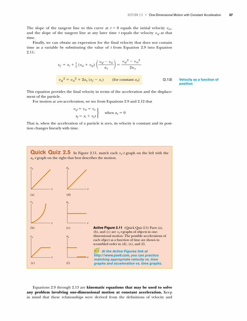
Active Figure 2.11 (Quick Quiz 2.5) Parts (a),(b), and (c) are vx -t graphs of objects in one-dimensional motion. The possible accelerations ofeach object as a function of time are shown inscrambled order in (d), (e), and (f).

Quick Quiz 2.5 In Figure 2.11, match each vx -t graph on the left with theax -t graph on the right that best describes the motion.

S E C T I O N 2 . 5 • One-Dimensional Motion with Constant Acceleration 37

Velocity as a function ofposition

}

Equations 2.9 through 2.13 are kinematic equations that may be used to solveany problem involving one-dimensional motion at constant acceleration. Keep in mind that these relationships were derived from the definitions of velocity and

At the Active Figures link athttp://www.pse6.com, you can practicematching appropriate velocity vs. timegraphs and acceleration vs. time graphs.

Example 2.6 Entering the Traffic Flow

Granted, we made many approximations along the way, butthis type of mental effort can be surprisingly useful andoften yields results that are not too different fromthose derived from careful measurements. Do not beafraid to attempt making educated guesses and doing somefairly drastic number rounding to simplify estimations.Physicists engage in this type of thought analysis all the time.

(B) How far did you go during the first half of the time in-terval during which you accelerated?

Solution Let us assume that the acceleration is constant,with the value calculated in part (A). Because the motiontakes place in a straight line and the velocity is always in thesame direction, the distance traveled from the starting pointis equal to the final position of the car. We can calculate thefinal position at 5 s from Equation 2.12:

This result indicates that if you had not accelerated, yourinitial velocity of 10 m/s would have resulted in a 50-mmovement up the ramp during the first 5 s. The addi-tional 25 m is the result of your increasing velocity duringthat interval.

75 m!

$ 0 % (10 m/s)(5 s) % 12 (2 m/s2)(5 s)2 ! 50 m % 25 m

xf ! xi % vxit % 12 axt2

(A) Estimate your average acceleration as you drive up theentrance ramp to an interstate highway.

Solution This problem involves more than our usualamount of estimating! We are trying to come up with a valueof ax , but that value is hard to guess directly. The other vari-ables involved in kinematics are position, velocity, and time.Velocity is probably the easiest one to approximate. Let usassume a final velocity of 100 km/h, so that you can mergewith traffic. We multiply this value by (1 000 m/1 km) toconvert kilometers to meters and then multiply by(1 h/3 600 s) to convert hours to seconds. These two calcu-lations together are roughly equivalent to dividing by 3.In fact, let us just say that the final velocity is vxf $ 30 m/s.(Remember, this type of approximation and the droppingof digits when performing estimations is okay. If you werestarting with U.S. customary units, you could approximate1 mi/h as roughly 0.5 m/s and continue from there.)

Now we assume that you started up the ramp at about onethird your final velocity, so that vxi $ 10 m/s. Finally, we as-sume that it takes about 10 s to accelerate from vxi to vxf , bas-ing this guess on our previous experience in automobiles. Wecan then find the average acceleration, using Equation 2.6:

2 m/s2!

ax !vxf # vxi

t$

30 m/s # 10 m/s10 s

Equation Information Given by Equation

Velocity as a function of timePosition as a function of velocity and timePosition as a function of timeVelocity as a function of position

Note: Motion is along the x axis.

vxf2 ! vxi

2 % 2ax(xf #xi)xf ! xi % vxit % 1

2axt 2xf ! xi % 1

2(vxi % vxf)tvxf ! vxi % axt

Kinematic Equations for Motion of a Particle Under Constant Acceleration

Table 2.2

acceleration, together with some simple algebraic manipulations and the requirementthat the acceleration be constant.

The four kinematic equations used most often are listed in Table 2.2 for conve-nience. The choice of which equation you use in a given situation depends on whatyou know beforehand. Sometimes it is necessary to use two of these equations to solvefor two unknowns. For example, suppose initial velocity vxi and acceleration ax aregiven. You can then find (1) the velocity at time t, using vxf ! vxi % axt and (2) the po-sition at time t, using . You should recognize that the quantitiesthat vary during the motion are position, velocity, and time.

You will gain a great deal of experience in the use of these equations by solving anumber of exercises and problems. Many times you will discover that more than onemethod can be used to obtain a solution. Remember that these equations of kinemat-ics cannot be used in a situation in which the acceleration varies with time. They can beused only when the acceleration is constant.

xf ! xi % vxit % 12axt2


S E C T I O N 2 . 5 • One-Dimensional Motion with Constant Acceleration 39

Example 2.7 Carrier Landing

If the plane travels much farther than this, it might fall intothe ocean. The idea of using arresting cables to slow downlanding aircraft and enable them to land safely on shipsoriginated at about the time of the first World War. The ca-bles are still a vital part of the operation of modern aircraftcarriers.

What If? Suppose the plane lands on the deck of the air-craft carrier with a speed higher than 63 m/s but with thesame acceleration as that calculated in part (A). How will thatchange the answer to part (B)?

Answer If the plane is traveling faster at the beginning, itwill stop farther away from its starting point, so the answerto part (B) should be larger. Mathematically, we see in Equa-tion 2.11 that if vxi is larger, then xf will be larger.

If the landing deck has a length of 75 m, we can find themaximum initial speed with which the plane can land andstill come to rest on the deck at the given acceleration fromEquation 2.13:

! 68 m/s

! √0 # 2(#31 m/s2)(75 m # 0)

: vxi ! √vxf

2 # 2ax (xf # xi)

v 2xf ! v 2

xi % 2ax (xf # xi)

A jet lands on an aircraft carrier at 140 mi/h ($ 63 m/s).

(A) What is its acceleration (assumed constant) if it stops in2.0 s due to an arresting cable that snags the airplane andbrings it to a stop?

Solution We define our x axis as the direction of motion ofthe jet. A careful reading of the problem reveals that in ad-dition to being given the initial speed of 63 m/s, we alsoknow that the final speed is zero. We also note that we haveno information about the change in position of the jet whileit is slowing down. Equation 2.9 is the only equation inTable 2.2 that does not involve position, and so we use it tofind the acceleration of the jet, modeled as a particle:

(B) If the plane touches down at position xi ! 0, what is thefinal position of the plane?

Solution We can now use any of the other three equationsin Table 2.2 to solve for the final position. Let us chooseEquation 2.11:

63 m!

xf ! xi % 12(vxi % vxf)t ! 0 % 1

2(63 m/s % 0)(2.0 s)

#31 m/s2!

ax !vxf # vxi

t$

0 # 63 m/s2.0 s

Example 2.8 Watch Out for the Speed Limit!

A car traveling at a constant speed of 45.0 m/s passes atrooper hidden behind a billboard. One second after thespeeding car passes the billboard, the trooper sets out from the billboard to catch it, accelerating at a constant rate of 3.00 m/s2. How long does it take her to overtake the car?

Solution Let us model the car and the trooper as particles.A sketch (Fig. 2.12) helps clarify the sequence of events.

First, we write expressions for the position of each vehi-cle as a function of time. It is convenient to choose the posi-tion of the billboard as the origin and to set t B ! 0 as thetime the trooper begins moving. At that instant, the car hasalready traveled a distance of 45.0 m because it has traveledat a constant speed of vx ! 45.0 m/s for 1 s. Thus, the initialposition of the speeding car is x B ! 45.0 m.

Because the car moves with constant speed, its accelera-tion is zero. Applying Equation 2.12 (with ax ! 0) gives forthe car’s position at any time t :

A quick check shows that at t ! 0, this expression gives thecar’s correct initial position when the trooper begins tomove: xcar ! xB ! 45.0 m.

The trooper starts from rest at tB ! 0 and accelerates at3.00 m/s2 away from the origin. Hence, her position at any

xcar ! x B % vx cart ! 45.0 m % (45.0 m/s)t

time t can be found from Equation 2.12:

xtrooper ! 0 % (0)t % 12 axt2 ! 1

2 (3.00 m/s2)t2

xf ! xi % vxit % 12 ax t2

vx car = 45.0 m/sax car = 0ax trooper = 3.00 m/s2

tC = ?

#!

tA = –1.00 s tB = 0

"

Figure 2.12 (Example 2.8) A speeding car passes a hiddentrooper.

Interactive

2.6 Freely Falling Objects

It is well known that, in the absence of air resistance, all objects dropped near theEarth’s surface fall toward the Earth with the same constant acceleration under the in-fluence of the Earth’s gravity. It was not until about 1600 that this conclusion wasaccepted. Before that time, the teachings of the great philosopher Aristotle (384–322B.C.) had held that heavier objects fall faster than lighter ones.

The Italian Galileo Galilei (1564–1642) originated our present-day ideas concern-ing falling objects. There is a legend that he demonstrated the behavior of falling ob-jects by observing that two different weights dropped simultaneously from the LeaningTower of Pisa hit the ground at approximately the same time. Although there is somedoubt that he carried out this particular experiment, it is well established that Galileoperformed many experiments on objects moving on inclined planes. In his experi-ments he rolled balls down a slight incline and measured the distances they covered insuccessive time intervals. The purpose of the incline was to reduce the acceleration;with the acceleration reduced, Galileo was able to make accurate measurements of thetime intervals. By gradually increasing the slope of the incline, he was finally able todraw conclusions about freely falling objects because a freely falling ball is equivalentto a ball moving down a vertical incline.

You might want to try the following experiment. Simultaneously drop a coin and acrumpled-up piece of paper from the same height. If the effects of air resistance are neg-ligible, both will have the same motion and will hit the floor at the same time. In the ide-alized case, in which air resistance is absent, such motion is referred to as free-fall. If thissame experiment could be conducted in a vacuum, in which air resistance is truly negli-gible, the paper and coin would fall with the same acceleration even when the paper isnot crumpled. On August 2, 1971, such a demonstration was conducted on the Moon byastronaut David Scott. He simultaneously released a hammer and a feather, and they felltogether to the lunar surface. This demonstration surely would have pleased Galileo!

When we use the expression freely falling object, we do not necessarily refer to an ob-ject dropped from rest. A freely falling object is any object moving freely underthe influence of gravity alone, regardless of its initial motion. Objects thrownupward or downward and those released from rest are all falling freely once they


The trooper overtakes the car at the instant her positionmatches that of the car, which is position #:

This gives the quadratic equation

The positive solution of this equation is t ! 31.0 s.

(For help in solving quadratic equations, see Appendix B.2.)

What If? What if the trooper had a more powerful motorcy-cle with a larger acceleration? How would that change thetime at which the trooper catches the car?

Answer If the motorcycle has a larger acceleration, thetrooper will catch up to the car sooner, so the answer for the

1.50t 2 # 45.0t # 45.0 ! 0

12(3.00 m/s2)t 2 ! 45.0 m % (45.0 m/s)t

x trooper ! xcar

time will be less than 31 s. Mathematically, let us cast the fi-nal quadratic equation above in terms of the parameters inthe problem:

The solution to this quadratic equation is,

where we have chosen the positive sign because that is theonly choice consistent with a time t & 0. Because all termson the right side of the equation have the acceleration ax inthe denominator, increasing the acceleration will decreasethe time at which the trooper catches the car.

!vx car

ax% √ v2

x car

a 2x

%2x B

ax

t !vx car * √v2

x car % 2axx B

ax

12axt 2 # vx cart # x B ! 0

! PITFALL PREVENTION2.6 g and gBe sure not to confuse the itali-cized symbol g for free-fall accel-eration with the nonitalicizedsymbol g used as the abbreviationfor “gram.”

You can study the motion of the car and trooper for various velocities of the car at the Interactive Worked Example link athttp://www.pse6.com.

Galileo GalileiItalian physicist andastronomer (1564–1642)

Galileo formulated the laws thatgovern the motion of objects infree fall and made many othersignificant discoveries in physicsand astronomy. Galileo publiclydefended Nicholaus Copernicus’sassertion that the Sun is at thecenter of the Universe (theheliocentric system). Hepublished Dialogue ConcerningTwo New World Systems tosupport the Copernican model, aview which the Church declaredto be heretical. (North Wind)

S E C T I O N 2 . 6 • Freely Falling Objects 41

are released. Any freely falling object experiences an acceleration directeddownward, regardless of its initial motion.

We shall denote the magnitude of the free-fall acceleration by the symbol g. The value ofg near the Earth’s surface decreases with increasing altitude. Furthermore, slight varia-tions in g occur with changes in latitude. It is common to define “up” as the % y directionand to use y as the position variable in the kinematic equations. At the Earth’s surface,the value of g is approximately 9.80 m/s2. Unless stated otherwise, we shall use this valuefor g when performing calculations. For making quick estimates, use g ! 10 m/s2.

If we neglect air resistance and assume that the free-fall acceleration does not varywith altitude over short vertical distances, then the motion of a freely falling object mov-ing vertically is equivalent to motion in one dimension under constant acceleration.Therefore, the equations developed in Section 2.5 for objects moving with constant accel-eration can be applied. The only modification that we need to make in these equationsfor freely falling objects is to note that the motion is in the vertical direction (the y direc-tion) rather than in the horizontal direction (x) and that the acceleration is downwardand has a magnitude of 9.80 m/s2. Thus, we always choose ay ! # g ! # 9.80 m/s2, wherethe negative sign means that the acceleration of a freely falling object is downward. InChapter 13 we shall study how to deal with variations in g with altitude.

Quick Quiz 2.6 A ball is thrown upward. While the ball is in free fall, does itsacceleration (a) increase (b) decrease (c) increase and then decrease (d) decrease andthen increase (e) remain constant?

Quick Quiz 2.7 After a ball is thrown upward and is in the air, its speed (a) increases (b) decreases (c) increases and then decreases (d) decreases and then increases (e) remains the same.

Conceptual Example 2.9 The Daring Sky Divers

A sky diver jumps out of a hovering helicopter. A few secondslater, another sky diver jumps out, and they both fall along thesame vertical line. Ignore air resistance, so that both sky diversfall with the same acceleration. Does the difference in theirspeeds stay the same throughout the fall? Does the vertical dis-tance between them stay the same throughout the fall?

Solution At any given instant, the speeds of the divers aredifferent because one had a head start. In any time interval

$t after this instant, however, the two divers increase theirspeeds by the same amount because they have the same ac-celeration. Thus, the difference in their speeds remains thesame throughout the fall.

The first jumper always has a greater speed than the sec-ond. Thus, in a given time interval, the first diver covers agreater distance than the second. Consequently, the separa-tion distance between them increases.

Example 2.10 Describing the Motion of a Tossed Ball

A ball is tossed straight up at 25 m/s. Estimate its velocity at1-s intervals.

Solution Let us choose the upward direction to be positive.Regardless of whether the ball is moving upward or down-ward, its vertical velocity changes by approximately # 10 m/sfor every second it remains in the air. It starts out at 25 m/s.After 1 s has elapsed, it is still moving upward but at 15 m/sbecause its acceleration is downward (downward accelera-tion causes its velocity to decrease). After another second, itsupward velocity has dropped to 5 m/s. Now comes the tricky

part—after another half second, its velocity is zero. The ball has gone as high as it will go. After the last half of this 1-s interval, the ball is moving at # 5 m/s. (The negative signtells us that the ball is now moving in the negative direction,that is, downward. Its velocity has changed from % 5 m/s to# 5 m/s during that 1-s interval. The change in velocity isstill # 5 m/s # (% 5 m/s) ! # 10 m/s in that second.) Itcontinues downward, and after another 1 s has elapsed, it isfalling at a velocity of # 15 m/s. Finally, after another 1 s, ithas reached its original starting point and is moving down-ward at # 25 m/s.

! PITFALL PREVENTION2.7 The Sign of gKeep in mind that g is a positivenumber—it is tempting to substi-tute # 9.80 m/s2 for g, but resistthe temptation. Downward gravi-tational acceleration is indicatedexplicitly by stating the accelera-tion as ay ! # g.

! PITFALL PREVENTION2.8 Acceleration at the

Top of The MotionIt is a common misconceptionthat the acceleration of a projec-tile at the top of its trajectoryis zero. While the velocity at thetop of the motion of an objectthrown upward momentarily goesto zero, the acceleration is still thatdue to gravity at this point. If thevelocity and acceleration wereboth zero, the projectile wouldstay at the top!


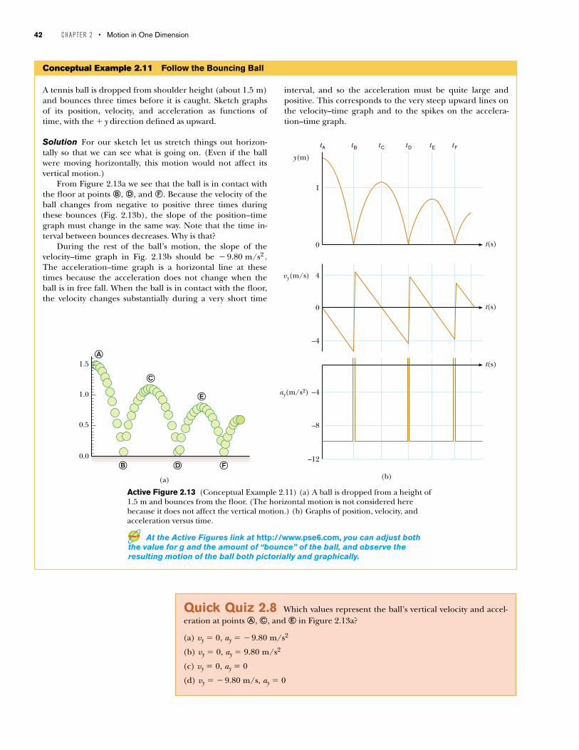
Conceptual Example 2.11 Follow the Bouncing Ball

A tennis ball is dropped from shoulder height (about 1.5 m)and bounces three times before it is caught. Sketch graphsof its position, velocity, and acceleration as functions oftime, with the % y direction defined as upward.

Solution For our sketch let us stretch things out horizon-tally so that we can see what is going on. (Even if the ballwere moving horizontally, this motion would not affect itsvertical motion.)

From Figure 2.13a we see that the ball is in contact withthe floor at points ", $, and &. Because the velocity of theball changes from negative to positive three times duringthese bounces (Fig. 2.13b), the slope of the position–timegraph must change in the same way. Note that the time in-terval between bounces decreases. Why is that?

During the rest of the ball’s motion, the slope of the velocity–time graph in Fig. 2.13b should be # 9.80 m/s2 .The acceleration–time graph is a horizontal line at thesetimes because the acceleration does not change when theball is in free fall. When the ball is in contact with the floor,the velocity changes substantially during a very short time

interval, and so the acceleration must be quite large andpositive. This corresponds to the very steep upward lines onthe velocity–time graph and to the spikes on the accelera-tion–time graph.

(a)

1.0

0.0

0.5

1.5!

#

%

" $ &

1

0

4

0

–4

–4

–8

–12

tA tB tC tD tE tF

y(m)

vy(m/s)

ay(m/s2)

t(s)

t(s)

t(s)

(b)

Active Figure 2.13 (Conceptual Example 2.11) (a) A ball is dropped from a height of1.5 m and bounces from the floor. (The horizontal motion is not considered herebecause it does not affect the vertical motion.) (b) Graphs of position, velocity, andacceleration versus time.

Quick Quiz 2.8 Which values represent the ball’s vertical velocity and accel-eration at points !, #, and % in Figure 2.13a?

(a) vy ! 0, ay ! # 9.80 m/s2

(b) vy ! 0, ay ! 9.80 m/s2

(c) vy ! 0, ay ! 0

(d) vy ! # 9.80 m/s, ay ! 0

At the Active Figures link at http://www.pse6.com, you can adjust boththe value for g and the amount of “bounce” of the ball, and observe theresulting motion of the ball both pictorially and graphically.

S E C T I O N 2 . 6 • Freely Falling Objects 43

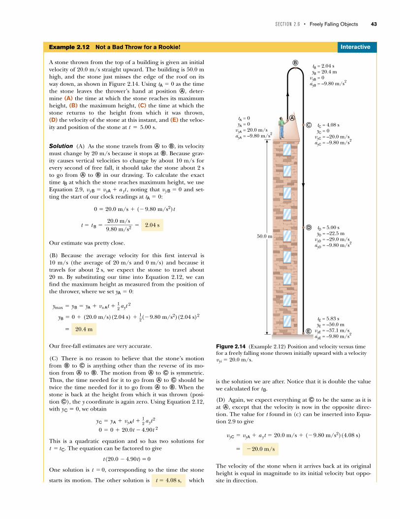
Example 2.12 Not a Bad Throw for a Rookie!

A stone thrown from the top of a building is given an initialvelocity of 20.0 m/s straight upward. The building is 50.0 mhigh, and the stone just misses the edge of the roof on itsway down, as shown in Figure 2.14. Using tA ! 0 as the timethe stone leaves the thrower’s hand at position !, deter-mine (A) the time at which the stone reaches its maximumheight, (B) the maximum height, (C) the time at which thestone returns to the height from which it was thrown, (D) the velocity of the stone at this instant, and (E) the veloc-ity and position of the stone at t ! 5.00 s.

Solution (A) As the stone travels from ! to ", its velocitymust change by 20 m/s because it stops at ". Because grav-ity causes vertical velocities to change by about 10 m/s forevery second of free fall, it should take the stone about 2 sto go from ! to " in our drawing. To calculate the exacttime tB at which the stone reaches maximum height, we useEquation 2.9, vy B ! vyA % a yt , noting that vy B ! 0 and set-ting the start of our clock readings at tA ! 0:

0 ! 20.0 m/s % (# 9.80 m/s2)t

Our estimate was pretty close.

(B) Because the average velocity for this first interval is10 m/s (the average of 20 m/s and 0 m/s) and because ittravels for about 2 s, we expect the stone to travel about20 m. By substituting our time into Equation 2.12, we canfind the maximum height as measured from the position ofthe thrower, where we set yA ! 0:

Our free-fall estimates are very accurate.

(C) There is no reason to believe that the stone’s motionfrom " to # is anything other than the reverse of its mo-tion from ! to ". The motion from ! to # is symmetric.Thus, the time needed for it to go from ! to # should betwice the time needed for it to go from ! to ". When thestone is back at the height from which it was thrown (posi-tion #), the y coordinate is again zero. Using Equation 2.12,with yC ! 0, we obtain

This is a quadratic equation and so has two solutions for t ! tC. The equation can be factored to give

t(20.0 # 4.90t) ! 0

One solution is t ! 0, corresponding to the time the stone

starts its motion. The other solution is which t ! 4.08 s,

0 ! 0 % 20.0t # 4.90t 2

yC ! yA % vy At % 12 ayt2

20.4 m!

yB ! 0 % (20.0 m/s)(2.04 s) % 12(#9.80 m/s2)(2.04 s)2

ymax ! yB ! yA % vx At % 12 ayt 2

2.04 st ! t B !20.0 m/s9.80 m/s2 !

%

$

#

"

!

tD = 5.00 s yD = –22.5 mvyD = –29.0 m/sayD = –9.80 m/s2

tC = 4.08 s yC = 0vyC = –20.0 m/sayC = –9.80 m/s2

tB = 2.04 s yB = 20.4 mvyB = 0ayB = –9.80 m/s2

50.0 m

tE = 5.83 s yE = –50.0 mvyE = –37.1 m/sayE = –9.80 m/s2

tA = 0 yA = 0vyA = 20.0 m/sayA = –9.80 m/s2

!

Figure 2.14 (Example 2.12) Position and velocity versus timefor a freely falling stone thrown initially upward with a velocityvyi ! 20.0 m/s.

is the solution we are after. Notice that it is double the valuewe calculated for tB.

(D) Again, we expect everything at # to be the same as it isat !, except that the velocity is now in the opposite direc-tion. The value for t found in (c) can be inserted into Equa-tion 2.9 to give

The velocity of the stone when it arrives back at its originalheight is equal in magnitude to its initial velocity but oppo-site in direction.

#20.0 m/s!

vyC ! vyA % ayt ! 20.0 m/s % (#9.80 m/s2)(4.08 s)

Interactive

position of the stone at tD ! 5.00 s (with respect to tA ! 0)by defining a new initial instant, tC ! 0:

What If? What if the building were 30.0 m tall instead of50.0 m tall? Which answers in parts (A) to (E) wouldchange?

Answer None of the answers would change. All of themotion takes place in the air, and the stone does not inter-act with the ground during the first 5.00 s. (Notice thateven for a 30.0-m tall building, the stone is above theground at t ! 5.00 s.) Thus, the height of the building isnot an issue. Mathematically, if we look back over our cal-culations, we see that we never entered the height of thebuilding into any equation.

#22.5 m!

% 12 (# 9.80 m/s2)(5.00 s #4.08 s)2

! 0 % (#20.0 m/s)(5.00 s # 4.08 s)

yD ! yC % vy C t % 12 ayt 2

(E) For this part we ignore the first part of the motion(! : ") and consider what happens as the stone falls fromposition ", where it has zero vertical velocity, to position$. We define the initial time as tB ! 0. Because the giventime for this part of the motion relative to our new zero oftime is 5.00 s # 2.04 s ! 2.96 s, we estimate that the acceler-ation due to gravity will have changed the speed by about30 m/s. We can calculate this from Equation 2.9, where wetake t ! 2.96 s:

We could just as easily have made our calculation be-tween positions ! (where we return to our original initialtime tA ! 0) and $:

To further demonstrate that we can choose different ini-tial instants of time, let us use Equation 2.12 to find the

! #29.0 m/s

vyD ! vy A % ayt ! 20.0 m/s % (# 9.80 m/s2)(5.00 s)

#29.0 m/s!

vyD ! vy B % ayt ! 0 m/s % (# 9.80 m/s2)(2.96 s)


vx

t

Area = vxn ∆tn

∆t n

t i t f

vxn

Figure 2.15 Velocity versustime for a particle movingalong the x axis. The area ofthe shaded rectangle is equalto the displacement $x in thetime interval $tn , while thetotal area under the curve isthe total displacement of theparticle.

2.7 Kinematic Equations Derived from Calculus

This section assumes the reader is familiar with the techniques of integral calculus.If you have not yet studied integration in your calculus course, you should skip this sec-tion or cover it after you become familiar with integration.

The velocity of a particle moving in a straight line can be obtained if its position asa function of time is known. Mathematically, the velocity equals the derivative of theposition with respect to time. It is also possible to find the position of a particle if its ve-locity is known as a function of time. In calculus, the procedure used to perform thistask is referred to either as integration or as finding the antiderivative. Graphically, it isequivalent to finding the area under a curve.

Suppose the vx -t graph for a particle moving along the x axis is as shown in Figure 2.15. Let us divide the time interval tf # t i into many small intervals, each of

You can study the motion of the thrown ball at the Interactive Worked Example link at http://www.pse6.com.

S E C T I O N 2 . 7 • Kinematic Equations Derived from Calculus 45

duration $tn. From the definition of average velocity we see that the displacement during any small interval, such as the one shaded in Figure 2.15, is given by

where is the average velocity in that interval. Therefore, thedisplacement during this small interval is simply the area of the shaded rectangle. The total displacement for the interval tf # ti is the sum of the areas of all therectangles:

where the symbol + (upper case Greek sigma) signifies a sum over all terms, that is,over all values of n. In this case, the sum is taken over all the rectangles from ti to tf .Now, as the intervals are made smaller and smaller, the number of terms in the sum in-creases and the sum approaches a value equal to the area under the velocity–timegraph. Therefore, in the limit n : ,, or $tn : 0, the displacement is

(2.14)

or

Note that we have replaced the average velocity with the instantaneous velocity vxnin the sum. As you can see from Figure 2.15, this approximation is valid in the limit ofvery small intervals. Therefore if we know the vx -t graph for motion along a straightline, we can obtain the displacement during any time interval by measuring the areaunder the curve corresponding to that time interval.

The limit of the sum shown in Equation 2.14 is called a definite integral and iswritten

(2.15)

where vx(t) denotes the velocity at any time t. If the explicit functional form of vx(t) isknown and the limits are given, then the integral can be evaluated. Sometimes the vx -tgraph for a moving particle has a shape much simpler than that shown in Figure 2.15.For example, suppose a particle moves at a constant velocity vxi. In this case, the vx -tgraph is a horizontal line, as in Figure 2.16, and the displacement of the particle dur-ing the time interval $t is simply the area of the shaded rectangle:

As another example, consider a particle moving with a velocity that is proportional to t,as in Figure 2.17. Taking vx ! axt, where ax is the constant of proportionality (the

$x ! vxi $t (when vx ! vxi ! constant)

lim$tn : 0 %

nvxn $tn ! &tf

tivx(t)dt

vxn

Displacement ! area under the vx-t graph

$x ! lim$tn : 0%

nvxn $tn

$x ! %n

vxn $tn

vxn$xn ! vxn $tn

vx = vxi = constant

t f

vxi

t

∆t

t i

vx

vxi

Figure 2.16 The velocity–time curve for aparticle moving with constant velocity vxi.The displacement of the particle during thetime interval tf # ti is equal to the area of theshaded rectangle.

Definite integral

acceleration), we find that the displacement of the particle during the time intervalt ! 0 to t ! tA is equal to the area of the shaded triangle in Figure 2.17:

Kinematic Equations

We now use the defining equations for acceleration and velocity to derive two of ourkinematic equations, Equations 2.9 and 2.12.

The defining equation for acceleration (Eq. 2.7),

may be written as dvx ! axdt or, in terms of an integral (or antiderivative), as

For the special case in which the acceleration is constant, ax can be removed from theintegral to give

(2.16)

which is Equation 2.9.Now let us consider the defining equation for velocity (Eq. 2.5):

We can write this as dx ! vx dt, or in integral form as

Because vx ! vxf ! vxi % axt, this expression becomes

which is Equation 2.12. Besides what you might expect to learn about physics concepts, a very valu-

able skill you should hope to take away from your physics course is the ability tosolve complicated problems. The way physicists approach complex situationsand break them down into manageable pieces is extremely useful. On the nextpage is a general problem-solving strategy that will help guide you through thesteps. To help you remember the steps of the strategy, they are called Conceptu-alize, Categorize, Analyze, and Finalize.

! vxi t % 12axt2

xf # xi ! &t

0(vxi % axt)dt ! &t

0vxidt % ax&t

0tdt ! vxi(t # 0) % ax" t 2

2# 0#

xf #xi ! &t

0vxdt

vx !dxdt

vxf #vxi ! ax&t

0dt ! ax(t # 0) ! axt

vxf # vxi ! &t

0axdt

ax !dvx

dt

$x ! 12(tA)(axtA) ! 1

2 axtA

2


t

v x = a xt

v x

a xtA

t A

!

Figure 2.17 The velocity–time curve for a parti-cle moving with a velocity that is proportional tothe time.

Analyze

• Now you must analyze the problem and strive for amathematical solution. Because you have already cat-egorized the problem, it should not be too difficult toselect relevant equations that apply to the type of situ-ation in the problem. For example, if the problem in-volves a particle moving under constant acceleration,Equations 2.9 to 2.13 are relevant.

• Use algebra (and calculus, if necessary) to solve sym-bolically for the unknown variable in terms of what isgiven. Substitute in the appropriate numbers, calcu-late the result, and round it to the proper number ofsignificant figures.

Finalize

• This is the most important part. Examine your nu-merical answer. Does it have the correct units? Does itmeet your expectations from your conceptualizationof the problem? What about the algebraic form of theresult—before you substituted numerical values?Does it make sense? Examine the variables in theproblem to see whether the answer would change in aphysically meaningful way if they were drastically in-creased or decreased or even became zero. Lookingat limiting cases to see whether they yield expectedvalues is a very useful way to make sure that you areobtaining reasonable results.

• Think about how this problem compares with othersyou have solved. How was it similar? In what criticalways did it differ? Why was this problem assigned? Youshould have learned something by doing it. Can youfigure out what? If it is a new category of problem, besure you understand it so that you can use it as amodel for solving future problems in the same cate-gory.

When solving complex problems, you may need toidentify a series of sub-problems and apply the problem-solving strategy to each. For very simple problems, youprobably don’t need this strategy at all. But when youare looking at a problem and you don’t know what todo next, remember the steps in the strategy and use themas a guide.

For practice, it would be useful for you to go backover the examples in this chapter and identify the Concep-tualize, Categorize, Analyze, and Finalize steps. In the nextchapter, we will begin to show these steps explicitly in theexamples.

Conceptualize

• The first thing to do when approaching a problem isto think about and understand the situation. Study care-fully any diagrams, graphs, tables, or photographsthat accompany the problem. Imagine a movie, run-ning in your mind, of what happens in the problem.

• If a diagram is not provided, you should almost alwaysmake a quick drawing of the situation. Indicate anyknown values, perhaps in a table or directly on yoursketch.

• Now focus on what algebraic or numerical informa-tion is given in the problem. Carefully read the prob-lem statement, looking for key phrases such as “startsfrom rest” (vi ! 0), “stops” (vf ! 0), or “freely falls”(ay ! # g ! # 9.80 m/s2).

• Now focus on the expected result of solving the prob-lem. Exactly what is the question asking? Will the fi-nal result be numerical or algebraic? Do you knowwhat units to expect?

• Don’t forget to incorporate information from yourown experiences and common sense. What shoulda reasonable answer look like? For example, youwouldn’t expect to calculate the speed of an automo-bile to be 5 " 106 m/s.

Categorize

• Once you have a good idea of what the problem isabout, you need to simplify the problem. Remove thedetails that are not important to the solution. Forexample, model a moving object as a particle. If ap-propriate, ignore air resistance or friction between asliding object and a surface.

• Once the problem is simplified, it is important to cate-gorize the problem. Is it a simple plug-in problem, suchthat numbers can be simply substituted into a defini-tion? If so, the problem is likely to be finished whenthis substitution is done. If not, you face what we cancall an analysis problem—the situation must be ana-lyzed more deeply to reach a solution.

• If it is an analysis problem, it needs to be categorizedfurther. Have you seen this type of problem before?Does it fall into the growing list of types of problemsthat you have solved previously? Being able to classifya problem can make it much easier to lay out a planto solve it. For example, if your simplification showsthat the problem can be treated as a particle movingunder constant acceleration and you have alreadysolved such a problem (such as the examples in Sec-tion 2.5), the solution to the present problem followsa similar pattern.

G E N E RAL PROB LE M-SOLVI NG STRATEGY

47


After a particle moves along the x axis from some initial position xi to some final posi-tion xf , its displacement is

(2.1)

The average velocity of a particle during some time interval is the displacement$x divided by the time interval $t during which that displacement occurs:

(2.2)

The average speed of a particle is equal to the ratio of the total distance it travelsto the total time interval during which it travels that distance:

(2.3)

The instantaneous velocity of a particle is defined as the limit of the ratio $x/$tas $t approaches zero. By definition, this limit equals the derivative of x with respect tot, or the time rate of change of the position:

(2.5)

The instantaneous speed of a particle is equal to the magnitude of its instantaneousvelocity.

The average acceleration of a particle is defined as the ratio of the change in itsvelocity $vx divided by the time interval $t during which that change occurs:

(2.6)

The instantaneous acceleration is equal to the limit of the ratio $vx /$t as $t ap-proaches 0. By definition, this limit equals the derivative of vx with respect to t, or thetime rate of change of the velocity:

(2.7)

When the object’s velocity and acceleration are in the same direction, the object isspeeding up. On the other hand, when the object’s velocity and acceleration are in op-posite directions, the object is slowing down. Remembering that F a is a useful way toidentify the direction of the acceleration.

The equations of kinematics for a particle moving along the x axis with uniformacceleration ax (constant in magnitude and direction) are

(2.9)

(2.11)

(2.12)

(2.13)

An object falling freely in the presence of the Earth’s gravity experiences a free-fallacceleration directed toward the center of the Earth. If air resistance is neglected, ifthe motion occurs near the surface of the Earth, and if the range of the motion issmall compared with the Earth’s radius, then the free-fall acceleration g is constantover the range of motion, where g is equal to 9.80 m/s2.

Complicated problems are best approached in an organized manner. You shouldbe able to recall and apply the Conceptualize, Categorize, Analyze, and Finalize steps of theGeneral Problem-Solving Strategy when you need them.

vxf2 ! vxi

2 % 2ax(xf # xi)

xf ! xi % vxit % 12axt 2

xf ! xi % vxt ! xi % 12(vxi % vxf)t

vxf ! vxi % axt

)

ax ! lim$t : 0

$vx

$t!

dvx

dt

ax ! $vx

$t!

vxf # vxi

tf # ti

vx ! lim$t : 0

$x$t

!dxdt

Average speed !total distance

total time

vx ! $x$t

$x ! xf # xi

S U M M A RY

Take a practice test forthis chapter by clicking thePractice Test link athttp://www.pse6.com.

Problems 49

1. The speed of sound in air is 331 m/s. During the nextthunderstorm, try to estimate your distance from a light-ning bolt by measuring the time lag between the flash andthe thunderclap. You can ignore the time it takes for thelight flash to reach you. Why?

2. The average velocity of a particle moving in one dimen-sion has a positive value. Is it possible for the instanta-neous velocity to have been negative at any time in the in-terval? Suppose the particle started at the origin x ! 0. Ifits average velocity is positive, could the particle ever havebeen in the # x region of the axis?

If the average velocity of an object is zero in some time in-terval, what can you say about the displacement of the ob-ject for that interval?

4. Can the instantaneous velocity of an object at an instant oftime ever be greater in magnitude than the average veloc-ity over a time interval containing the instant? Can it everbe less?

5. If an object’s average velocity is nonzero over some timeinterval, does this mean that its instantaneous velocity isnever zero during the interval? Explain your answer.

6. If an object’s average velocity is zero over some time inter-val, show that its instantaneous velocity must be zero atsome time during the interval. It may be useful in yourproof to sketch a graph of x versus t and to note that vx(t )is a continuous function.

7. If the velocity of a particle is nonzero, can its accelerationbe zero? Explain.

8. If the velocity of a particle is zero, can its acceleration benonzero? Explain.

Two cars are moving in the same direction in parallel lanesalong a highway. At some instant, the velocity of car A ex-ceeds the velocity of car B. Does this mean that the acceler-ation of A is greater than that of B? Explain.

10. Is it possible for the velocity and the acceleration of an ob-ject to have opposite signs? If not, state a proof. If so, givean example of such a situation and sketch a velocity–timegraph to prove your point.

Consider the following combinations of signs and valuesfor velocity and acceleration of a particle with respect to aone-dimensional x axis:

11.

9.

3.

Velocity Acceleration

a. Positive Positiveb. Positive Negativec. Positive Zerod. Negative Positivee. Negative Negativef. Negative Zerog. Zero Positiveh. Zero Negative

Describe what a particle is doing in each case, and give areal life example for an automobile on an east-west one-di-mensional axis, with east considered the positive direction.

12. Can the equations of kinematics (Eqs. 2.9–2.13) be used ina situation where the acceleration varies in time? Can theybe used when the acceleration is zero?

13. A stone is thrown vertically upward from the roof of abuilding. Does the position of the stone depend on the lo-cation chosen for the origin of the coordinate system?Does the stone’s velocity depend on the choice of origin?Explain your answers.

14. A child throws a marble into the air with an initial speed vi.Another child drops a ball at the same instant. Comparethe accelerations of the two objects while they are in flight.

A student at the top of a building of height h throws one ballupward with a speed of vi and then throws a second balldownward with the same initial speed, vi . How do the finalvelocities of the balls compare when they reach the ground?

16. An object falls freely from height h. It is released at timezero and strikes the ground at time t. (a) When the objectis at height 0.5h, is the time earlier than 0.5t, equal to 0.5t,or later than 0.5t? (b) When the time is 0.5t, is the heightof the object greater than 0.5h, equal to 0.5h, or less than0.5h? Give reasons for your answers.

17. You drop a ball from a window on an upper floor of a build-ing. It strikes the ground with speed v. You now repeat thedrop, but you have a friend down on the street who throwsanother ball upward at speed v. Your friend throws the ballupward at exactly the same time that you drop yours fromthe window. At some location, the balls pass each other. Isthis location at the halfway point between window andground, above this point, or below this point?

15.

Q U E S T I O N S

Section 2.1 Position, Velocity, and Speed

1. The position of a pinewood derby car was observed at vari-ous times; the results are summarized in the followingtable. Find the average velocity of the car for (a) the first

second, (b) the last 3 s, and (c) the entire period of obser-vation.

t(s) 0 1.0 2.0 3.0 4.0 5.0

x(m) 0 2.3 9.2 20.7 36.8 57.5

1, 2, 3 = straightforward, intermediate, challenging = full solution available in the Student Solutions Manual and Study Guide

= coached solution with hints available at http://www.pse6.com = computer useful in solving problem

= paired numerical and symbolic problems

P R O B L E M S


2. (a) Sand dunes in a desert move over time as sand is sweptup the windward side to settle in the lee side. Such “walk-ing” dunes have been known to walk 20 feet in a year andcan travel as much as 100 feet per year in particularlywindy times. Calculate the average speed in each case inm/s. (b) Fingernails grow at the rate of drifting conti-nents, on the order of 10 mm/yr. Approximately how longdid it take for North America to separate from Europe, adistance of about 3 000 mi?

The position versus time for a certain particle movingalong the x axis is shown in Figure P2.3. Find the averagevelocity in the time intervals (a) 0 to 2 s, (b) 0 to 4 s,(c) 2 s to 4 s, (d) 4 s to 7 s, (e) 0 to 8 s.

3.

4. A particle moves according to the equation x ! 10t 2 wherex is in meters and t is in seconds. (a) Find the average veloc-ity for the time interval from 2.00 s to 3.00 s. (b) Find theaverage velocity for the time interval from 2.00 to 2.10 s.

A person walks first at a constant speed of 5.00 m/s alonga straight line from point A to point B and then backalong the line from B to A at a constant speed of 3.00 m/s.What is (a) her average speed over the entire trip? (b) heraverage velocity over the entire trip?

Section 2.2 Instantaneous Velocity and Speed6. The position of a particle moving along the x axis varies in

time according to the expression x ! 3t 2, where x is in me-ters and t is in seconds. Evaluate its position (a) at t ! 3.00 sand (b) at 3.00 s % $t. (c) Evaluate the limit of $x/$t as $tapproaches zero, to find the velocity at t ! 3.00 s.

A position-time graph for a particle moving along thex axis is shown in Figure P2.7. (a) Find the average veloc-ity in the time interval t ! 1.50 s to t ! 4.00 s. (b) Deter-mine the instantaneous velocity at t ! 2.00 s by measuringthe slope of the tangent line shown in the graph. (c) Atwhat value of t is the velocity zero?

8. (a) Use the data in Problem 1 to construct a smooth graphof position versus time. (b) By constructing tangents to thex(t) curve, find the instantaneous velocity of the car at sev-eral instants. (c) Plot the instantaneous velocity versus timeand, from this, determine the average acceleration of thecar. (d) What was the initial velocity of the car?

7.

5.

9. Find the instantaneous velocity of the particle describedin Figure P2.3 at the following times: (a) t ! 1.0 s,(b) t ! 3.0 s, (c) t ! 4.5 s, and (d) t ! 7.5 s.

10. A hare and a tortoise compete in a race over a course1.00 km long. The tortoise crawls straight and steadily atits maximum speed of 0.200 m/s toward the finish line.The hare runs at its maximum speed of 8.00 m/s towardthe goal for 0.800 km and then stops to tease the tortoise.How close to the goal can the hare let the tortoise ap-proach before resuming the race, which the tortoise winsin a photo finish? Assume that, when moving, both ani-mals move steadily at their respective maximum speeds.

Section 2.3 Acceleration

11. A 50.0-g superball traveling at 25.0 m/s bounces off a brick wall and rebounds at 22.0 m/s. A high-speed camerarecords this event. If the ball is in contact with the wall for3.50 ms, what is the magnitude of the average accelerationof the ball during this time interval? (Note: 1 ms ! 10#3 s.)

12. A particle starts from rest and accelerates as shown inFigure P2.12. Determine (a) the particle’s speed at t !

10.0 s and at t ! 20.0 s, and (b) the distance traveled inthe first 20.0 s.

1 2 3 4 5 6 7 8t(s)

–6

–4

–2

0

2

4

6

8

10

x(m)

10

12

6

8

2

4

0t(s)

x(m)

1 2 3 4 5 6

2

ax(m/s2)

0

1

–3

–2

5 10 15 20t(s)

–1

Figure P2.3 Problems 3 and 9

Figure P2.12

Figure P2.7

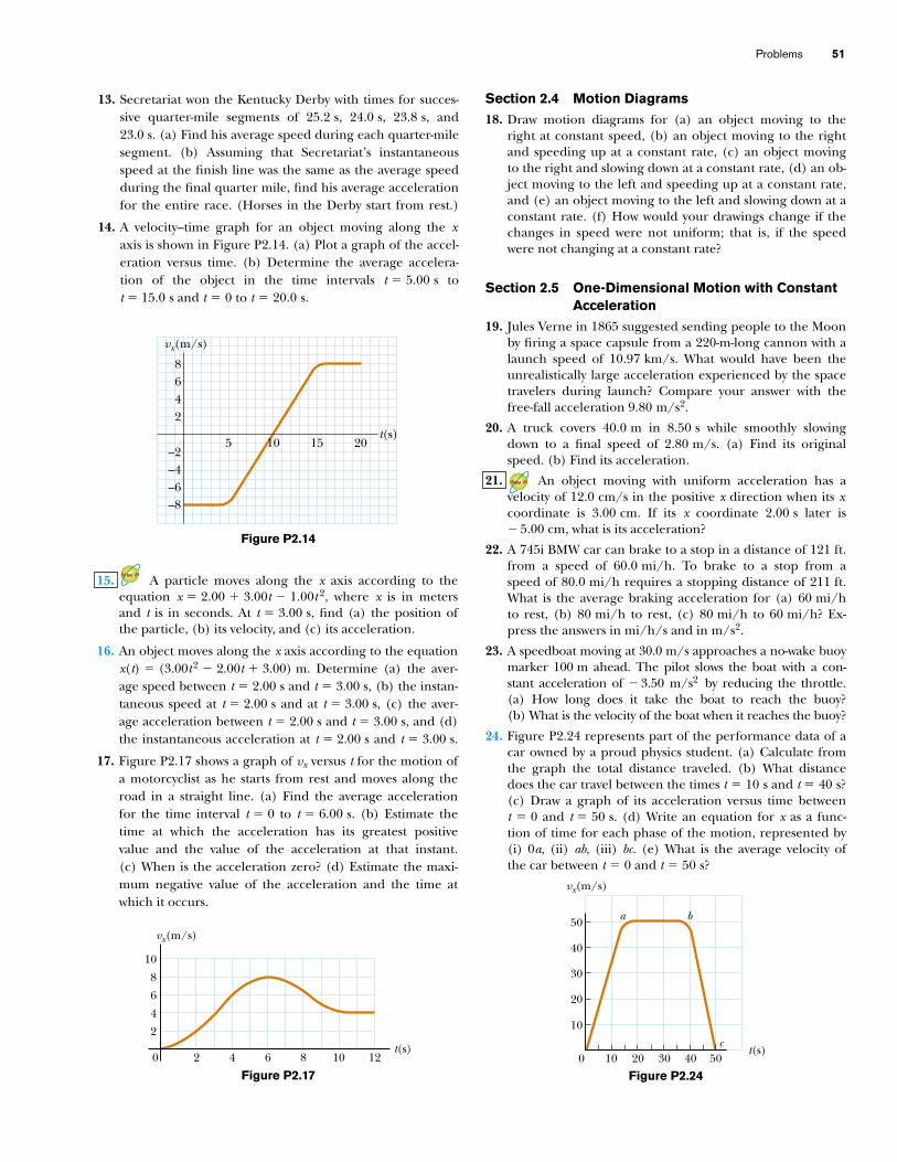
Problems 51

13. Secretariat won the Kentucky Derby with times for succes-sive quarter-mile segments of 25.2 s, 24.0 s, 23.8 s, and23.0 s. (a) Find his average speed during each quarter-milesegment. (b) Assuming that Secretariat’s instantaneousspeed at the finish line was the same as the average speedduring the final quarter mile, find his average accelerationfor the entire race. (Horses in the Derby start from rest.)

14. A velocity–time graph for an object moving along the xaxis is shown in Figure P2.14. (a) Plot a graph of the accel-eration versus time. (b) Determine the average accelera-tion of the object in the time intervals t ! 5.00 s tot ! 15.0 s and t ! 0 to t ! 20.0 s.

A particle moves along the x axis according to theequation x ! 2.00 % 3.00t # 1.00t 2, where x is in metersand t is in seconds. At t ! 3.00 s, find (a) the position ofthe particle, (b) its velocity, and (c) its acceleration.

16. An object moves along the x axis according to the equationx(t) ! (3.00t2 # 2.00t % 3.00) m. Determine (a) the aver-age speed between t ! 2.00 s and t ! 3.00 s, (b) the instan-taneous speed at t ! 2.00 s and at t ! 3.00 s, (c) the aver-age acceleration between t ! 2.00 s and t ! 3.00 s, and (d)the instantaneous acceleration at t ! 2.00 s and t ! 3.00 s.

17. Figure P2.17 shows a graph of vx versus t for the motion ofa motorcyclist as he starts from rest and moves along theroad in a straight line. (a) Find the average accelerationfor the time interval t ! 0 to t ! 6.00 s. (b) Estimate thetime at which the acceleration has its greatest positivevalue and the value of the acceleration at that instant.(c) When is the acceleration zero? (d) Estimate the maxi-mum negative value of the acceleration and the time atwhich it occurs.

15.

Section 2.4 Motion Diagrams18. Draw motion diagrams for (a) an object moving to the

right at constant speed, (b) an object moving to the rightand speeding up at a constant rate, (c) an object movingto the right and slowing down at a constant rate, (d) an ob-ject moving to the left and speeding up at a constant rate,and (e) an object moving to the left and slowing down at aconstant rate. (f) How would your drawings change if thechanges in speed were not uniform; that is, if the speedwere not changing at a constant rate?

Section 2.5 One-Dimensional Motion with ConstantAcceleration

19. Jules Verne in 1865 suggested sending people to the Moonby firing a space capsule from a 220-m-long cannon with alaunch speed of 10.97 km/s. What would have been theunrealistically large acceleration experienced by the spacetravelers during launch? Compare your answer with thefree-fall acceleration 9.80 m/s2.

20. A truck covers 40.0 m in 8.50 s while smoothly slowingdown to a final speed of 2.80 m/s. (a) Find its originalspeed. (b) Find its acceleration.

An object moving with uniform acceleration has a velocity of 12.0 cm/s in the positive x direction when its xcoordinate is 3.00 cm. If its x coordinate 2.00 s later is# 5.00 cm, what is its acceleration?

22. A 745i BMW car can brake to a stop in a distance of 121 ft.from a speed of 60.0 mi/h. To brake to a stop from aspeed of 80.0 mi/h requires a stopping distance of 211 ft.What is the average braking acceleration for (a) 60 mi/hto rest, (b) 80 mi/h to rest, (c) 80 mi/h to 60 mi/h? Ex-press the answers in mi/h/s and in m/s2.

23. A speedboat moving at 30.0 m/s approaches a no-wake buoymarker 100 m ahead. The pilot slows the boat with a con-stant acceleration of # 3.50 m/s2 by reducing the throttle.(a) How long does it take the boat to reach the buoy?(b) What is the velocity of the boat when it reaches the buoy?

24. Figure P2.24 represents part of the performance data of acar owned by a proud physics student. (a) Calculate fromthe graph the total distance traveled. (b) What distancedoes the car travel between the times t ! 10 s and t ! 40 s?(c) Draw a graph of its acceleration versus time betweent ! 0 and t ! 50 s. (d) Write an equation for x as a func-tion of time for each phase of the motion, represented by(i) 0a, (ii) ab, (iii) bc. (e) What is the average velocity ofthe car between t ! 0 and t ! 50 s?

21.

5t(s)

68

24

–4–2

–8–6

10 15 20

vx(m/s)

0 2 4 6 108 12t(s)

2468

10

vx(m/s)

t(s)

vx(m/s)

a b

c50403020100

10

20

30

40

50

Figure P2.14

Figure P2.17 Figure P2.24

25. A particle moves along the x axis. Its position is given by theequation x ! 2 % 3t # 4t 2 with x in meters and t in seconds.Determine (a) its position when it changes direction and(b) its velocity when it returns to the position it had at t ! 0.

26. In the Daytona 500 auto race, a Ford Thunderbird and aMercedes Benz are moving side by side down a straight-away at 71.5 m/s. The driver of the Thunderbird realizeshe must make a pit stop, and he smoothly slows to a stopover a distance of 250 m. He spends 5.00 s in the pit andthen accelerates out, reaching his previous speed of71.5 m/s after a distance of 350 m. At this point, how farhas the Thunderbird fallen behind the Mercedes Benz,which has continued at a constant speed?

A jet plane lands with a speed of 100 m/s and can acceler-ate at a maximum rate of # 5.00 m/s2 as it comes to rest.(a) From the instant the plane touches the runway, what isthe minimum time interval needed before it can come torest? (b) Can this plane land on a small tropical island air-port where the runway is 0.800 km long?

28. A car is approaching a hill at 30.0 m/s when its enginesuddenly fails just at the bottom of the hill. The car moveswith a constant acceleration of # 2.00 m/s2 while coastingup the hill. (a) Write equations for the position along theslope and for the velocity as functions of time, taking x ! 0at the bottom of the hill, where vi ! 30.0 m/s. (b) Deter-mine the maximum distance the car rolls up the hill.

29. The driver of a car slams on the brakes when he sees a treeblocking the road. The car slows uniformly with an acceler-ation of # 5.60 m/s2 for 4.20 s, making straight skid marks62.4 m long ending at the tree. With what speed does thecar then strike the tree?

30. Help! One of our equations is missing! We describe constant-acceleration motion with the variables and parameters vxi ,vxf , ax , t , and xf # x i . Of the equations in Table 2.2, the firstdoes not involve xf # x i . The second does not contain ax ;the third omits vxf and the last leaves out t. So to completethe set there should be an equation not involving vxi . Deriveit from the others. Use it to solve Problem 29 in one step.

For many years Colonel John P. Stapp, USAF, held theworld’s land speed record. On March 19, 1954, he rode arocket-propelled sled that moved down a track at a speedof 632 mi/h. He and the sled were safely brought to rest in1.40 s (Fig. P2.31). Determine (a) the negative accelera-tion he experienced and (b) the distance he traveled dur-ing this negative acceleration.

31.

27.

32. A truck on a straight road starts from rest, accelerating at2.00 m/s2 until it reaches a speed of 20.0 m/s. Then thetruck travels for 20.0 s at constant speed until the brakes areapplied, stopping the truck in a uniform manner in an addi-tional 5.00 s. (a) How long is the truck in motion? (b) Whatis the average velocity of the truck for the motion described?

33. An electron in a cathode ray tube (CRT) accelerates from2.00 " 104 m/s to 6.00 " 106 m/s over 1.50 cm. (a) Howlong does the electron take to travel this 1.50 cm?(b) What is its acceleration?

34. In a 100-m linear accelerator, an electron is accelerated to1.00% of the speed of light in 40.0 m before it coasts for 60.0 m to a target. (a) What is the electron’s acceleration dur-ing the first 40.0 m? (b) How long does the total flight take?

35. Within a complex machine such as a robotic assembly line,suppose that one particular part glides along a straighttrack. A control system measures the average velocity of thepart during each successive interval of time $t0 ! t0 # 0,compares it with the value vc it should be, and switches aservo motor on and off to give the part a correcting pulseof acceleration. The pulse consists of a constant accelera-tion am applied for time interval $tm ! tm # 0 within thenext control time interval $t0. As shown in Fig. P2.35, thepart may be modeled as having zero acceleration when themotor is off (between tm and t0). A computer in the controlsystem chooses the size of the acceleration so that the finalvelocity of the part will have the correct value vc . Assumethe part is initially at rest and is to have instantaneous veloc-ity vc at time t0. (a) Find the required value of am in termsof vc and tm . (b) Show that the displacement $x of the partduring the time interval $t0 is given by $x ! vc (t0 # 0.5tm).For specified values of vc and t0, (c) what is the minimumdisplacement of the part? (d) What is the maximum dis-placement of the part? (e) Are both the minimum andmaximum displacements physically attainable?


t

a

0 t0

am

tm

Figure P2.31 (Left) Col. John Stapp on rocket sled. (Right) Col. Stapp’s face is contorted by thestress of rapid negative acceleration.

Figure P2.35

Cour

tesy

U.S

. Air

Forc

e

Phot

ri, In

c.

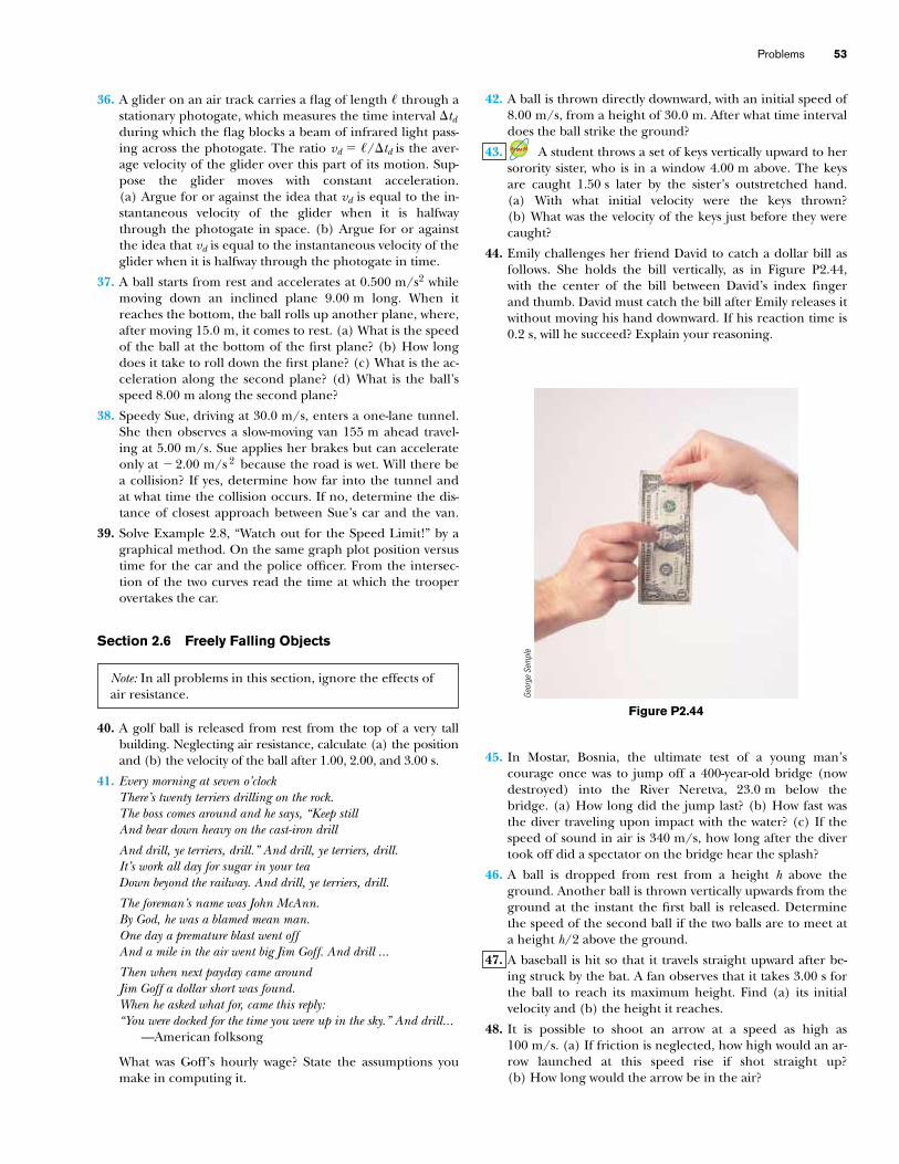
Problems 53

36. A glider on an air track carries a flag of length ! through astationary photogate, which measures the time interval $tdduring which the flag blocks a beam of infrared light pass-ing across the photogate. The ratio vd ! !/$td is the aver-age velocity of the glider over this part of its motion. Sup-pose the glider moves with constant acceleration.(a) Argue for or against the idea that vd is equal to the in-stantaneous velocity of the glider when it is halfwaythrough the photogate in space. (b) Argue for or againstthe idea that vd is equal to the instantaneous velocity of theglider when it is halfway through the photogate in time.

37. A ball starts from rest and accelerates at 0.500 m/s2 whilemoving down an inclined plane 9.00 m long. When itreaches the bottom, the ball rolls up another plane, where,after moving 15.0 m, it comes to rest. (a) What is the speedof the ball at the bottom of the first plane? (b) How longdoes it take to roll down the first plane? (c) What is the ac-celeration along the second plane? (d) What is the ball’sspeed 8.00 m along the second plane?

38. Speedy Sue, driving at 30.0 m/s, enters a one-lane tunnel.She then observes a slow-moving van 155 m ahead travel-ing at 5.00 m/s. Sue applies her brakes but can accelerateonly at # 2.00 m/s 2 because the road is wet. Will there bea collision? If yes, determine how far into the tunnel andat what time the collision occurs. If no, determine the dis-tance of closest approach between Sue’s car and the van.

39. Solve Example 2.8, “Watch out for the Speed Limit!” by agraphical method. On the same graph plot position versustime for the car and the police officer. From the intersec-tion of the two curves read the time at which the trooperovertakes the car.

Section 2.6 Freely Falling Objects

Note: In all problems in this section, ignore the effects ofair resistance.

40. A golf ball is released from rest from the top of a very tallbuilding. Neglecting air resistance, calculate (a) the positionand (b) the velocity of the ball after 1.00, 2.00, and 3.00 s.

41. Every morning at seven o’clockThere’s twenty terriers drilling on the rock.The boss comes around and he says, “Keep stillAnd bear down heavy on the cast-iron drill

And drill, ye terriers, drill.” And drill, ye terriers, drill.It’s work all day for sugar in your teaDown beyond the railway. And drill, ye terriers, drill.

The foreman’s name was John McAnn.By God, he was a blamed mean man.One day a premature blast went offAnd a mile in the air went big Jim Goff. And drill ...

Then when next payday came aroundJim Goff a dollar short was found.When he asked what for, came this reply:“You were docked for the time you were up in the sky.” And drill...

—American folksong

What was Goff’s hourly wage? State the assumptions youmake in computing it.

42. A ball is thrown directly downward, with an initial speed of8.00 m/s, from a height of 30.0 m. After what time intervaldoes the ball strike the ground?

A student throws a set of keys vertically upward to hersorority sister, who is in a window 4.00 m above. The keysare caught 1.50 s later by the sister’s outstretched hand.(a) With what initial velocity were the keys thrown?(b) What was the velocity of the keys just before they werecaught?

44. Emily challenges her friend David to catch a dollar bill asfollows. She holds the bill vertically, as in Figure P2.44,with the center of the bill between David’s index fingerand thumb. David must catch the bill after Emily releases itwithout moving his hand downward. If his reaction time is0.2 s, will he succeed? Explain your reasoning.

43.

45. In Mostar, Bosnia, the ultimate test of a young man’scourage once was to jump off a 400-year-old bridge (nowdestroyed) into the River Neretva, 23.0 m below thebridge. (a) How long did the jump last? (b) How fast wasthe diver traveling upon impact with the water? (c) If thespeed of sound in air is 340 m/s, how long after the divertook off did a spectator on the bridge hear the splash?

46. A ball is dropped from rest from a height h above theground. Another ball is thrown vertically upwards from theground at the instant the first ball is released. Determinethe speed of the second ball if the two balls are to meet ata height h/2 above the ground.

A baseball is hit so that it travels straight upward after be-ing struck by the bat. A fan observes that it takes 3.00 s forthe ball to reach its maximum height. Find (a) its initialvelocity and (b) the height it reaches.

48. It is possible to shoot an arrow at a speed as high as100 m/s. (a) If friction is neglected, how high would an ar-row launched at this speed rise if shot straight up?(b) How long would the arrow be in the air?

47.

Figure P2.44

Geor

ge S

empl

e

A daring ranch hand sitting on a tree limb wishes todrop vertically onto a horse galloping under the tree.The constant speed of the horse is 10.0 m/s, and the dis-tance from the limb to the level of the saddle is 3.00 m.(a) What must be the horizontal distance between thesaddle and limb when the ranch hand makes his move?(b) How long is he in the air?

50. A woman is reported to have fallen 144 ft from the 17thfloor of a building, landing on a metal ventilator box,which she crushed to a depth of 18.0 in. She suffered onlyminor injuries. Neglecting air resistance, calculate (a) thespeed of the woman just before she collided with the venti-lator, (b) her average acceleration while in contact withthe box, and (c) the time it took to crush the box.

51. The height of a helicopter above the ground is given byh ! 3.00t 3, where h is in meters and t is in seconds. After2.00 s, the helicopter releases a small mailbag. How longafter its release does the mailbag reach the ground?

52. A freely falling object requires 1.50 s to travel the last30.0 m before it hits the ground. From what height abovethe ground did it fall?

Section 2.7 Kinematic Equations Derived fromCalculus

Automotive engineers refer to the time rate of change ofacceleration as the “jerk.” If an object moves in one dimen-sion such that its jerk J is constant, (a) determine expres-sions for its acceleration ax(t), velocity vx(t), and positionx(t), given that its initial acceleration, velocity, and posi-tion are axi , vxi , and xi , respectively. (b) Show that

.

54. A student drives a moped along a straight road as de-scribed by the velocity-versus-time graph in Figure P2.54.Sketch this graph in the middle of a sheet of graph paper.(a) Directly above your graph, sketch a graph of the posi-tion versus time, aligning the time coordinates of the twographs. (b) Sketch a graph of the acceleration versus timedirectly below the vx-t graph, again aligning the time coor-dinates. On each graph, show the numerical values of xand ax for all points of inflection. (c) What is the accelera-tion at t ! 6 s? (d) Find the position (relative to the start-ing point) at t ! 6 s. (e) What is the moped’s final positionat t ! 9 s?

axi2 % 2J(vx # vxi)

ax2 !

53.

49. 55. The speed of a bullet as it travels down the barrel of arifle toward the opening is given by v ! (# 5.00 " 107)t 2 %(3.00 " 105)t, where v is in meters per second and t is inseconds. The acceleration of the bullet just as it leaves thebarrel is zero. (a) Determine the acceleration and positionof the bullet as a function of time when the bullet is in thebarrel. (b) Determine the length of time the bullet is ac-celerated. (c) Find the speed at which the bullet leaves thebarrel. (d) What is the length of the barrel?

56. The acceleration of a marble in a certain fluid is propor-tional to the speed of the marble squared, and is given (inSI units) by a ! # 3.00v 2 for v & 0. If the marble entersthis fluid with a speed of 1.50 m/s, how long will it take be-fore the marble’s speed is reduced to half of its initialvalue?

Additional Problems57. A car has an initial velocity v0 when the driver sees an ob-

stacle in the road in front of him. His reaction time is $tr ,and the braking acceleration of the car is a. Show that thetotal stopping distance is

Remember that a is a negative number.

58. The yellow caution light on a traffic signal should stay onlong enough to allow a driver to either pass through theintersection or safely stop before reaching the intersec-tion. A car can stop if its distance from the intersection isgreater than the stopping distance found in the previousproblem. If the car is less than this stopping distance fromthe intersection, the yellow light should stay on longenough to allow the car to pass entirely through the inter-section. (a) Show that the yellow light should stay on for atime interval

where $tr is the driver’s reaction time, v0 is the velocity ofthe car approaching the light at the speed limit, a is thebraking acceleration, and si is the width of the intersec-tion. (b) As city traffic planner, you expect cars toapproach an intersection 16.0 m wide with a speed of60.0 km/h. Be cautious and assume a reaction timeof 1.10 s to allow for a driver’s indecision. Find the lengthof time the yellow light should remain on. Use a brakingacceleration of # 2.00 m/s2.

59. The Acela is the Porsche of American trains. Shown inFigure P2.59a, the electric train whose name is pronouncedah-SELL-ah is in service on the Washington-New York-Boston run. With two power cars and six coaches, it cancarry 304 passengers at 170 mi/h. The carriages tilt as muchas 6- from the vertical to prevent passengers from feelingpushed to the side as they go around curves. Its brakingmechanism uses electric generators to recover its energy ofmotion. A velocity-time graph for the Acela is shown in Fig-ure P2.59b. (a) Describe the motion of the train in each suc-cessive time interval. (b) Find the peak positive accelerationof the train in the motion graphed. (c) Find the train’s dis-placement in miles between t ! 0 and t ! 200 s.

$t light ! $t r # (v0/2a) % (si /v0)

sstop ! v0 $tr # v0

2/2a.


4

vx(m/s)8

–2

2

–6–4

1 2 3 4 5 6t(s)

7 8 9 10

–8

6

Figure P2.54

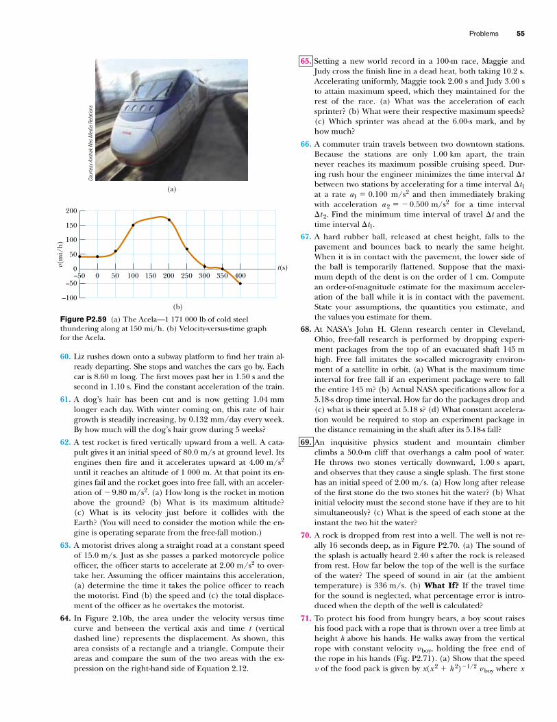
Problems 55

60. Liz rushes down onto a subway platform to find her train al-ready departing. She stops and watches the cars go by. Eachcar is 8.60 m long. The first moves past her in 1.50 s and thesecond in 1.10 s. Find the constant acceleration of the train.

61. A dog’s hair has been cut and is now getting 1.04 mmlonger each day. With winter coming on, this rate of hairgrowth is steadily increasing, by 0.132 mm/day every week.By how much will the dog’s hair grow during 5 weeks?

62. A test rocket is fired vertically upward from a well. A cata-pult gives it an initial speed of 80.0 m/s at ground level. Itsengines then fire and it accelerates upward at 4.00 m/s2

until it reaches an altitude of 1 000 m. At that point its en-gines fail and the rocket goes into free fall, with an acceler-ation of # 9.80 m/s2. (a) How long is the rocket in motionabove the ground? (b) What is its maximum altitude?(c) What is its velocity just before it collides with theEarth? (You will need to consider the motion while the en-gine is operating separate from the free-fall motion.)

63. A motorist drives along a straight road at a constant speedof 15.0 m/s. Just as she passes a parked motorcycle policeofficer, the officer starts to accelerate at 2.00 m/s2 to over-take her. Assuming the officer maintains this acceleration,(a) determine the time it takes the police officer to reachthe motorist. Find (b) the speed and (c) the total displace-ment of the officer as he overtakes the motorist.

64. In Figure 2.10b, the area under the velocity versus timecurve and between the vertical axis and time t (verticaldashed line) represents the displacement. As shown, thisarea consists of a rectangle and a triangle. Compute theirareas and compare the sum of the two areas with the ex-pression on the right-hand side of Equation 2.12.

65. Setting a new world record in a 100-m race, Maggie andJudy cross the finish line in a dead heat, both taking 10.2 s.Accelerating uniformly, Maggie took 2.00 s and Judy 3.00 sto attain maximum speed, which they maintained for therest of the race. (a) What was the acceleration of eachsprinter? (b) What were their respective maximum speeds?(c) Which sprinter was ahead at the 6.00-s mark, and byhow much?

66. A commuter train travels between two downtown stations.Because the stations are only 1.00 km apart, the trainnever reaches its maximum possible cruising speed. Dur-ing rush hour the engineer minimizes the time interval $tbetween two stations by accelerating for a time interval $t1at a rate a1 ! 0.100 m/s2 and then immediately brakingwith acceleration a 2 ! # 0.500 m/s2 for a time interval$t 2. Find the minimum time interval of travel $t and thetime interval $t1.

67. A hard rubber ball, released at chest height, falls to thepavement and bounces back to nearly the same height.When it is in contact with the pavement, the lower side ofthe ball is temporarily flattened. Suppose that the maxi-mum depth of the dent is on the order of 1 cm. Computean order-of-magnitude estimate for the maximum acceler-ation of the ball while it is in contact with the pavement.State your assumptions, the quantities you estimate, andthe values you estimate for them.

68. At NASA’s John H. Glenn research center in Cleveland,Ohio, free-fall research is performed by dropping experi-ment packages from the top of an evacuated shaft 145 mhigh. Free fall imitates the so-called microgravity environ-ment of a satellite in orbit. (a) What is the maximum timeinterval for free fall if an experiment package were to fallthe entire 145 m? (b) Actual NASA specifications allow for a5.18-s drop time interval. How far do the packages drop and(c) what is their speed at 5.18 s? (d) What constant accelera-tion would be required to stop an experiment package inthe distance remaining in the shaft after its 5.18-s fall?

An inquisitive physics student and mountain climberclimbs a 50.0-m cliff that overhangs a calm pool of water.He throws two stones vertically downward, 1.00 s apart,and observes that they cause a single splash. The first stonehas an initial speed of 2.00 m/s. (a) How long after releaseof the first stone do the two stones hit the water? (b) Whatinitial velocity must the second stone have if they are to hitsimultaneously? (c) What is the speed of each stone at theinstant the two hit the water?

70. A rock is dropped from rest into a well. The well is not re-ally 16 seconds deep, as in Figure P2.70. (a) The sound ofthe splash is actually heard 2.40 s after the rock is releasedfrom rest. How far below the top of the well is the surfaceof the water? The speed of sound in air (at the ambienttemperature) is 336 m/s. (b) What If? If the travel timefor the sound is neglected, what percentage error is intro-duced when the depth of the well is calculated?

71. To protect his food from hungry bears, a boy scout raiseshis food pack with a rope that is thrown over a tree limb atheight h above his hands. He walks away from the verticalrope with constant velocity vboy, holding the free end ofthe rope in his hands (Fig. P2.71). (a) Show that the speedv of the food pack is given by x(x 2 % h 2)#1/2 v boy where x

69.

(a)

–50

0

50

100

150

200

–100

0 50 100 150 200 250 300 350 400–50

(b)

v(m

i/h)

t(s)

Figure P2.59 (a) The Acela—1 171 000 lb of cold steelthundering along at 150 mi/h. (b) Velocity-versus-time graphfor the Acela.

Cour

tesy

Am

trak N

ec M

edia

Rel

atio

ns

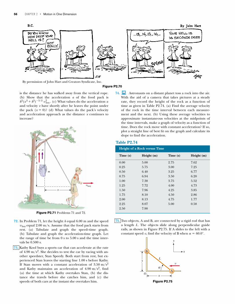
Time (s) Height (m) Time (s) Height (m)

0.00 5.00 2.75 7.620.25 5.75 3.00 7.250.50 6.40 3.25 6.770.75 6.94 3.50 6.201.00 7.38 3.75 5.521.25 7.72 4.00 4.731.50 7.96 4.25 3.851.75 8.10 4.50 2.862.00 8.13 4.75 1.772.25 8.07 5.00 0.582.50 7.90

Height of a Rock versus Time

Table P2.74

is the distance he has walked away from the vertical rope.(b) Show that the acceleration a of the food pack ish2(x 2 % h2)#3/2 v 2

boy . (c) What values do the acceleration aand velocity v have shortly after he leaves the point underthe pack (x ! 0)? (d) What values do the pack’s velocityand acceleration approach as the distance x continues toincrease?

72. In Problem 71, let the height h equal 6.00 m and the speedv boy equal 2.00 m/s. Assume that the food pack starts fromrest. (a) Tabulate and graph the speed–time graph.(b) Tabulate and graph the acceleration-time graph. Letthe range of time be from 0 s to 5.00 s and the time inter-vals be 0.500 s.

Kathy Kool buys a sports car that can accelerate at the rateof 4.90 m/s2. She decides to test the car by racing with an-other speedster, Stan Speedy. Both start from rest, but ex-perienced Stan leaves the starting line 1.00 s before Kathy.If Stan moves with a constant acceleration of 3.50 m/s2

and Kathy maintains an acceleration of 4.90 m/s2, find (a) the time at which Kathy overtakes Stan, (b) the dis-tance she travels before she catches him, and (c) thespeeds of both cars at the instant she overtakes him.

73.

74. Astronauts on a distant planet toss a rock into the air.With the aid of a camera that takes pictures at a steadyrate, they record the height of the rock as a function oftime as given in Table P2.74. (a) Find the average velocityof the rock in the time interval between each measure-ment and the next. (b) Using these average velocities toapproximate instantaneous velocities at the midpoints ofthe time intervals, make a graph of velocity as a function oftime. Does the rock move with constant acceleration? If so,plot a straight line of best fit on the graph and calculate itsslope to find the acceleration.

Two objects, A and B, are connected by a rigid rod that hasa length L. The objects slide along perpendicular guiderails, as shown in Figure P2.75. If A slides to the left with aconstant speed v, find the velocity of B when . ! 60.0°.

75.


m

h

v a

xvboy

α

L

y

x

v

A

B

xO

y

Figure P2.70

Figure P2.71 Problems 71 and 72.

Figure P2.75

By permission of John Hart and Creators Syndicate, Inc.

Answers to Quick Quizzes 57

Answers to Quick Quizzes2.1 (c). If the particle moves along a line without changing di-

rection, the displacement and distance traveled over anytime interval will be the same. As a result, the magnitudeof the average velocity and the average speed will be thesame. If the particle reverses direction, however, the dis-placement will be less than the distance traveled. In turn,the magnitude of the average velocity will be smaller thanthe average speed.

2.2 (b). If the car is slowing down, a force must be pulling inthe direction opposite to its velocity.

2.3 False. Your graph should look something like the follow-ing. This vx -t graph shows that the maximum speed isabout 5.0 m/s, which is 18 km/h (! 11 mi/h), and so thedriver was not speeding.

2.4 (c). If a particle with constant acceleration stops and its ac-celeration remains constant, it must begin to move againin the opposite direction. If it did not, the accelerationwould change from its original constant value to zero.Choice (a) is not correct because the direction of accelera-tion is not specified by the direction of the velocity. Choice(b) is also not correct by counterexample—a car movingin the # x direction and slowing down has a positive accel-eration.

2.5 Graph (a) has a constant slope, indicating a constant accel-eration; this is represented by graph (e).

Graph (b) represents a speed that is increasingconstantly but not at a uniform rate. Thus, theacceleration must be increasing, and the graph that bestindicates this is (d).

Graph (c) depicts a velocity that first increases at aconstant rate, indicating constant acceleration. Then thevelocity stops increasing and becomes constant, indicat-ing zero acceleration. The best match to this situation isgraph (f).

2.6 (e). For the entire time interval that the ball is in free fall,the acceleration is that due to gravity.

2.7 (d). While the ball is rising, it is slowing down. After reach-ing the highest point, the ball begins to fall and its speedincreases.

2.8 (a). At the highest point, the ball is momentarily at rest,but still accelerating at # g.

vx(m/s)

t(s)

6.0

4.0

2.0

0.0

–2.0

–4.0

–6.0

20 30 40 5010

Answer to Quick Quiz 2.3

chapter 2 motion in one dimension - wikispaces this chapter we consider only motion in one...

Documents