chapter 2 molecular - university of alabama

ME 591, Non‐equilibrium gas dynamics, Alexey Volkov 1

Chapter 2 Molecular models

2.1. Degrees of freedom. Molecular models. Simple gas2.2. Model of Hard Sphere (HS) molecules2.3. Interatomic potentials2.4. Mechanics of a binary collisions2.5. Collision cross sections2.6. Variable Hard Sphere (VHS) model

Additional reading:

Sections 1.4, 1.5


2.1. Degrees of freedom. Molecular models. Simple gas Degrees of freedom and energy of molecules Molecular model Simple gas


1.1. Degrees of freedom. Molecular models. Simple gasDegrees of freedom of molecules

In mechanics, the number of degrees of freedom is the number of independent motions thatare allowed to a body or the number of independent parameters that are necessary to describethe position of a body.An atom considered as point mass has 3 translational degrees of freedom (three coordinatesare necessary to described its position).A rigid body has 6 degrees of freedom, 3 coordinates of the center of mass and 3 angles thatdescribe orientation of a body with respect to axis of coordinate system.‐atomic molecule (molecule composed of atoms) has 3 degrees of freedom, since every

atom can move with respect to others. It is convenient to consider the overall motion ofindividual atoms in the molecule as a composition or “superposition” of three types of motion Translational motion of the center of mass of molecules ( 3 translational degrees of

freedom). Rotational motion of molecule as a whole around the center of mass ( 2 or 3

rotational degrees of freedom). Relative or vibrational motion of atoms with respect to each other with

3 3vibrational or internal degrees of freedom.

Both rotational and vibrational degrees of freedom are often called the internal degrees offreedom.


1.1. Degrees of freedom. Molecular models. Simple gasMonatomic molecule (atom): 1, 3, 0, 0.Diatomic molecule: 2, 3, 2, 1.Triatomic molecule: 3, 3, 3, 3.Then the total energy of ‐atomic molecule of mass can be written as

,where /2 is the translational energy, is the energy of rotational degrees offreedom, and is the energy of vibrational degrees of freedom.The importance of the representation of motion of atoms in a molecule in the form ofsuperposition of translational, rotational, and vibrational motions is based on the fact that ,

, and can play different role in collisions. For example, at standard conditions, thevibrational degrees of freedom of N2 and O2 are not excited (i.e., does not change duringcollisions). Then one can neglect in Eq. (2.1.1) and assume that a molecule has 5 degreesof freedom.This approachis routinely used in thermodynamics of diatomic gases.Energy exchange between vibrational and over degrees of freedom can be described only basedon quantum mechanics (vibrational energy is quantized). The translational and often rotationaldegrees of freedom can be satisfactory described by classical mechanics.A collision is called elastic if total translational energy of colliding molecules before and after thecollision does not change, i.e. if there is no energy exchange between translational and otherdegrees of freedom and

′ ′ .

(2.1.1)

We use prime to denote parameters of molecules after a collision


2.1. Degrees of freedom. Molecular models. Simple gasMolecular model

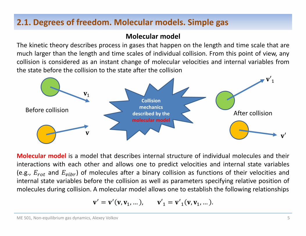
The kinetic theory describes process in gases that happen on the length and time scale that aremuch larger than the length and time scales of individual collision. From this point of view, anycollision is considered as an instant change of molecular velocities and internal variables fromthe state before the collision to the state after the collision

Molecular model is a model that describes internal structure of individual molecules and theirinteractions with each other and allows one to predict velocities and internal state variables(e.g., and ) of molecules after a binary collision as functions of their velocities andinternal state variables before the collision as well as parameters specifying relative position ofmolecules during collision. A molecular model allows one to establish the following relationships

, , … , ′ , , … .

′

′

Before collision After collision

Collision mechanics

described by the molecular model


2.1. Degrees of freedom. Molecular models. Simple gasIn order to establish such relationships, we need to consider in detail the process of individualbinary collision based on a known law of interaction between molecules.

“Simple” gasIn our course, we will consider only molecular models of a “simple” gas, i.e. a gas where allmolecules are identical, and every molecule is considered as a point mass without internalstructure, which does not chance its physical properties under any conditions (no chemicalreactions, ionization, etc.).

In this model, every molecule has only three translation degree of freedom and all binarycollisions are elastic. Interaction forces between molecules then must be Potential or conservative (i.e. they have potential energy; if this is not the case then energy

conservation law cannot be satisfied) and Central (i.e. directed along the line connecting the centers of interacting molecules; if this is

not the case then the angular momentum conservation law cannot be satisfied).

Such model accurately describes properties of monatomic gases composed of individual atoms(noble gases, atomic vapors of various substances), but it can be also used for quantitative (and,sometimes quantitative) studies of gases composed of polyatomic molecules.


2.2. Model of hard sphere (HS) molecules Model of hard sphere (HS) molecules Conservation law during a collision of hard spheres Relationship between velocities before and after collision


2.2. Model of Hard Sphere (HS) moleculesThe model of hard sphere (HS) molecules is the molecular model, when individual moleculesare considered as non‐deformable, non‐rotating spheres of diameter . Binary collision of HSmolecules is assumed to be an instant change of velocities of colliding molecules whenmolecules “touch” each other, i.e. when distance between centers of spheres is equal to .

The state of molecules before the collision is characterized by velocities and , and relativeposition is characterized by the unit vector . Our major goal is to calculate velocities after thecollision ′ and ′ as functions of and , and .We will show that unique values of and can be derived from the conservation lawsassuming instant collision between non‐deformable spheres.

, | | 1

′

′

, Collision at given ′ , ′

Conservation laws during a collision of hard spheresIn closed mechanical systems, linear momentum, angular momentum, and total energyconserve. Let’s write the equations of conservation of these quantities for two states rightbefore and after the collision, when positions of molecules are given by and :

,

,

2 2 2 2 .

In order to simplify these equations let’s introduce the center of mass velocity , relativevelocity , and represent as :

2 , ,

2 , 2 .

Then Eq. (2.2.1) reduces to′ ,

i.e. the center‐of‐mass velocity does not change during the collision. Eq. (2.2.2) reduces to

2 2 2 2 .


2.2. Model of Hard Sphere (HS) molecules

(2.2.1)

(2.2.2)

(2.2.3)

(2.2.6)

(2.2.4)

(2.2.5) This is the consequence of the linear momentum conservation law

HS model describes only elastic collisions

In the last equation, most of terms cancel each other, so it reduces to′ .

2 2 ′′2 ′

′2

or,

i.e. the absolute value of relative velocity does not change during the collision. This is theconsequence of the energy conservation law. Thus, the only result of the collision is thedeflection of the relative velocity vector on angle in the collision plane. The angle is calledthe deflection angle.



(2.2.7)

(2.2.8)

Note that cross product is a vector orthogonal to the plane of vectorsand . Then vectors , , and lye in the same plane. This plane is

called the collisions plane. This is the first consequence of the angularmomentum conservation law. Eq. (2.2.3) reduces to

′ In order to find , let’s introduce normal (along center‐to‐center direction ) and tangential components of vector ,

· ,,

and apply Eq. (2.2.7):

Then combining Eqs. (2.2.9) and (2.2.10) one can obtain

′ ,

′ 2 · .

Eq. (2.2.11) completely describes mechanics of collisionof HS molecules.

or′ .

Now we can multiply the last equation by :.

Using the definition of the cross product, one can prove that for arbitrary vector andorthogonal unit vector the following equation holds: . Thus, the last equationreduces to

′ .

This is the second consequence of Eq. (2.2.2): The tangential component of the relative velocitydoes not change during the collision. Then Eq. (2.2.8) and (2.2.9) show that the only result ofcollisions of HS is the change of the direction of the normal component of the relative velocity:

′ .



(2.2.9)

′(2.2.10)

(2.2.11)

Relative position of molecules during the collision can be defined by the collision parameter (see figure). Then

sin ,

2 2 asin .



′

(2.2.13)

(2.2.12)

(2.2.14)

Relationship between velocities before and after collisionNow we can combine Eqs. (2.2.5), (2.2.6), and (2.2.11) in order to obtain and :

· ,′ · .

In the HS model, the internal structure of molecules is neglected, so that this model is applicableprimarily for collisions of monatomic molecules (noble gases, dissociated oxygen and nitrogen,metal vapors, etc.). Although this model crudely approximates the real process of interactionbetween molecules, it is historically the first and currently one of the most popular models inthe kinetic theory. It is capable of qualitatively description of collisional process in multipleapplications of RGD.The predictions based on the HS model can be often brought in quantitative agreement withmore complicated models and experiments by the appropriate choice of HS diameter .


2.3. Interatomic potentials Interatomic potentials of monatomic gases Lennard‐Jones potential Repulsive potential Morse potential Calculation of forces


2.3. Interatomic potentials

In the case of a monatomic gas, when every molecule is a pointmass that has only translational energy, it is naturally to assumethat the forces between molecules are conservative, i.e.preserve total mechanical energy, and central, i.e. directed alonga line connecting interacting particles.Then, it is shown in mechanics that interaction forces can becompletely defined by the potential energy (often calledinteratomic potential) that depends only on distance betweenmolecules , = , and interaction forces are equal to

,

.

Physical experiments in molecular physics and quantummechanical calculations show that typical dependence of onlooks like shown in the picture. Distance between particleswhen 0 is the equilibrium distance and is thedepth of the potential well.

Interatomic potentials of monatomic gases| |

Force

0 0

Strong repulsion

Weakattraction

We will systematically use this notation for vectors of gradients


2.3. Interatomic potentialsActual dependences of on are complicated or unknown. So for practical purposes, isapproximated by a some simple function. Such approximations are calledmodel potentials.

Lennard‐Jones potentialThe model potential in the form of a difference of two power functions

,where , , , and are given constants, is called the (generalized) Lennard‐Jones potential.The first term describes repulsion at , and the second term describes attraction at .It is shown in quantum mechanics that the van der Waalsattraction is described by the potential that varies as~1/ , so usually 6. Adequate description of therepulsive force requires 11 15, so the averagevalue 12 is often used. For the particular choice of

12 and 6, Eq. (2.3.1) can be re‐written as

2

or

4

/ 2

and called (12‐6) Lennard‐Jones potential or simply Lennard‐Jones potential. In Eqs. (2.3.2) and(2.3.3), is the depth of the potential well and is the equilibrium distance.

(2.3.1)

(2.3.2)

(2.3.3)

Potential

Derivative in reduced units

/

In gas flows without phase changes (e.g.,condensation), the repulsive forces play theprimary role, while the effect of attraction is oftenmarginal. Then one can simplify the molecularmodel given by the Eq. (2.3.1) by neglecting theattraction term and using purely the repulsivepotential

,

where constants and can be chosen to matcha given gas property, usually viscosity, at a giventemperature.The molecular models based on the repulsivepotentials are the most popular models formodelling of monatomic gas flows.


2.3. Interatomic potentialsIn the reduced units, / and / , the Lennard‐Jones potential is unique and we cannotcontrol the width of the potential well.

Repulsive potential

(2.3.4)

/

(12‐6) Lennard‐Jones

Repulsive

4


2.3. Interatomic potentialsMorse potential

The model potential in the form

2 ,where , , and are given constants, is called the Morse potential. In Eq. (2.3.5), is thedepth of the potential well, is the equilibrium distance, and is an additional parameter thatdetermines the bond "rigidity" close to the equilibrium position.

(2.3.5)

The Morse potential has three adjustableparameters that can be used to match threematerial properties known from experiments.Parameter can use used, in particular, inorder to vary the width of the potential well:With increasing , the width of the potentialwell decreases, as illustrated in the figure, andpotential becomes more “stiff” around theequilibrium distance.In the reduced units, / and / , the Morsepotential is defined by the only one parameter

./

4

8

12


2.3. Interatomic potentialsCalculation of forces

,

,

,

,

, , , , , , , .

In mechanics, the potential force exerted on a point mass is equal to the negative gradient of thepotential energy with respect to coordinates of this particle:

,

,

.

i.e. third Newton’s law is automatically satisfied.

(2.3.6)

(2.3.7)

(2.3.8)

Here we use the chain rule

/ is the unit vector directed from molecule 1 to molecule 2


2.4. Mechanics of a binary collision Equations of motion of molecules during a binary collision Conservation laws during a binary collision Equations of relative motion Conservation of angular momentum and collision plane Conservation of total energy Equation of motion in polar coordinates on the collision plane Deflection angle Relationship between velocities before and after collision


2.4. Mechanics of a binary collisionEquations of motion of molecules during a binary collision

The goal of this section is to find post‐collisional velocities after a binary collision of twomolecules (point masses ), if interaction is described by the interatomic potential . Forthis purpose, let's introduce an inertial framework with Cartesian coordinates . In thisframework, state of two interaction molecules at time is defined by the position vectors ,and velocity vectors , . Variation of , , , and along particle trajectories is described theequations of motion that include kinematic relationships between position and velocity vectors,

, and equations of Newton's second law of motion

, ,where and are the interaction forces exertedon molecules 1 and 2. These forces are definedby the interatomic potential | | ,e.g.

.

This system includes 12 scalar equations (3 coordinate and 3 velocity component of individualmolecule x 2 ). We will show that this system of 12 equations can be reduced to a singleequation using the conservation laws!

(2.4.1)

(2.4.2)

Collision plane


2.4. Mechanics of a binary collisionConservation laws during a binary collision

Let's introduce the total linear momentum , angular momentum , andmechanical energy,

,

2 2 | | ,and show that these quantities are conserved during the binary collision:

0.0.

· · · · · · · · 0.

Here is calculated with the chain rule ( , , , , , ):

· · .

Thus, during a binary collision of molecules of monatomic gas the following conservation lawsare valid

,

,

2 2 | | .

(2.4.3)

(2.4.4)

(2.4.5)

Linear momentum c. l.

Angular momentum c. l.

Mechanical energy c. l.

Hereinafter


2.4. Mechanics of a binary collisionEquations of relative motion

In order to simplify Eqs. (2.4.1)‐(2.4.2), let's first use the linear momentum conservation law.Let's introduce the center‐of‐mass velocity position and velocity vectors, as well relativeposition and velocity vectors,

2 , , 2 , .

Then we can write the sum and difference of Eqs (2.4.1) and (2.4.2)

2 2 , ,

2 2 0, .Left pair of equations reduces to equations

, 0that describe the motion of the center of mass and imply that the center of mass moves withconstant velocity . This is the consequence of the linear momentum conservation law, sinceEq. (2.4.4) reduces to 2 . The right pair of equations reduces to equations

, 2that describe relative motion of molecules and can be solved independently of Eqs. (2.4.7).Thus, 12 Eqs. (2.4.1)‐(2.4.2) reduce the system of 6 equations of relative motion.

Linear momentum c. l.

Here we use Eq. (2.3.8)

(2.4.6)

(2.4.7)

(2.4.8)


2.4. Mechanics of a binary collisionConservation of angular momentum and collision plane

Now let's use the angular momentum conservation law and re‐write it in terms of center‐of‐mass and relative motion parameters. The simplest approach to do it is to first find positons andvelocity vectors of individual molecules in terms of , , , and :

2 , 2 , 2 , 2 .Then

2 2 2 2can be reduced to (consider as exercise)

2 2The first term is the angular momentum of the center of mass . It is conserved, since thecenter of mass moves with constant velocity as 0 :

2 2 0 2 0 .

Then during the binary collision the angular momentum of relative motion is also conserved:

2 .

But we know that is a vector normal to the plane of vectors and , and since, during collision and always lye in the same plane that is called the collision

plane. This is the consequence of the angular momentum conservation law.

(2.4.10)

(2.4.11)

(2.4.12)

(2.4.9)


2.4. Mechanics of a binary collision

It means that the trajectory of the relative motion of particles is a planar curve that lies in thecollision plane. Let's introduce a specific Cartesian coordinates that moves together withmolecule 1, where the center coincides with molecule 1 and axis is directed along therelative velocity of molecule 2 with respect to molecule 1 before the collision:

lim→

, .

When the position of the collision plane is characterized by the constant azimuthal angle andthere will be only 4 equations with respect to components of and on the collision plane:

, .

Collision plane

Trajectory of relative motion of molecule 2 with respect to molecule 1

Molecule 1

Relative velocity before the collision



Trajectory on the collision plane


Molecule 1


Relative velocity ′ after the collision

Collisionparameter

(2.4.13)

On the collision plane, relation position of the molecules before the collision can becharacterized by the collision parameter . Then can be found in terms of | | and :

2 lim→

2 lim→

| || | sin , 2 ,

| | 2 .

is the unit vector normal to the collision plane and forming right‐hand triplet , , .


2.4. Mechanics of a binary collisionConservation of energy

Now let's use the mechanical energy conservation law and re‐write it in terms of center‐of‐massand relative motion parameters. Then

2 2 2 2 | | ,can be reduced to (consider as exercise)

22

/22 | | .

The first term, the kinetic energy of the center of mass , is conserved:22 .

Then during the binary collision themechanical energy of relative motion is also conserved:

/22 | | .

If we apply the last equation to the state of molecules before ( → ∞) and after ( → ∞) thecollision, we obtain ( | | → 0 in both cases)

/22

/22 ⟹ ,

i.e., the absolute value of relative velocity before and after the collision is the same. This is themajor consequence of the energy conservation law.

(2.4.14)

(2.4.15)

(2.4.16)


2.4. Mechanics of a binary collisionEquation of motion on the collision plane in polar coordinates

Now let's introduce the polar coordinates , on the collision plane. Then

In order to get differential equations with respect to and let's use Eqs. (2.4.12) and (2.4.14)

2 2 2 ,

2 ,/22 | |

/22 ,

/22 .

Note that in Eqs. (2.4.16) and (2.4.17) and are know constants, since they can becalculated with Eqs. (2.4.13) and (2.4.16) by using only relative velocity and collisionparameter that are supposed to be known. Then we can consider Eqs. (2.4.16) and (2.4.17) as

(2.4.17)

(2.4.18)

cos sin ,

sin cos ,

ξ η ,

.

atan


2.4. Mechanics of a binary collisiondifferential equations with respect to and :

4 4,

2.

In order to find an equation for we need to choose a sign at the square root. Simple analysisshow that the trajectory on the collision plane (see slide 25) is symmetric with respect to theangle that corresponds to approaching of molecules at the minimum distance (so

in slide 25). At , 0,so (but not ) can be found from the equation4 4

.

Then we can replace Eqs. (2.4.18) with

2 , 2

,

where different signs at the square roots corresponds to different branches of the trajectory.Let's consider only the branch where molecules approach each other and 0. If we introduce

, then we can exclude time from the consideration and replace Eq. (2.4.21) withthe only equation that defines :

.

(2.4.19)

(2.4.20)

(2.4.21)

(2.4.22)

This equation predicts trajectory on the collision plane for given and , i.e. for given and , see Eqs. (2.4.13) and (2.4.16)


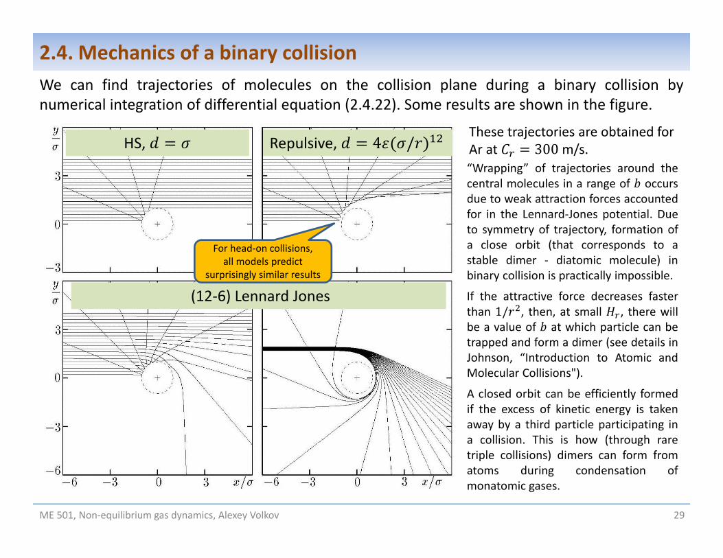
2.4. Mechanics of a binary collisionWe can find trajectories of molecules on the collision plane during a binary collision bynumerical integration of differential equation (2.4.22). Some results are shown in the figure.

These trajectories are obtained for Ar at 300m/s.HS, Repulsive, 4 /

(12‐6) Lennard Jones

“Wrapping” of trajectories around thecentral molecules in a range of occursdue to weak attraction forces accountedfor in the Lennard‐Jones potential. Dueto symmetry of trajectory, formation ofa close orbit (that corresponds to astable dimer ‐ diatomic molecule) inbinary collision is practically impossible.

If the attractive force decreases fasterthan 1/ , then, at small , there willbe a value of at which particle can betrapped and form a dimer (see details inJohnson, “Introduction to Atomic andMolecular Collisions").

A closed orbit can be efficiently formedif the excess of kinetic energy is takenaway by a third particle participating ina collision. This is how (through raretriple collisions) dimers can form fromatoms during condensation ofmonatomic gases.

For head‐on collisions, all models predict

surprisingly similar results


2.4. Mechanics of a binary collisionDeflection angle

The R.H.S. of differential equation (2.4.22) does not depend on , so the equation can beintegrated from the point where 0 and :

.

Angle in slide 25 corresponds to → ∞ (state of the molecules after collision):

, .

Finally, the deflection angle , the angle between relative velocity vectors before and after thecollision), is equal to

, 2 , 2 .

Here , and are defined by and according to Eqs. (2.4.13), (2.4.16), and (2.4.20).Contrary to the HS model, depends on the relative velocity of molecules before the collision.

(2.4.23)

(2.4.24)

Compare with Eq. (2.2.14) for the HS model

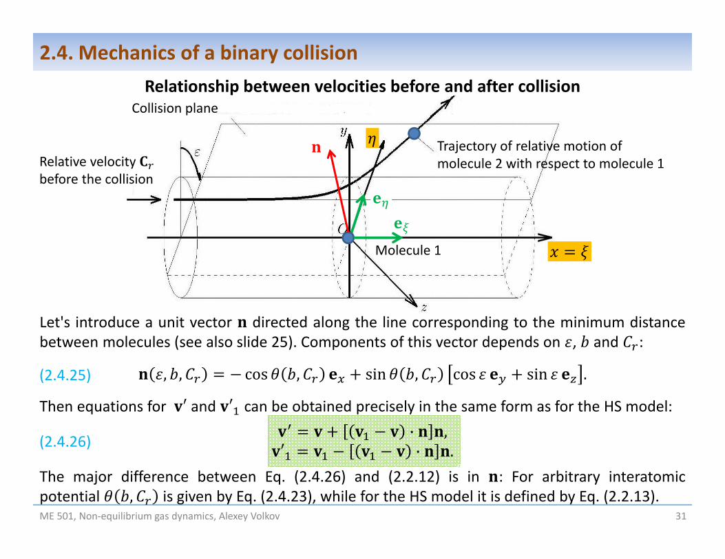
Relationship between velocities before and after collision

Let's introduce a unit vector directed along the line corresponding to the minimum distancebetween molecules (see also slide 25). Components of this vector depends on , and :

, , cos , sin , cos sin .

Then equations for ′ and ′ can be obtained precisely in the same form as for the HS model:· ,

′ · .The major difference between Eq. (2.4.26) and (2.2.12) is in : For arbitrary interatomicpotential , is given by Eq. (2.4.23), while for the HS model it is defined by Eq. (2.2.13).ME 501, Non‐equilibrium gas dynamics, Alexey Volkov 31


(2.4.26)

(2.4.25)

Collision plane


Molecule 1


In order to use Eq. (2.4.26) for practical calculations we need to know how to definecomponents of vector in the global coordinate system, i.e. in the same coordinate system,where we know components of the velocity vectors and . It can be easily done, e.g., if atsome time during collision we know position vectors of molecules and . Then Eq. (2.4.25)can be re‐written as

, , cos , sin , ,

where, according to definition of and collision plane, and can be calculated as follows:

| | , | | , .

Here is a unit vector normal to the collision plane.



(2.4.28)

(2.4.27)


2.5. Collision cross sections Prerequisite: Solid angle Cutoff of interatomic potentials Total collision cross‐section Differential collision cross section Cross sections of HS molecules Scattering


2.5. Collision cross sectionsPrerequisite: Solid angle

Solid angle in 3D space is a volume bounded by a cone withthe vertex in some point .Solid angles are measured by the area Ω that is cut by thecone on the surface of a sphere of unit radius with thecenter in point . Correspondingly, the value of Ω for anybody angle varies from 0 to 4 . It is measured in steradians.

In order to measure various solid angles with the samevertex , it is convenient to use spherical angles:longitudinal angle and co‐latitude :

0 20

A unit vector (direction) that corresponds to given andhas the following components:

, cos sin cos sin .

If we fix some and and give increments and tothese angles, then we obtain a cone (solid angle) of size

Ω sin .

1

Ω

Body angle

(2.5.1)

Ω


2.5. Collision cross sectionsCutoff of interatomic potential

Interatomic potentials introduced in Section 2.3only asymptotically approach zero when → ∞ . Itmeans that the interaction force between moleculesexists at any finite distance, although if is large, thenthe magnitude of the force is so small that there is nopractical reason to take it into account.The use of interatomic potentials with non‐zero forceat any finite distance contradicts the kinetic theory ofdilute gases, which states that only binary collisions areimportant, since then at any time a molecule interactssimultaneously with all other molecules.In order to get rid of this difficulty, cutoff interatomicpotentials are used in practical calculations: It isassumed that is zero if where isthe cutoff distance, i.e. maximum distance betweenmolecules, where forces are non‐zero. Then Eq.(2.4.24) for the deflection angle takes the form

(2.5.2)

Potential

Derivative in reduced units

/

0

Potential /

2 .(2.5.3)

1. Such cutoff implies a jump in the force at. In practical calculations, smooth

cutoff is also applied, when variessmoothly from to 0 in a range

.2. Usually ~ 3 4 .3. There is reason to assume that is not aconstant, but depends on (see section 2.6).

Let's assume that we use only a cutoff interatomic potentialwith the cutoff distance (for the HS model, ). Incalculations of the collision frequency in Section 1.4 wefound that depends on the total collision cross section of HSmolecules. If we want to extend this consideration and countcollisions for molecules interacting via a cutoff potential, thenwe need to assume that the collision cylinder has diameter

. The cross‐sectional area of the collisioncylinder is called the total collision cross section

.Let's assume that we cannot define accurately and thatspecify relative position of molecules before their collision onthe cross section of the collision cylinder. On the contrary, let'sassume that the position is random and position of molecule 2with respect to molecule 1 on the cross section is distributedwith equal probability. Then probability to have a collisionwith

, is equal toME 501, Non‐equilibrium gas dynamics, Alexey Volkov 36

2.5. Collision cross sections

(2.5.4)

(2.5.6)

Total collision cross section

Mesh of cells

∆

Collisioncylinder

(2.5.5)



If is fixed, then the deflection angle is a function of according to Eq. (2.5.3):

, 2 .

It means that if before a collision relative position of molecules satisfies Eq. (2.5.5), then afterthe collision the direction of relative velocity ′ satisfies the equations

, ,where

or, direction of relative velocity ′ is within the body angle Ω sin . The coefficient ofproportionality between area , which corresponds to the relative position ofmolecules on the cross section of collision cylinder before the collision and body angleΩ sin , where the relative velocity of molecules after the collision ′ is directedwithin, is called the differential collision cross section , :

, Ω.If one combines Eqs. (2.5.6) and (2.5.9), then probability to find ′ directed within Ω is

,Ω.

(2.5.9)

(2.5.8)

(2.5.7)

Differential collision cross section

(2.5.10)

Thus, the ratio / defines probability of deflection (scattering) into an infinitely small bodyangle Ω at given value of .

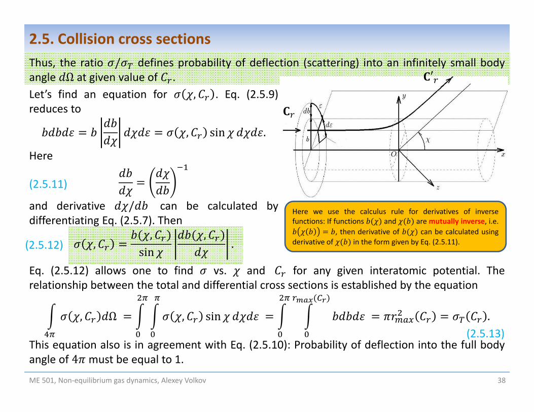
Eq. (2.5.12) allows one to find vs. and for any given interatomic potential. Therelationship between the total and differential cross sections is established by the equation

, Ω , sin .

This equation also is in agreement with Eq. (2.5.10): Probability of deflection into the full bodyangle of 4 must be equal to 1.

Let’s find an equation for , . Eq. (2.5.9)reduces to

, sin .

Here

and derivative / can be calculated bydifferentiating Eq. (2.5.7). Then

,,

sin,

.



(2.5.12)

′

Here we use the calculus rule for derivatives of inversefunctions: If functions and aremutually inverse, i.e.

, then derivative of can be calculated usingderivative of in the form given by Eq. (2.5.11).

(2.5.11)

(2.5.13)


2.5. Collision cross sectionsCross sections of HS molecules

Eq. (2.5.12) can be applied even for HS molecules of diameter d. In this case the relationshipbetween and b is given by Eq. (2.2.14) or

cos 2 ⟹ 2 sin 2 .

Then

4 , Ω 4 4 .

Scattering

(2.5.14)

The problem of calculation of trajectories of relative motion of onemolecule with respect another considered in Sections 2.4 and 2.5 isan example of the general problem in physics and mechanics knownas a problem of elastic particle scattering on the force center.It can be also used to predict gravitational or Coulomb scattering ofparticles of various physical nature in the central fields of gravity orelectrostatic force.In particular, solution of this problem was used by English physicistRutherford to explain experiments on scattering of alpha particlesmoving through a thin gold film. These experiments led to thedevelopment of the planetary Rutherford model of the atom andeventually to the Bohr model.See https://en.wikipedia.org/wiki/Rutherford_scattering.

Fetter and Walecka, "Theoretical Mechanics ofParticles and Continua"


2.6. Variable Hard Sphere (VHS) model Cross sections for the repulsive potential Variable Hard Sphere (VHS) model Parameterization of the VHS model based on the viscosity data


2.6. Variable Hard Sphere (VHS) modelOur goal is to study how the cross sections depend on the relative velocity of molecules. Thisquestion can be relatively easily answered if interaction between molecules is described byrepulsive interatomic potential in the form of Eq. (2.3.4).

Cross sections for the repulsive potentialLet’s write the full system of equations that allows one to find the differential cross section:

4 , 2 , 4 4

,

, 2 .

Ifthen this system reduces to

4, 2

4 .

Now let’s introduce reduced units

, , Λ / ,

(2.6.1)


2.6. Variable hard sphere (VHS) modeland re‐write Eq. (2.6.11) in the reduced units as follows:

Λ4

Λ

, 2Λ

Λ 4

Λ .

One can see that is defined not by individual values of and , but only Λ / :, Χ Λ Χ / .

For the repulsive potential, monotonously decreases with increasing (see plots in slide 29).So we can introduce a function Χ that is inverse to Χ Λ :

/ Λ Χ ⟹ Θ , Θ Χ .The last equation allows us to find derivative / and cross section using Eq. (2.5.12):

, sin, 1

/Θ |Θ |

sin .

The total cross section is equal to (see Eq. (2.5.13))

sin / , 2 Θ |Θ | Θ Θ .

In the last equation, it is assumed that a cutoff potential is used and 0. In the case of therepulsive potential without a cutoff, Θ → ∞ when → 0, and diverges.Thus, both differential and total cross sections decrease with increasing (why?).

(2.6.2)

(2.6.3)


2.6. Variable hard sphere (VHS) modelThe particular case of the repulsive potential when 4 and , does not depend on

is called themodel of Maxwell molecules.

Variable Hard Sphere (VHS) modelIn the model of the repulsive potential, the effect of on is easy to account for, while angulardependence of on is given by the complicated term Θ |Θ |/ sin in Eq. (2.6.2). Theexperience of kinetic calculations shows that it is important to take into account thedependence of on in order to obtain agreement with physical experiments in terms of thedependence of viscosity and thermal conductivity on temperature, while peculiarities ofangular scattering has marginal effects in multiple applications.Then one can combine the dependence of on given by Eq. (2.6.3) with the independency ofon characteristic for the HS model and adopt the differential cross section in the form

, ,

where 4/ and is the differential cross section at reference velocity , . Accordingto Eq. (2.4.14) for HS molecules one can write

4 4 , , .

The molecular model where the differential cross section is given by Eq. (2.6.4) or (2.6.5) iscalled the Variable Hard Sphere (VHS) model. It can be viewed as a Hard Sphere model wheremolecules at binary collisions have a variable diameter that depends on their relative velocity.

(2.6.4)

(2.6.5)


2.6. Variable hard sphere (VHS) modelThe total cross section is then equal to

,, , , .

The VHS model was suggested by G.A. Bird, an “inventor” of the DMSC method, and currentlythis is the most popular molecular model for DSMC simulations of various flows.

Parameterization of the VHS model based on the viscosity data The VHS model has two adjustable parameters at given , and . Both parameters areusually chosen to match known dependence of the viscosity on temperature in a temperaturerange under consideration. In particular, exponent can be related to the viscosity exponentin the experimental power law of viscosity on temperature (see Eq. (1.7.9)):

.

We established a simple estimate for the viscosity (see Eq. (1.7.7)):

6 ~ .

Let’s make a reasonable assumption: in Eq. (2.6.8) can be estimated as a function oftemperature according to Eq. (2.6.6) if is the thermal velocity, i.e. ~ . Then

(2.6.6)

(2.6.7)

(2.6.8)

~ ~ ~ .

Then by comparing Eq. (2.6.7) and (2.6.9):

12 or 2 1.

Since 1/2 1, varies in the range 0 1. Since 4/ , this range ofcorresponds to the range of in Eq. (2.6.1) from 4 to∞.

The case 0 ( 0, → ∞) corresponds to the model of HS molecules.

The case 1 ( 1, 4) corresponds to the model of pseudo‐Maxwell molecules, i.e.molecules that have VHS cross section, but , does not depend on . The models ofMaxwell and pseudo‐Maxwell molecules are different by the angular dependences of thedifferential cross sections on the deflection angle .

"Accurate" theory also results in Eq. (2.6.10). The theory also establishes the followingrelationships between , in Eq. (2.6.7) and , , , in Eq. (2.6.6):

,4

Γ 5/2,


2.6. Variable hard sphere (VHS) model

(2.6.10)

(2.6.9)

(2.6.11)

152 5 2 7 2 ,

,

where Γ is the gamma function:

Γ .

See details in Bird, "Molecular gas Dynamics and the Direct Simulations of Gas Flows."

The process of parametrization of a VHS model for a particular gas species, which viscosity as afunction of temperature is given in a tabulated form, then includes the following steps:

1. Choose the temperature range for the problem under consideration and .

2. Fit the tabulated data on viscosity vs. temperature to the power law given by Eq. (2.6.7) andfind and using, e.g., the least‐square method.

3. Find , from Eq. (2.6.12).

4. Find , from Eq. (2.6.11).

Values of and for multiple gas species are given in Bird, "Molecular gas Dynamics and theDirect Simulations of Gas Flows."


2.6. Variable hard sphere (VHS) model

(2.6.13)

(2.6.12)

chapter 2 molecular - university of alabama

Documents