chapter 2: dynamic models of investment i. … 2: dynamic models of investment i. motivational...
TRANSCRIPT

Chapter 2: Dynamic Models of Investment I. Motivational Questions and Exercises: Exercise 2.1 (pp. 48-51 and Exercise 10, p. 55; External vs. Internal Adjustment Costs): A number of authors have proposed modelling frameworks incorporating external adjustment costs which make firms willing to smooth investment expenditures over time [see, for example, Foley and Sidrauski (1970)]. (a) Outline and discuss the alternative concepts of external vs. internal convex adjustment costs. (b) Illustrate the idea of external adjustment costs using a graphical device. (c) How relevant is the distinction between external vs. internal adjustment costs at the macroeconomic
level? (d) Consider the quadratic internal adjustment cost functions (i) and (ii)IG α 2= ( )KIG α 2= where α
> 0. What is the drawback of adjustment cost function (i)? Solution: (a) In order to avoid a setting where the capital stock jumps instantaneously to the new equilibrium level, quadratic adjustment cost functions like equation (2.4) on p. 50 and exercise 10 on p. 55 have been suggested in the literature. The simple idea behind the concept of convex internal adjustment costs is that firms must bear adjustment costs in order to install (or uninstall) capital. These adjustment costs exhaust a portion of the resources available to the firm. Alternatively, Foley and Sidrauski (1970) have suggested external adjustment costs. They consider an economy consisting of two firms. The 1st firm produces final output using capital and labour according to a standard neoclassical production function with constant returns to scale. This firm faces no (internal) adjustment costs - it just purchases capital from a 2nd firm producing investment goods. The key assumption is that the 2nd firm operates under decreasing returns to scale. Thus the marginal cost function and the price is increasing in the amount of investment goods demanded. The fact that infinite investment entails infinite marginal cost and infinite prices prevents the 1st firm from demanding infinite amounts. This is called the external adjustment cost approach to investment. In summary, internal adjustment costs are technological costs that crop up before the investment goods can be used. On the contrary, external adjustment costs are pecuniary costs that the 2nd firm pay to the 1st firm. (b)
Figure 2.1: External vs. Internal Adjustment Costs
Adjustment Costs Decreasing Returns to Scale
Constant Returns to Scale
Final Investment
Resources

(c) From a macroeconomic point of view, there is no distinction between external and internal adjustment costs. The simple reason is that external adjustment costs are external to the 1st firm, but they are not external to the economy. This manifests itself when we assume that the 2nd firm isn’t a separate firm but just the “capital equipment division” of the 1st firm. When this “capital equipment division” of the 1st firm transforms output into uninstalled capital, then the external adjustment cost set-up corresponds to the internal adjustment cost modelling framework and therefore both concepts are equivalent. (d) Larger firms possess a larger capital stock and are therefore more experienced in installing K. This attribute of larger firms is captured by the internal adjustment cost function (ii). A downside of the adjustment cost function (i) is that it would be optimal for firms to divide themselves into little subsidiaries of infinitesimal size and invest a little in each subsidiary. Additional Reference: Foley, D. and M. Sidrauski (1970) “Portfolio Choice, Investment and Growth“, American Economic Review 60, 44-63. Exercise 2.2 (p. 59): Demonstrate analytically the direction of the arrows in Figure 2.4. Solution: For points off the line, the dynamics of the capital stock is provided by 0=K&
(2.1) 0<−= δKK&
The interpretation is as follows. For points to the right of the line, depreciation exceeds gross investment and therefore the capital stock falls over time, i.e. . Obviously, for points to the left of the line, the arrows point the other way. The basic insight is that the process is self-correcting, i.e. K has a tendency to return to the line. For points off the
0=K&0<K&
0=K&0=K& 0=q& line, we have
(2.2) 0>−+= Krqq πδ&
for (small) inflation rates πK < r + δ. Contrary to equation (2.1), points above and below the 0=q& line are not self-correcting, but reinforcing. Intuitively, the q-dynamics are inherently unstable. Summing up, in two segments of the diagram the arrows point inwards, while in the other two segments the arrows point outwards. Exercise 2.3 (pp. 55-56): Setting PK = 1 and πK = δ = 0 for simplicity, (2.12) and (2.13) can be rewritten as (2.3) ( )qK ξ=&
(2.4) . Frqq K−=& Linearise the system around the steady state using a first-order Taylor expansion and determine analytically the saddle path stability of the system.
2

Solution: Notice that the steady state value of marginal q is and 1=∗q ( ) ( ) 01 ==∗ ξξ q . Applying the Taylor series expansion around the steady state then leads to (2.5) ( ) ( )( )11'0 * −+−= qKKK ξ& (2.6) ( ) ( ) rqrKKFq KK +−+−−= 1*& Equation (2.5) and (2.6) can be expressed in matrix notation as
(2.7) ( )
⎟⎟⎠
⎞⎜⎜⎝
⎛
−−
⎟⎟⎟
⎠
⎞
⎜⎜⎜
⎝
⎛
−+−=⎟⎟
⎠
⎞⎜⎜⎝
⎛
11
1'0 *
qKK
qrrFq
KKK
ξ
&
&
The determinant of the associated matrix is (2.8) ( )( ) 01'det <−−= ξKKFJ and is negative, while the trace is (2.9) .0||tr >= rJ Equation (2.8) and (2.9) imply saddle-path stability. Generally, we can distinguish three different cases. (a) In order to obtain stable dynamics, both eigenvalues of the system must be negative - meaning that
the determinant, which is equal to the product of the eigenvalues, must be positive and the trace negative.
(b) When the system has unstable dynamics then the eigenvalues are both positive, hence the determinant must again be positive and the trace is also positive.
(c) When we have saddle path stability, one root is positive and the other negative, and so the determinant must be negative. This is the only case where the determinant is negative. Hence we see that in the (2×2) case, the determinant/trace trick always identifies what the dynamics of the system are.
Exercise 2.4 (p. 61 and p. 77): Hall and Jorgenson (1967) consider a firm with a Cobb-Douglas production function (2.10) KY tt
β= which obtains the capital stock from a rental market in which it can rent capital at a per-unit cost ct. (a) What is the user cost of capital ct in the simple case with no taxes and no capital market frictions of
any kind? What is the interpretation of ct? (b) Outline the investment decision of a firm subject to ct. (c) What is the value of qt in the Hall-Jorgenson (1967) model? (d) In the exercise the interest rate is exogenously given to the individual firm. Reconsider this
assumption for the case of aggregate investment.
3

Solution: (a) Let Pk,t be the purchase price of capital goods and assume that capital depreciates geometrically at
the constant rate δ. The change in the price index of capital goods is πk and therefore the capital gain from the change in price is denoted by πkPk,t. An investor must be indifferent between depositing his money in the bank where it earns interest income at rate rt, and buying a unit of capital, renting it out at rate ct, and then reselling in the next period. Thus, the no-arbitrage condition is
(2.11) PPcPr tkktkttkt ,,, πδ +−= (2.12) ( )Prc tktktt ,,πδ −+=
(b) The firm’s optimal policy is of the form
(2.13) KcK ttt −βmax yielding the first-order condition
(2.14) ⎟⎟⎠
⎞⎜⎜⎝
⎛=⇔=⎟⎟
⎠
⎞⎜⎜⎝
⎛⇔=−
cYKc
KYcK
t
ttt
t
ttt βββ β 1 .
Substituting the value for ct from (2.12), we obtain a formula for the level of the capital stock.
(2.15) ( ) ⎟⎟⎠
⎞⎜⎜⎝
⎛
−+=
PrYK
tktkt
tt
,,πδβ
Net investment is the difference between the capital stock in periods t and t-1. Thus, gross investment is
(2.16) KcYIKKKI t
t
tttttt δβδ 111 −−− +⎥
⎦
⎤⎢⎣
⎡⎟⎟⎠
⎞⎜⎜⎝
⎛Δ=⇔+−= ,
where Δ is the first-difference operator.
(c) In the Hall-Jorgenson model with no adjustment cost (and no taxes), qt = 1 at all times because if
the value of an additional unit of capital were greater or less than its cost, the firm would instantly adjust its capital stock up or down until the marginal value of capital reached the cost of capital.
(d) The assumption of an exogenous interest rate seems to be a reasonable assumption if we think about
an individual firm. In macroeconomics, however, we are more concerned with aggregate investment. Aggregate investment both depends upon and affects the interest rate, i.e. both I and r are endogenous variables. Endogenising the interest rate requires a general equilibrium framework where r is determined by the equalisation of investment and savings. This gives raise to the neoclassical growth model which can be found in Chapter 4.
Additional Reference: Hall, R.E. and D. Jorgenson (1967) “Tax Policy and Investment Behavior”, American Economic Review 57, 391-414.
4

Exercise 2.5 (pp. 51-64): German reunification on 3 October 1990 is a near textbook example of a big-bang reform of a former socialist economy. Legal and institutional reform, a new monetary regime (Monetary Union was already implemented by 1 July 1990), price adjustment and integration into the EU were achieved overnight. Privatisation was rapid and by 1995 nearly 95 percent of all eastern German employees were already working in private enterprises. After German reunification, eastern Germany experienced a remarkable temporary investment boom exceeding all expectations. While the share of investment in western Germany was about 20 percent in the 1990s, it temporarily exceeded 40 percent in eastern Germany. It was argued that these figures are so high because eastern German GDP was so low. However, even in per capita terms (see Figure 2.1 below) it exceeded the West German level until 2000. The development was paralleled by an increase of eastern German labour productivity. According to Figure 2.2, the ratio of eastern to western GDP per capita increased from about 30 percent in 1991 to about 60 percent at the end of the 1990s. Afterwards, however, labour productivity has hovered at a figure that is about 65 percent of the West German level. The temporary investment boom was induced by very generous temporary investment incentives aimed at eastern Germany. The regional measures involved investment grants and accelerated tax depreciation allowances and the target area was the new states (Länder). The cash investment grants of up to 20 percent after unification were tax-free income in the hands of the recipients and did not reduce the depreciable cost of the relevant asset. A maximum accelerated depreciation allowances of up to 50 percent within the first year in which the capital expenditure was actually incurred also applied in the first years after unification. The list of subsidies to promote investment was rounded off by a series of financing programmes to provide investors with low-interest loans. Finally, investment was promoted by the privatisation policy. When state-owned enterprises were sold, an important criterion in the evaluation of competing bids was the commitment of the buyer to investment. In all, the massive subsidisation has put eastern Germany in a league of its own. Sinn (1995) has estimated that the cost of capital for industrial investment was even negative before 1995. Funke and Willenbockel (1992) have simulated the impact of the temporary capital subsidies in a dynamic q-type model incorporating the various specific features and institutional details of the German tax system. In the second half of the 1990s, the capital subsidies were gradually reduced and finally withdrawn. By 1997 the special depreciation allowances were abolished and the investment grants were reduced substantially. One would expect that this withdrawal has severely slowed investment in eastern Germany. In light of these developments, analyse the policy-induced temporary investment boom in eastern Germany against the background of the dynamic q-theoretic framework in chapter 2.2 - 2.4 of the textbook.
5

Figure 2.2: Aggregate Investment Per Capita in Eastern Germany Relative to Western Germany
West Germany = 100
0
20
40
60
80
100
120
140
160
180
1991
1992
1993
1994
1995
1996
1997
1998
1999
2000
2001
2002
2003
2004
Notes: Berlin is classified as a constituent territory of West Germany. Source: “Arbeitskreis Volkswirtschaftliche Gesamtrechnungen der Länder” (see http://www.vgrdl.de/Arbeitskreis_VGR/).
Figure 2.3: GDP Per Capita in Eastern Germany Relative to Western Germany
West Germany = 100
0
10
20
30
40
50
60
70
80
1991
1992
1993
1994
1995
1996
1997
1998
1999
2000
2001
2002
2003
2004
2005
Notes: Berlin is classified as a constituent territory of West Germany. Source: “Arbeitskreis Volkswirtschaftliche Gesamtrechnungen der Länder” (see http://www.vgrdl.de/Arbeitskreis_VGR/). To simplify the analysis, assume Pk =1 and πk = 0. Omitting the superfluous time indices, the q-model is then given by (2.17) ( ) Fqrq K−+= δ& (2.18) ( ) KKqK δξ −= ,&
and
6

(2.19) λ=q , where δ is the economic rate of depreciation. Equations (2.17) and (2.18) form a system of differential equations with two unknowns, q and K. It is convenient to assume that the net present value of all tax subsidies stimulating investment is represented by some parameter (0 < s < 1). Formally, the definition of Tobin’s q is then altered to
(2.20) ( )sq
−=
1λ .
The firm must now choose a path for investment taking into account the net after-subsidy price of investment goods (1-s). Given this framework, embed the above discussion into the dynamic q theory of investment and in each case perform a phase diagram analysis of q and K to sketch the immediate, transitional, and long-run effects of the following three policy measures and outcomes [explain economically and rule out secon-dary effects when answering (a) – (c)]: (a) Consider the case of an unanticipated investment subsidy which is believed to be introduced
permanently at time t1. (b) As a second application of the investment model, consider an unanticipated temporary investment
subsidy which is introduced at time t1 and (credibly) believed to be abolished at time t2. (c) The investment boom has paved the way for a shock to eastern German productivity. Therefore, to
complete the discussion, suppose that the production function of the East German firms has permanently improved, i.e. as a result of the investment boom the production function will be ( )⋅ΦF for some where indicates the production function before and after unification. 1>Φ ( )⋅F
Solution: (a) The investment response can be derived graphically with the aid of Figure 2.3. The key to grasping
the model’s dynamics is understanding the steady state toward which it is heading, then understanding how it gets there. The increase in s lowers the relative price of investment goods and therefore shifts the curve to the right, so that the ultimate equilibrium will be point B. Dynamically, the story is as follows. Immediately after the introduction of the subsidy, q jumps down on the new stable saddle path while K is fixed in the short-run. Afterwards, K adjusts smoothly in a south-easterly direction towards the new equilibrium point B.
0=K&
7

Figure 2.4: The Introduction of a Permanent Investment Subsidy s
t1
s
q I
K
t
( )10K =&
( )00K =&
0q =&
B
A
K2K1
q
K
(b) As a next example, let’s assume that the pre-announced abolition of the subsidy at time t2 is
credible. How does the adjustment occur? Imagine that, all of a sudden, the German government introduces an investment subsidy at t1. Figure 2.4 illustrates that initially q jumps downwards, followed by a gradual increase in the capital stock. Between t1 and t2 the dynamic forces operating upon q and K are those associated with the equilibrium point B. After t2, however, the economy will go back to the initial position and the dynamics governing the system will again lead to point A. The transitional time paths for all variables are drawn in the lower panel of Figure 2.4. The interesting and intuitive feature is that investment and the capital stock “overshoot” the long-run solution. Intuitively, why did all this happen? The obvious reason is that firms anticipate the worsened investment opportunities in the future and bring forward investment spending to get the subsidy while it still exists. In the absence of convex adjustment costs, firms would want to increase their capital stock at t1 and reduce the capital stock again at t2. But the existence of convex adjustment costs prevents them from doing so, yet they can still take partial advantage of the temporary tax environment. The exercise therefore suggests an interesting finding. There are strong grounds for concluding that temporary investment subsidies are very effective policy measures as long as the future abolition at t2 is indeed credible.
8

Figure 2.5: The Introduction of a Temporary Investment Subsidy s
t2t1
s
q I
K
t
( )10K =&
( )00K =&
0q =&
B
A
K1
q
K
(c) The solution for an unanticipated productivity shock is presented in Figure 2.5. We can tell the story
as follows. Suppose that up to period t1 the firm was at its steady state. Then the productivity shock occurs. The graphical interpretation of the adjustment process is as follows. At the initial level
of q in point A, the right hand side of (2.16) would imply 1>Φ
0<q& , so the new locus must be higher (the equilibrating value of q is higher due to the higher marginal product of capital). The new saddle path is therefore also higher. Starting in A, q therefore jumps up instantly when the new productivity level is revealed. Afterwards the capital stock adjusts smoothly towards the new equilibrium B. Obviously, in order to get to the higher capital stock, the firm will need to engage in investment in excess of steady state capital depreciation. As firms keep investing capital, diminishing returns to capital take over so each additional unit of capital is less desirable. This implies that q falls as K grows along the stable saddle path towards the new equilibrium K
0=q&
2.
9
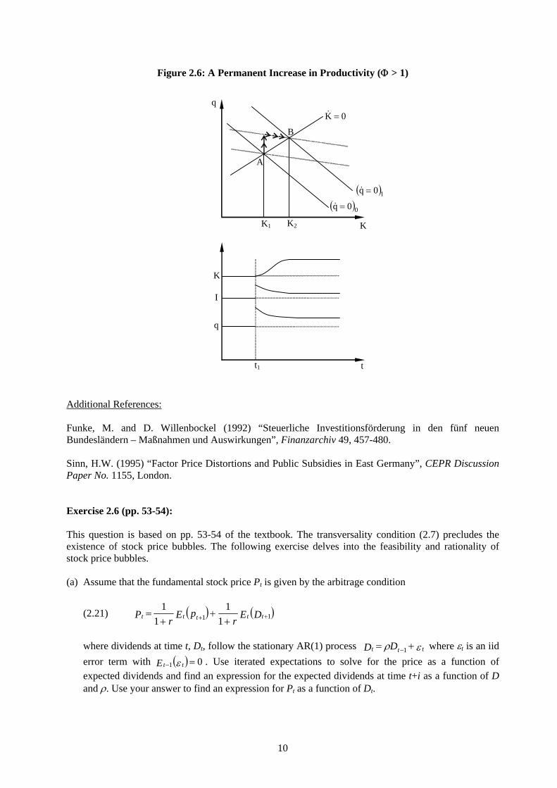
Figure 2.6: A Permanent Increase in Productivity (Φ > 1)
( )10q =&
( )00q =&
t1
q
I
K
t
0K =&
B
A
K2K1
q
K
Additional References: Funke, M. and D. Willenbockel (1992) “Steuerliche Investitionsförderung in den fünf neuen Bundesländern – Maßnahmen und Auswirkungen”, Finanzarchiv 49, 457-480. Sinn, H.W. (1995) “Factor Price Distortions and Public Subsidies in East Germany”, CEPR Discussion Paper No. 1155, London. Exercise 2.6 (pp. 53-54): This question is based on pp. 53-54 of the textbook. The transversality condition (2.7) precludes the existence of stock price bubbles. The following exercise delves into the feasibility and rationality of stock price bubbles. (a) Assume that the fundamental stock price Pt is given by the arbitrage condition
(2.21) ( ) ( )DErpErP ttttt 11 1
11
1++ +
++
=
where dividends at time t, Dt, follow the stationary AR(1) process ερ ttt DD += −1 where εt is an iid error term with . Use iterated expectations to solve for the price as a function of expected dividends and find an expression for the expected dividends at time t+i as a function of D and ρ. Use your answer to find an expression for P
( ) 01 =− ε ttE
t as a function of Dt.
10
(b) Contrary to (2.21) assume that the stock price contains a (deterministic) bubble component Bt where and B( ) BrB t
t 01+= B0>0. Prove that the price BPP ttt += ~ , where Pt~ is the fundamental share price,
is also a solution to (2.21). (c) Why are economic agents willing to pay the inflated price BPP ttt += ~ ? Solution: (a) We start by using iterated expectations to obtain
(2.22)
( ) ( )
( ) ( ) ( )
( ) ( ) ( )DErDErpErP
DErDErpErErP
DErpErP
ttttttt
tttttttt
ttttt
2
2
12
2
12121
11
11
11
11
11
11
11
11
11
11
+++
+++++
++
⎟⎠⎞
⎜⎝⎛+
++
+⎟⎠⎞
⎜⎝⎛+
=
⇔+
+⎥⎦⎤
⎢⎣⎡
++
++=
⇔+
++
=
Taking T → ∞ and assuming ( ) 01
1lim =⎟
⎠⎞
⎜⎝⎛+ +
∞→pEr Ttt
T
T, we obtain
(2.23) ( )∑ ⎟⎠⎞
⎜⎝⎛+
=∞
=+
1 11
iitt
i
t DErP .
Dividends are determined by ερ ttt DD += −1 . Therefore
(2.24)
( ) ( )( ) ( )[ ]( ) ( )[ ]
( ) .
22
1
1
1
DDE
DEDE
DEEDEDEDE
DD
ti
itt
ittitt
itttitt
ittitt
ititit
ρ
ρ
ρρρ
ερ
=
⇔=
⇔=⇔=
⇔+=
+
−++
−++
−++
+−++
M
Inserting the last equation into (2.23) yields
(2.25) ∑ ⎟⎠⎞
⎜⎝⎛+
=∞
=1 1it
i
t DrPρ .
(b) Plugging BPP ttt += ~ into (2.21) yields
(2.26) ( ) ( )
( ) ( ) ( )DErBErPErBP
DErBPErBP
tttttttt
ttttttt
111
111
11
11~
11~
11~
11~
+++
+++
++
++
+=+
⇔+
+++
=+
Since , equation (2.26) reduces to ( ) ( )BrBE ttt +=+ 11
11

(2.27) ( ) ( )DErPErP ttttt 11 11~
11~
++ ++
+=
which is identical to (2.21). Thus, we have successfully shown that the arbitrage condition holds even in the presence of a bubble. Moreover, we could even derive this result without recourse to the
condition ( ) 01
1lim =⎟
⎠⎞
⎜⎝⎛+ +
∞→pEr Ttt
T
T.
(c) Economic agents are willing to pay the higher price because they correctly anticipate that the price
will continue to rise because of the (deterministic) bubble component. The rising price yields capital gains that exactly offset the lower dividend-to-price ratio.
Exercise 2.7 (p. 68): Hartman-Abel Effect When a firm is able to adapt optimally to a changing business environment without facing adjustment costs, uncertainty may increase the value of an investment project and therefore provides an entrepreneurial opportunity. (a) Explain the principle of the so-called Hartman-Abel effect for a firm facing output price uncertainty
in a perfectly competitive market. Demonstrate the effect in graphical form. (b) Generalise the result for the case of imperfect competition. Solution: (a) We first consider a firm facing output price uncertainty under perfect competition. The mean price is P1. Now let us assume uncertainty: Let the price with a probability of 50 percent take on a value of P3 for this and all subsequent periods. Otherwise a value of P2 is assumed. The expected price thus remains at P1 (mean-preserving spread). We can now compare the expected profits under certainty versus uncertainty.
Figure 2.7: Profits under Perfect Competition and Price Uncertainty
P2
P1
P3
B
C
A
MC
Q
If prices are unexpectedly low, at P2, then profits lost are P1P2CB. If prices are unexpectedly high, at P3, then the extra profits gained would be P1P3AB. Evidently, the profits gained in good times exceed the profits lost in bad times, i.e. P1P3AB > P1P2CB. The reason is that flexible prices allow firms to exploit
12

“windfall profits” when prices are high but also to match the demand situation and cut production back when prices are low. In such a situation, uncertainty adds value to the project and one would expect that uncertainty has a positive impact upon investment. (b) Figure 2.8 below displays what happens under imperfect competition. Under price certainty, a monopoly producer will produce quantity Q1 to be sold at P1, i.e. at point (1) where marginal revenue equals marginal costs.
Figure 2.8: Profits under Imperfect Competition and Price Uncertainty
D
Q3 Q1 Q2
P2
P1
P3 A
B
MC
C
Q
D
MR
(1)
(2)
(3)
E(p)=P1
Now suppose we have a linear demand curve P = α - βQ + ε. Assuming that all other demand factors remain constant, price uncertainty will make the marginal revenue curve shift to positions such as (2) or (3). Consequently, the profit maximising monopolist would produce Q2 to be sold at P2, or Q3 at price P3, instead. At high prices P3, the profits gained would be given by area A less B. For low prices P2, the profits gained would be area C less D. As a result, the impact of uncertainty under imperfect competition is ambiguous. It depends upon the elasticity of demand. The larger the elasticity of demand and therefore the flatter the demand curve, the more the horizontal components, i.e. A and C, will dominate. In that case, expected profits will probably rise with the degree of output price uncertainty. On the contrary, the smaller the elasticity, the steeper the demand and marginal revenue curves, and the more the vertical profit components B and D will dominate. In that case expected profits will tend to fall with uncertainty. Exercise 2.8 (pp. 68-71): Hayashi (1982) has shown that if (i) the production function and the adjustment cost function are homogeneous of degree one (constant returns to scale), (ii) the stock market is efficient, and (iii) the capital goods are all homogeneous, then marginal q is equivalent to Tobin’s average q. As opposed to the homogeneity-requirement (iii), discuss the relationship between marginal q and average q for the case of heterogeneous capital goods, i.e assume that capital goods of different vintages have different technological attributes. By way of an example, discuss the impact of a sharp and persistent oil price shock upon average and marginal q. Solution: A sharp and persistent oil price shock makes energy-intensive capital goods obsolete. Therefore, the stock market value of energy-intensive firms drops and so does (observable) average q. On the other
13

hand, the marginal profit derived from installing new energy-efficient capital goods and therefore marginal q rises. If this is the case, then oil-shocks may shift average and marginal values of q in opposite directions. This is an example showing that the empirical implementation of the q-theory may be quite difficult and intricate. Exercise 2.9 [Blanchard and Fisher (1989), Problem 6, p. 310]: Consider a firm with a Cobb-Douglas production function , depreciation rate δ and quadratic adjustment costs bI . The dynamics of the capital stock is determined by
NAKY tttαα −= 1
t2 ( ) IKK ttt +−= δ1 .
The price of capital relative to the output price is normalised to one. The firm operates in competitive output and factor markets. Future wages (wt) are the only source of uncertainty. The owners of the firm have a discount rate θ. (a) Assuming that the firm chooses employment freely in each period, solve for profit maximising
employment at time t given Kt and wt. (b) Show that the optimal capital stock and optimal investment depend on current and future
expectations of wt. (c) Assume that wt follows a Markov process, i.e. wt can take of of two values w1 and w2. The (constant)
transition probabilities are given by ( ) pwwww tt ===+ 111 |prob and ( ) qwwww tt ===+ 221 |prob , respectively. Derive and explain the optimal investment process.
Solution: (a) The optimisation problem can be written as (2.28) ( ) bIwNrKKNKY ttttttt
2,max −−−−≡Π δ The first-order condition takes the form
(2.29)
( )
( )
( )
( )[ ] .1
1
01
0
11 wKAN
NKAw
wNKA
wN
YN
ttt
t
t
tt
t
t
tt
tt
αα
α
α
α
α
α
−−=⇔
⎟⎟⎠
⎞⎜⎜⎝
⎛−=⇔
=−⎟⎟⎠
⎞⎜⎜⎝
⎛−⇔
=−∂
⋅∂=∂
Π∂
Employment is increasing (decreasing) in Kt (wt). (b) Assuming risk-neutral behaviour, the net present value of future profits can be written as
(2.30) ( ) ⎥⎦⎤
⎢⎣⎡∑ Π+=∞
=+
−
0|1
iit
it tEV θ
Following Blanchard and Fisher (1989, p. 299) the quadratic cost function is given by
(2.31) ( ) Ib
KaYC tt tt22
221
⎟⎠⎞
⎜⎝⎛+−⎟
⎠⎞
⎜⎝⎛= .
14
The first term reflects the cost of producing Yt, given that the firm has capital Kt. The second term reflects quadratic costs of adjustments. Finally, the capital accumulation constraint is given by (2.32) ( ) IKK ttt +−= −11 δ . Firms are assumed to maximise the present discounted value of profits after subtracting costs of investment. Formally, the firm’s goal of maximising the net present value of profits is analogous to a minimisation of costs:
(2.33) ( ) ( ) ( )( )⎥⎦
⎤⎢⎣
⎡−+−−⎟
⎠⎞
⎜⎝⎛+−⎟
⎠⎞
⎜⎝⎛
∑ + −
∞
=
− KIKqIb
KaYE ttttti
it tt 1
22
01
221
1min δθ
where qt is the shadow price of capital. The simple recipe for the solution is to take the derivatives with respect to It and Kt which yield the following first-order conditions:
(2.34) bq
I tt =
and
(2.35) [ ] ( )KaYtqEq ttttt −++−
= + |11
1θδ .
Equation (2.34) implies that investment depends upon Tobin’s marginal q. The forward-iteration in (2.35) implies that Tobin’s q is the net present value of expected future profits. Repeated substitution leads to
(2.36)
( ) ( )
( ) ( )
( ) ( ) ( )
( ) ( ) ( )
( )KaYE
KaYKaYEKaYEqE
KaYKaYEKaYqEE
KaYKaYEqE
KaYKaYqEEq
ititi
it
i
tttttttttt
tttttttttt
ttttttt
tttttttt
++
∞
=−+
+++++++
+++++++
++++
++++
−∑ ⎟⎠⎞
⎜⎝⎛+−
=
−+−+−
+−⎟⎠⎞
⎜⎝⎛+−
+⎟⎠⎞
⎜⎝⎛+−
=
−+−+−
+⎥⎦⎤
⎢⎣⎡ −++−
⎟⎠⎞
⎜⎝⎛+−
=
−+−+−
+⎟⎠⎞
⎜⎝⎛+−
=
−+⎥⎦⎤
⎢⎣⎡ −++−
+−
=
11
11221
2
32
3
1122321
2
1121
2
1121
11
11
11
11
11
11
11
11
11
11
11
θδ
θδ
θδ
θδ
θδ
θδ
θδ
θδ
θδ
θδ
θδ
M
It must be pointed out that qt depends upon the expected future capital stock which in turn depends upon investment expenditures and therefore Tobin’s q. The two first-order conditions (2.34) and (2.35) can be written in the form
15
(2.37)
( )
( ) ( )[ ] ( )
( ) ( ) ( )
( ) ( )
( )( )( ) ( ) ( ) ( )
( )
( ) ( )( )
( )( )( ) ( )
.1
111
111
1111
111
1111
111
111
111
11111
111
11
11
11
2
2
11
11
1
δδ
θδθθ
δθθδ
δθ
θδδ
θδ
θδ
θδδ
δθδδ
θδ
−+−
++−+
+++=⇔
−+
=+−⎥⎦
⎤⎢⎣
⎡−+
−++
+−⇔
=+−
−−−⎥⎥⎦
⎤
⎢⎢⎣
⎡+
+−
+⇔
−++−
−+−
=−−⇔
−+−−+−
=−−⇒
−++−
=
−+
−+
+−
+−
+−
+
bb
Yba
KKEK
Yba
KKbb
KE
Yba
KEKKb
KaYbKKEKK
KaYbKKEKK
KaYbIEI
tttt
t
ttttt
ttttt
ttttttt
ttttttt
ttttt
Thus, the current capital stock has a forward-looking component, but it also has a backward-looking component. When the adjustment costs are more convex, i.e. b is increasing, then λ is increasing. The underlying reason for this persistence is the strictly convex adjustment costs, making it profitable to smooth investment over time. Using the method of factorisation as a toolkit, we can solve the difference equation with rational expectations (for a more detailed presentation, see Blanchard and Fisher (1989), pp. 264-266):
(2.38) ( )
( ) [ ] ,11
11
1
01
01
YNAKEba
K
YEba
KK
itititti
i
t
itti
i
tt
+−++
∞
=−
+
∞
=−
∑ ⎟⎠⎞
⎜⎝⎛+⎟⎟
⎠
⎞⎜⎜⎝
⎛−
+=
∑ ⎟⎠⎞
⎜⎝⎛+⎟⎟
⎠
⎞⎜⎜⎝
⎛−
+=
αα
θλ
δλ
λ
θλ
δλ
λ
where 0 < λ < 1 is the smaller of the root of the quadratic equation
(2.39) ( )( )( ) ( ) ( ) 0111
112 =++⎥⎦
⎤⎢⎣
⎡−+
+++
− θλδθθ
λb
b .
Using the definition of labour demand in (a), we finally obtain
(2.40) ( )( )( )[ ] [ ]wKEA
ba
KK ititti
i
ttαααα
θλ
αδ
λλ )1(
0
11 1
11
−−++
∞
=
−− ∑ ⎟
⎠⎞
⎜⎝⎛+
−⎟⎟⎠
⎞⎜⎜⎝
⎛−
+= .
According to (2.40), the optimal capital stock depends on current and future expectations of wt. In a similar vein, we obtain from (2.37) the forward-looking investment equation
16

(2.41)
( ) ( )
( ) ( )( )
( ) [ ] ( ) [ ]( )( ) .111111
11111
1111
1
)1()1(11
1
)1()1(11
11
1∑⎥⎥⎦
⎤
⎢⎢⎣
⎡−−⎟
⎠⎞
⎜⎝⎛+−
+−=
∑⎥⎥⎦
⎤
⎢⎢⎣
⎡−−⎟
⎠⎞
⎜⎝⎛+−
+−=
−∑ ⎟⎠⎞
⎜⎝⎛+−
+−=
∞
=
−−−+−+
∞
=+
−−++
−−+
++−+
∞
=
+−+i
itit
i
tt
iitititit
i
tt
itititi
i
ttt
wEaAKEbKaYb
KwKaAEbKaYb
KaYEbKaYbI
ititααααα
ααααα
αθδ
αθδ
θδ
According to (…), investment in the rational expectations model has a forward-looking component, which is a geometric discounted sum, but it also has a contemporaneous component, whereby it depends upon the current situation. (c) Without loss of generality we assume that w1 < w2. It is convenient to define the conditional expectation (2.42)
( ) ( ) ( ) ( )( ) ( ) ( ) ( )( ) ( ) ( ) ( ) ( ) ( )wwwqwwwqwwwpwwwp
wwwwwwwwwwwwwwwwwwwwwwwwwwwwwE
itititit
itititititit
itititititit
221121211111
221212121211
211112111111it1-it
probprob1prob1probprob|probprob|prob
prob|probprob|prob
=+=−+=−+=====+===+
===+====
−+−+−+−+
−+−++−+−++
−+−++−+−++++
The next step is to insert (2.42) into the forward-looking investment equation (2.41). We get (2.43)
( )
[ ] ( ) ( ) ( ) ( )( )( ) ( ) ( )( ) .1
probprob1prob1prob
1111
1
1
)1()1(1
122111
12111∑⎥⎥
⎦
⎤
⎢⎢
⎣
⎡
⎟⎟
⎠
⎞
⎜⎜
⎝
⎛−⎟⎟
⎠
⎞⎜⎜⎝
⎛=+=−
=−+=−⎟
⎠⎞
⎜⎝⎛+−
+
−=
∞
=
−−−
+−+−+−+
−+−+i
itit
i
ttt
wwwqwwpwwwqwwp
aAKEb
KaYbI
itit
ititαα
ααα αθδ
Note that a larger q implies a higher probability of a wage increase in the future, i.e.
(2.44) ( )( ) .0prob 12211 >−==
∂∂
−++−+ wwww
qwE
ititit
The evaluation of (2.44) indicates that this leads to lower investment expenditures. On the contrary, a higher p leads to a higher probability of decreasing future wages, i.e.
(2.45) ( )( ) .0prob 21111 <−==
∂∂
−++−+ wwww
pwE
ititit
It is immediately verified that this leads to higher investment expenditures. Additional Reference:
Blanchard, O.J. and S. Fisher (1989) Lectures on Macroeconomics, Cambridge (MIT Press).
17

Exercise 2.10 (pp. 82-83 on the Wiener process): Explain the meanings of the Wiener process; show that the process has no memory of the past and any shocks are permanent; show that the process is a diffusion process of time. Solution: The Wiener process is the simplest diffusion process (stochastic process) describing what are known as Brownian motions in physics. Most stochastic processes may be described in terms of a standard Wiener process. The Wiener process is a continuous-time stochastic process named in honour of Norbert Wiener. It is often also called a Brownian motion, after Robert Brown. It is one of the best known Lévy processes and occurs frequently in pure and applied mathematics, economics and physics. The Wiener process plays an important role both in pure and applied mathematics. In pure mathematics, the Wiener process gave rise to the study of continuous time martingales. It is a key process in terms of which more complicated stochastic processes can be described. As such, it plays a vital role in stochastic calculus and in diffusion processes. It is also prominent in the mathematical theory of finance, in particular the Black-Scholes option pricing model. In physics it is used to study Brownian motion, the diffusion of minute particles suspended in fluid. Definition: The standard Wiener process is a Gaussian process on a probability space with independent increments for which (2.46) , 00 =W [ ] [ ]0 0tE W E W= = , [ ]t sVar W W t s− = − for all ts ≤≤0 , where each increment is independent to each other and the path for is continuous. tW
(a) , 00 =W [ ] [ ]0 0tE W E W= = , and [ ]tVar W t= correspond to the random walk properties. In terms of a
Gaussian representation, we have ( )~ 0;tW N t . [ ] 0tE W = represents the property that the expected movements from W is zero and each step for W follows a normal distribution increment of
. Though the process for is continuous, there is no relationship at all between increments (a random walk). This property also relates to “lack of memory”. The past history of the movements has no impact on its future position. The future movement of the process only depends on its present position but it does not depend on how the process got there. This implies that “independent increments” satisfies the Markov property.
(~ 0;t sW W N t s− )−
)−
tW
(b) Gaussian process: . With zero mean (no drift), the motion (movement) has no more tendency towards one direction than the opposite direction. The central limit theorem makes it reasonable to assume that the increments are normally distributed. The corresponding normal distribution function for the increment
(~ 0;t sW W N t s−
( )~ 0;t sW W N t s− − , 0 s t≤ < , has the following transition density
(2.47) ( )( )
( )( )
2
21,2
y xt s
t s s tp W W W x W y et sπ
−−
−− = = =−
,
Therefore, we have
(2.48) [ ] 0t sE W W− = , ( )2t sE W W t s⎡ ⎤− = −⎣ ⎦ ,
18

and with the property , we have 0 0W = (2.49) [ ] 0tE W = , 2
tE W t⎡ ⎤ =⎣ ⎦ .
(c) The fact , along with the “no drift” property, implies that the variance grows
with the length of the interval and the process tends to wander away from its original position and no force pulls it back to the original position – any shocks are permanent. The covariance for 0
( )2t sE W W t s⎡ ⎤− =⎣ ⎦ −
s t≤ < is
(2.50)
[ ] [ ] [ ][ ] [ ]
( )[ ] [ ] ( )
cov , cov , cov ,
var cov ,
min , .
s t s t s s t
s s t s
s t s
s t s
W W W W W W W W
W W W W
s E W W W
s E W E W W s s t
= = +
= + −
⎡ ⎤= + −⎣ ⎦= + − = =
s−
Some textbooks might add the following property: For each outcome is continuous in t, . It is reasonable that a Wiener process is a continuous function of t. Proofs of continuous sample functions are known but are too complex to warrant inclusion in this Study Guide.
tW 0t ≥, tW t T∈
A Wiener process is a normalised “random walk” process and can be written as follows (2.51) t tdW dtε= , where tε is a normally distributed Gaussian process with mean zero and a standard deviation of unity
and thus ( )~ 0,1t Nε (2.52) ( )~ 0;tdW N dt . The random variable tε is serially uncorrelated. Thus values of W for any two different time intervals are independent. Exercise 2.11 (p. 16 and p. 83; random walk): To take the analysis a bit further, show the properties of the discrete-time random walk and its relationship to the Wiener process. Solutions: The simplest random walk form of a time series is denoted by the following equation: (2.53) 1t t ty y u−= + , t =1…T, where the errors are independently and identically normally distributed with mean 0 and finite
variance tu
2uσ and also called a white noise process with ( )2~ 0;t uu N σ and for ( )cov , 0s tu u = s t≠ .
It is easy to show that
19

(2.54) 1 2 1 0 1 01
...t
t t t t t t ty y u y u u y u u y uττ
− − −=
= + = + + = + + + = +∑ .
Equation (2.54) shows that shocks persist and ty doesn’t return to the initial point. In line with this, autoregressive models in econometrics contain a unit root if the coefficient |b| = 1 in
ttt byay ε++= −1 , where is the variable of interest at time t, b is the slope coefficient, and ty tε is the error component. If a unit root is present, the time series is said to have a stochastic trend, be nonstationary, or being integrated at order one or I(1). On the contrary, for |b| < 1, the time series is stationary, or I(0). With the assumption of independence of , the mean and variance of tu ty are denoted by
(2.55) [ ] 0 01
t
tE y E y u yττ =
⎡ ⎤= + =⎢ ⎥
⎣ ⎦∑ ,
(2.56) [ ] 2var t uy tσ= . This implies that ty has the following distribution: (2.57) ( )2
0~ ;t uy N y tσ .
The standard deviation grows with the square root of time. Equation (2.57) also implies that (2.58) ( )2~ 0;t uy N tσΔ Δ .
Equation (2.53) can be written in terms of “increments” and a standard Gaussian white noise: (2.59) 1t t t uy y y tσ ξ+Δ = − = , where tξ is Gaussian white noise with ( )~ 0;1t Nξ and ( )cov , 0s tξ ξ = , ). Any “increments”
are with zero mean and independent with each others. The process
s t≠
ty tends to wander around and there are no more tendencies in one direction than in the opposite direction. The future movement of ty only depends on its present value - it does not depend on how it got there. The past history, say 0y , has no impact on its future position 1ty + . If we rewrite (2.59) into a continuous-time diffusion process, we then have
(2.60) t ud ydt tσ ξ= .
The question now becomes how to transform a standard Gaussian white noise tξ into a continuous-time
limit of the discrete time process. We know from (2.51) that the Wiener process follows t tdW dtε= , where tε is a normally distributed Gaussian process with mean zero and a standard deviation of unity
and thus and the random variable (~ 0,1t Nε ) )(~ 0;tdW N dt tε is serially uncorrelated.
20

From equation (2.58), we have (2.61) ( ) ( )2 2~ 0; ~ 0;t u ty N t dy N dtσ σΔ Δ ⇒ u .
Therefore, equations (2.60), (2.52) and (2.61 together imply that
(2.62) tt
dWdt
ξ = .
Symbolically, it can be written as tdt dWtξ = , which is known as Langerm’s equation. Thus, the random walk process of equation (2.62) becomes (2.63) t udy dWtσ= . Note that equation (2.63) is problematic since the sample paths of a Wiener process cannot be differentiated. Exercise 2.12 (pp. 84-85 on Ito’s process and lemma): (a) Derive the mean and variance of the Ito’s process ( ) ( ), ,t t tdX a t X dt b t X dW= + t . (b) Show why we cannot ignore the second derivatives terms in Ito’s Lemma. Explain in terms of
Taylor’s expansions. Solutions: (a) An Ito process X implies that the drift term and diffusion term are both a function of time and X, (2.64) ( ) ( ), ,t t tdX a t X dt b t X dW= + t or (2.65) ( ) ( ), ,dX a t X dt b t X dW= + . Since [ ] 0tE dW = , we have (2.66) [ ] ( ),t tE dX a X t dt= ,
(2.67) [ ]var tdW dt= . We can therefore calculate
(2.68)
[ ] [ ] ( ) ( )[ ] ( ) ( )
( ) [ ] ( )
2 22 2
22 2 2 2 2
22 2 2 2
var
2
var , .
t t t
t
dX E dX E dX E adt bdW a dt
a dt abdtE dW b E dW a dt
b E dW b dW b dt b X t dt
⎡ ⎤⎡ ⎤= − = + −⎣ ⎦ ⎣ ⎦⎡ ⎤= + + −⎣ ⎦
⎡ ⎤= = = =⎣ ⎦
2
21

(b) Ito’s Lemma: Consider a continuous and differentiable function F of an Ito process: ( ), tF F t X≡ ,
where . If we disturb the system a bit so that there is a small change in the Ito process, the function F can then be expanded by a Taylor series,
( ) ( ), ,t t tdX a t X dt b t X dW= + t
(2.69) ( ) ( )
( )2
, ,1 higher order terms,2t X XX
F F t t X X F t X
F t F X F X
Δ = + Δ + Δ −
= Δ + Δ + Δ +
where tF F t≡ ∂ ∂ , XF F X≡ ∂ ∂ , and 2
XX2F F X≡ ∂ ∂ . Note that we cannot ignore the second order
term when taking limits since
(2.70) . ( ) ( ) ( ) ( )2 2 2 22 2 22E X E a t ab t W b W b E W b⎡ ⎤ ⎡ ⎤ ⎡ ⎤Δ = Δ + Δ Δ + Δ ≅ Δ =⎣ ⎦ ⎣ ⎦ ⎣ ⎦2 tΔ
On the other hand we can ignore the terms of order ( )3 2dt from [ ]E t WΔ Δ and the term ( when
compared to . Taking limits
)2tΔ
( )2E W⎡ ⎤Δ =⎣ ⎦ tΔ tt dΔ → of (2.69) gives
(2.71) 212t X XXdF F dt F dX F dX= + + .
Substituting the Ito process (2.64) into the above equations gives
(2.72) ( ) 212t X XXdF F dt F adt bdW F b dt= + + + .
After collecting terms, we then have Ito’s lemma
(2.73) ( ) ( ) ( )21, , ,2t X XXdF F a t X F b t X F dt b t X F dW⎛ ⎞= + + +⎜ ⎟
⎝ ⎠X
Note that we do not derive Ito’s Lemma here. We would need the stochastic integrals and several pages to present a rigorous proof of Ito’s lemma. Those who are interested can refer to formal textbooks. See, for example, Øksendal (2000), Sections 4.1 and 4.2; Kloeden and Platen (1992), Chapter 3, or Brzezniak and Zastawniak (1998), Chapter 7. The book by Brzezniak and Zastawniak (1998) is probably a good introduction in stochastic processes if your maths/stats background is not so strong. References: Brzezniak, Z. and T. Zastawniak (1998) Basic Stochastic Processes: A Course Through Exercises, Berlin (Springer-Verlag). Kloeden, P. E., and E. Platen (1992) Numerical Solution of Stochastic Differential Equations, Berlin (Springer-Verlag). Øksendal, Bernt (2000) Stochastic Differential Equations. An Introduction with Applications, 5th edition, Berlin (Springer-Verlag).
22

Exercise 2.13: (pages 84-85 on Ito’s integrals): Note: Stochastic calculus is difficult and only covered in a rudimentary fashion in this short guide. Please consult formal textbooks for this topic. Here we only discuss the basic properties. Note that since it is not discussed in a rigorous way, the results here are only serve as intuitive observations, and provide the background for simple numerical simulations. Show
(a) the properties of the integral ( )0
t
sb s dW∫ ;
(b) the properties of the integral 0
t
ssdW∫ .
(c) the properties of the integral 0
t
s sW dW∫
Solutions: A stochastic process (2.74) ( ) ( ), ,t t tdX a t X dt b t X dW= + t
s
can be interpreted mathematically as a stochastic integral equation
(2.75) ( ) ( )0
0 0
, ,t t
t t s st tX X a s X ds b s X dW= + +∫ ∫ ,
where is a deterministic Riemann-Stieltjis integral and is an Ito
stochastic integral that cannot be a Riemann-Stieltjis. Note that for a Riemann-Stieltjis integral,
( )0
,t
tta s X ds∫ ( )
0
,t
ttb s X dW∫ t
(2.76) ( ) ( ) ( ) ( ) ( )1
100
limNT
j j jN jf s dR s f R t R tτ
−
+→∞=
⎡ ⎤= −⎣ ⎦∑∫ ,
where jτ is arbitrary and , which is very robust. However, for an Ito stochastic integral, 1,j j jt tτ +⎡∈ ⎣ ⎤⎦
t
(2.77) ( ) ( ) ( ) ( ) ( )1
1
00
, lim ,j j
NT
s j tN jf s dW f t W Wω ω ω ω
+
−
→∞=
ω⎡ ⎤= −⎣ ⎦∑∫ ,
where ω is the random varialble. ( ),jf t ω is always computed at the beginning of each subinterval. For
the time step and its corresponding 1n nt +Δ = − nt nt1nn tW W W+
Δ = − , the Ito stochastic process becomes (2.78) ( ) ( )1
, , , 0, 1, 2,...n n n nt t n t n n t nX X a t X b t X W n+= + Δ + Δ = ,
which is the stochastic Euler scheme. The Ito stochastic integral becomes
(2.79) ( ) ( )1 00 0
, , , 0, 1, 2,...n n n
n n
t t n t n n t nn n
X X a t X b t X W n+
= =
= + Δ + Δ =∑ ∑
23
(a) If is not a function of ( ).b tX , it is then easy to show that
(2.80) , ( ) ( ) ( ) [ ]0
0 0
0n nt
t n n nn n
E b s dW E b t W b t E W= =
⎡ ⎤⎡ ⎤ ≡ Δ = Δ⎢ ⎥⎢ ⎥⎣ ⎦ ⎣ ⎦∑ ∑∫ n =
2
)Δ
since is a Wiener process. And its variance is given by tW
(2.81) , ( ) ( ) [ ] ( ) ( )2 2
0 00 0
var varn nt t
s n n n nn n
b s dW b t W b t t b s ds= =
⎡ ⎤ ≡ Δ = Δ ≡⎢ ⎥⎣ ⎦ ∑ ∑∫ ∫
since the Wiener process is independent and normally distributed with . These properties will be used in mean-reverting processes in the next exercise.
(~ 0;tW N tΔ
(b) Let s sX sW= . Ito’s lemma gives ( )s sd sW W ds sdW= + s . Taking integrals implies that
, which is the same as the integration by parts in Leibnitzian calculus. 0 0
t t
s t ssdW tW W ds= −∫ ∫ (c) Let 2
s sX W= . Ito’s lemma gives ( )2 2s s sd W W dW ds= + . Taking integrals gives that
2
02
t
s s tW dW W t= −∫ 2 , which is not the same as in integration in Leibnitzian calculus:
2
02
t
s s tx dx x=∫ .
Exercise 2.14 (pp. 84-85 on the applications of Ito’s Lemma to different stochastic processes): To take the analysis a bit further, discuss the properties of the following stochastic processes: (a) A Brownian motion with drift: t tdX dt dWα σ= + ; (b) A geometrical Brownian motion: dX Xdt XdWα σ= + (c) An Ornstein-Uhlenbeck process: ( )t tdX X X dt dWη σ= − + t .
Solutions: (a) The standard Wiener process can be generalised to a Brownian motion with a drift: (2.82) t tdX dt dWα σ= + , where is the standard Wiener process, tW α is the drift parameter, and σ the variance parameter. This process is usually used to approximate for stationary variables, such as interest rates, inflation rates, etc. It is easy to show that (2.83) [ ]tE dX dtα= , [ ] 2var tdX dtσ= ( )2~ ;tdX N dt dtα σ ;
and intuitively we can have (2.84) ( )2
0~ ;tX N X t tα σ+ , [ ] 0tE X X tα= + .
24
Alternatively, we can use the stochastic integral:
(2.85) 0 00 0
t t
t sX X ds dW X t Wtα σ α= + + = + +∫ ∫ σ .
Therefore, the mean and variance of tX are (2.86) [ ] [ ]0 0t tE X X t E W X tα σ α= + + = + , and
(2.87)
[ ] ( ) [ ]
( ) ( ) [ ] ( )[ ]
2 20 0
2 22 20 0 0
2 2 2 2
var
2
var .
t t
t t
t t
X E X t W E X t
X t X t E W E W X t
E W W t
α σ α
α α σ σ
σ σ σ
⎡ ⎤= + + − +⎣ ⎦
⎡ ⎤= + + + + − +⎣ ⎦⎡ ⎤= = =⎣ ⎦
α
Note: If the stochastic processes are linear scalar ones, we can take the expectations [ ]tE dX and obtain
the expected solutions for tX accordingly. Thus, ( ) 0t tE dX dt X X tα α= ⇒ = + . Let . Using Ito’s lemma gives XF e=
(2.88) 212
dF Fdt FdWα σ σ⎛ ⎞= + +⎜ ⎟⎝ ⎠
,
which shows that F follows a geometrical Brownian motion. (b) A geometric Brownian motion (GBM) (occasionally, exponential Brownian motion) is a continuous-time stochastic process in which the logarithm of the randomly varying variable follows a Brownian motion, or a Wiener process. It is appropriate for the modelling of some issues in mathematical finance. It is used particularly in the field of option pricing because a variable that follows a GBM may take any value strictly greater than zero, and only the fractional changes of the random variable are significant. This is precisely the nature of a stock price, which can never take on negative values: (2.89) dX Xdt XdWα σ= + , where W is the standard Wiener process, α is the drift parameter, and σ the variance parameter. It is easy to show that (2.90) ( )E dX Xdtα= , [ ] 2 2var dX X dtσ= , ( )2 2~ ;dX N Xdt X dtα σ ,
which are difficult to discuss in terms of the distribution since X itself is involved in the Gaussian distribution notation. It is then convenient to use Ito’s lemma to have the lognormal distribution. Let
. Using Ito’s lemma, we obtain lnF = X
(2.91) 2 2 21 12 2t X XX XdF F XF X F dt XF dW dt dWα σ σ α σ σ⎛ ⎞ ⎛= + + + = − +⎜ ⎟ ⎜
⎝ ⎠ ⎝⎞⎟⎠
,
25

since 0,tF = 1XF = ,X and 21XXF X= − . ln X then follows a generalised Wiener process
(2.92) 2 21ln ~ ;2tX N tα σ σ⎛ ⎞⎛ ⎞−⎜ ⎟⎜ ⎟
⎝ ⎠⎝ ⎠t .
The Ito stochastic integral for 212tdF dt dWα σ σ⎛ ⎞= − +⎜ ⎟
⎝ ⎠ gives the following result
(2.93) 20
12t tF F t Wα σ σ⎛ ⎞= + − +⎜ ⎟
⎝ ⎠.
Substituting into the above equation yields lnF = X
(2.94) 21
2 20 0
1ln ln2
tt W
t t tX X t W X X eα σ σ
α σ σ⎛ ⎞− +⎜ ⎟⎝ ⎠⎛ ⎞= + − + ⇒ =⎜ ⎟
⎝ ⎠.
Taking expectation gives
(2.95) [ ]21
20
tt
WtE X X e E e
α σσ
⎛ ⎞−⎜ ⎟⎝ ⎠ ⎡ ⎤= ⎣ ⎦ .
The lognormal distribution shows
2 2tW tE e eσ σ⎡ ⎤ =⎣ ⎦ , where ( )~ 0;tW N t :
(2.96)
( )
( )
2 22 2 2
222 2
1 122 22 2
1 11 1 12 22 2 2
1 1 12 2 2
1 1 ,2 2
t
xx x x t tx tW x t t
x t x tt tt t2t
E e e e dx e dx et t t
e e dx e e dx et t
σ σ σσσ σ
σ σσ σ σ
π π π
π π
⎛ ⎞⎛ ⎞⎜ ⎟∞ ∞ ∞ − − + +⎜ ⎟− − ⎜ ⎟⎝ ⎠⎝ ⎠
−∞ −∞ −∞
⎛ ⎞∞ ∞− −⎜ ⎟ − −⎝ ⎠
−∞ −∞
⎡ ⎤ = = =⎣ ⎦
= = =
∫ ∫ ∫
∫ ∫
dx
since ( )2 21 1
2 21 1 1,2 2
x t yt te dx e dy
t tσ
π π
∞ ∞− − −
−∞ −∞
= =∫ ∫ where y x tσ= − . After taking a long route, we
finally have (2.97) [ ] 0
ttE X X eα= .
Note: The result [ ] 0
ttE X X eα= for dX Xdt XdWα σ= + is obvious since tX is a linear scalar
stochastic process. The result of [ ]E dX Xdtα= would give [ ] 0t
tE X X eα= . Another intuitive way to
obtain the lognormal distribution results is via Ito’s lemma. Let Wy eσ= . We have
(2.98) [ ] 2 21 12 2tE dy E ydW ydt ydtσ σ σ⎡ ⎤= + =⎢ ⎥⎣ ⎦
.
26

Thus, we have [ ] 2 2tE y eσ= for a linear scalar stochastic process of dy. Later on we will see that this convenient way doesn’t work on a geometrical mean-reverting process since it is not a linear scalar stochastic process. The variance is obtained by the following:
(2.99) [ ]2 2
21 1222 22 220 0 0var
tt
t W tWt t
t2
0X E X e E X e X e E e X eα σ σ α σ
σα α⎛ ⎞⎛ ⎞ ⎛ ⎞− + −⎜ ⎟⎜ ⎟ ⎜ ⎟⎝ ⎠⎝ ⎠ ⎝ ⎠
⎡ ⎤⎛ ⎞⎢ ⎥ ⎡ ⎤⎜ ⎟ ⎡ ⎤= − =⎣ ⎦ ⎣ ⎦⎢ ⎥⎜ ⎟⎝ ⎠⎣ ⎦
− .
By the lognormal distribution, we have
22 2tW tE e eα α⎡ ⎤ =⎣ ⎦ . Or by Ito’s lemma, we have
[ ] 22 2 2t2E dy E ydW ydt ydtα α α⎡ ⎤= + =⎣ ⎦ , where 2 tWy e α= . Since dy is linear scalar in y, we have
22 2tW tE e eα α⎡ ⎤ =⎣ ⎦ Therefore, the variance of tX is
(2.100) [ ] ( )2
2 212
2 2 2 2 2 220 0 0var 1
tt t t t
tX X e e X e X e eα σ
σ α α σ⎛ ⎞−⎜ ⎟⎝ ⎠= − = − .
The expected value of a stochastic process tX is important since with it, it is possible to compute the intertemporal discount value of tX . For example,
(2.101) [ ] 000 0 0
t t t tt t
XE X e dt E X e dt X e e dtρ ρ α ρ
ρ α∞ ∞ ∞− − −⎡ ⎤ = = =⎢ ⎥⎣ ⎦ −∫ ∫ ∫ ,
if ρ α> . (c) The mean-reverting Ornstein-Uhlenbeck process have been used, for example, by economists to model the term structure of interest rates in finance and exchange rate dynamics within target zone regimes. Those who are interested in the target zone applications could see Ball and Roma (1993), Froot and Obstfeld (1991), Krugman (1991) and Stegenborg Larsen and Sørensen (2007). The Ornstein-Uhlenbeck process is represented by (2.102) ( )t tdX X X dt dWη σ= − + t ,
where 0η ≥ is the speed of mean-reverting, σ is the variance parameter, and X is the “normal” or “target” level of X. As η approaches 0, it becomes a Brownian motion without a drift. The expected values of and tdX tX is (2.103) [ ] ( )t tE dX X X dtη= − .
Intuitively, the process of [ ]tE X could be obtained from the above equation since is linear in tdX tX : (2.104) [ ] ( )0
ttE X X X X e η−= + − .
27
Formally, the results of the above equation can be obtained via the following stochastic integral of a mean-reverting process,
(2.105) ( )0 0
tt t st sX X X X e e e dWη η ησ− −= + − + ∫ .
Note: Luckily, mathematicians have done a great job solving most of stochastic differential equations for us. For example, you can find many explicitly solvable SDEs in Chapter 4 of Kloeden and Platen (1992). We can firstly simplify the mean-reverting process by setting
t tY X X= − . Therefore, the mean-reverting process becomes t tdY Y dt dWtη σ= − + . The stochastic process is linear in . Its solutions should
have the component of tY
te η− . Let tt tY y e η−= ⇒ t
t ty Y eη= . Ito’s lemma gives . The corresponding stochastic integral is
denoted by ( )t t t t t
t t t t t tdy Y e dt e dY Y e dt e Y dt dW e dWη η η η ηη η η σ= + = + − + = tσ
s
0 00 0
t ts st sy y e dW y e dWη ησ σ= + = +∫ ∫ .
Substituting t
t ty Y eη= and t tY X X= − back into the above equation yields the solutions. Take expectation
of equation (2.105) and we have
(2.106) [ ] ( ) ( )0 00
tt t st sE X X X X e e E e dW X X X e tη η ησ− − ⎡ ⎤= + − + = + −⎢ ⎥⎣ ⎦∫ η− .
Since 0
t ssE e dWη⎡
⎢⎣∫⎤⎥⎦
=0 according to (2.80). And the variances are denoted by
(2.107) [ ] ( )( )
( ) ( )
2 20 0 0
2 2 2 2 22 2 2 2 2 2
0 0
var var var
1 1 .2 2 2
t tt t s t st s
t tt tt s s t t
sX X X X e e e dW e e dW
e ee e ds de e e
η η η η η
η ηη η η η η
σ σ
σ σ σση η η
− − −
− −− −
⎡ ⎤ ⎡ ⎤= + − + =⎢ ⎥ ⎢ ⎥⎣ ⎦⎣ ⎦
= = = − = −
∫ ∫
∫ ∫
Note that and come from the discussions in the last
section. 0
0t s
sE e dWη⎡ ⎤ =⎢ ⎥⎣ ⎦∫ 2
0 0var
t tsse dW e dsη⎡ ⎤ =⎢ ⎥⎣ ⎦∫ ∫ sη
References: Ball, C.A. and A. Roma (1993) “A Jump Diffusion Model for the European Monetary System”, Journal of International Money and Finance 12, 475-492. Froot, K.A. and M. Obstfeld (1991) “Exchange Rate Dynamics Under Stochastic Regime Shifts: A Unified Approach”, Journal of International Economics 31, pp. 203-229. Krugman, P. (1991) “Target Zones and Exchange Rate Dynamics”, Quarterly Journal of Economics 106, 669-682. Stegenborg Larsen, K. and M. Sørensen (2007) “Diffusion Models for Exchange Rates in a Target Zone”, Mathematical Finance 17, 285-306.
28
Exercise 2.15 (pp. 85 on Ito’s Lemma to different stochastic processes): (a) Explain the meaning of (2.49) in the textbook by using Bellman equation; (b) Derive (2.50) in the textbook by applying Ito’s Lemma to Bellman equation. Solutions: Subquestion (a): The continuous-time Bellman equation is widely used in the investment under uncertainty literature. Suppose that the exogenous discount rate is ρ and there is a flow payoff (profit, dividend, utility, etc), ( ),t tX uπ , where π is a function of tX – this could be a stochastic process – and
control variable . The expected present (intertemporal) value tu ( )t tV X starting at time = t is denoted by
(2.108) ( ) ( ) ( )max , tt t tu
t
V X E X u e dρ ττ τπ τ
∞− −⎧ ⎫⎡ ⎤⎪ ⎪= ⎨ ⎬⎢ ⎥
⎪ ⎪⎣ ⎦⎩ ⎭∫ .
If there is no uncertainty, then E[.] is discarded. For an investment problem, the value function denotes the value of the investment project. The discount rate ρ here represents annual required rate of the return for this investment. If investors hold this asset (investment project) over some period (say dt), this asset will yield a dividend (cash flow) rate ( ) ( ),t t t tX u V Xπ . The expected capital gain rate during this
period is ( ) ( )1 t t t tV E dV X d⎡ ⎤× ⎣ ⎦ t . In equilibrium, the required rate of return for this investment, ρ ,
should be equal to the sum of the dividend yield ( ) ( ),t t t tX u V Xπ and the expected capital gain rate
( ) ( )1 t t t tV E dV X d⎡ ⎤× ⎣ ⎦ t in a no arbitrage condition. If the required return ρ is greater than
dividend/capital gains ( ) ( ),t t t tX u V Xπ + ( ) ( )1 t t t tV E dV X dt⎡ ⎤× ⎣ ⎦ , then the value of this firm is too
high. The value of the firm should fall since no one wants to hold this investment (buy this firm’s shares). If the required rate of returns is less than dividend/capital gains, then the value of this firm is valued too low. The value of the firm should be raised since every rational investor wants to undertake this investment (buy this firm’s shares). In equilibrium, the following equation should hold:
(2.109) ( ) ( )( )
max , t t tt t t tu
E dV XV X X u
dtρ π
⎧ ⎫⎡ ⎤⎪ ⎪⎣ ⎦= +⎨ ⎬⎪ ⎪⎩ ⎭
,
which the continuous-time Bellman equation.
Digression: As an aside, note that the Bellman equation can be obtained from the simple definition of the value function. The value function can be written as follows: (2.110)
( ) ( ) ( )
( ) ( ) ( ) ( )
max ,
max , , .
tt t tu
t
t tt t
t tut t t
V X E X u e d
E X u e d E X u e d
ρ ττ τ
ρ τ ρ ττ τ τ τ
π τ
π τ π τ
∞− −
+Δ ∞− − − −
+Δ
⎧ ⎫⎡ ⎤⎪ ⎪= ⎨ ⎬⎢ ⎥⎪ ⎪⎣ ⎦⎩ ⎭⎧ ⎫⎡ ⎤ ⎡ ⎤⎪ ⎪= +⎨ ⎬⎢ ⎥ ⎢ ⎥⎪ ⎪⎣ ⎦ ⎣ ⎦⎩ ⎭
∫
∫ ∫
The term ( ) ( ),t t t
tX u dρ τ
τ τπ τ+Δ − −
∫ can be proxied by
29

(2.111) ( ) ( ) ( ) ( ), ,t t t tt t
t t t tt tX u e d X u e d X u tρ τ ρ
τ τπ τ π τ π+Δ +Δ− − − Δ ,≅ ≅ Δ∫ ∫ ,
if approaches to zero. The intuition is very simple. With tΔ 0tΔ → , the discount factor should approach 1 and the area (integral) can be approximated by ( ),t tX u tπ ×Δ . The second term of the right-hand side of equation (2.110) can be transformed into the following:
(2.112) ( ) ( ) ( ) ( )( )
( )
, ,
.
t tt tt t
t t t t
tt t t t t
E X u e d E e X u e d
e E V X
ρ τρ τ ρτ τ τ τ
ρ
π τ π∞ ∞
− − +Δ− − − Δ
+Δ +Δ
− Δ+Δ +Δ
⎡ ⎤ ⎡=⎢ ⎥ ⎢
⎣ ⎦ ⎣⎡ ⎤= ⎣ ⎦
∫ ∫ τ⎤⎥⎦
Substituting equations (2.111) and (2.112) back to (2.110) gives the well-known continuous-time Bellman’s principle of dynamic programming: (2.113) ( ) ( ) ( ){ }max , t
t t t t t t t t tuV X X u t e E V Xρπ − Δ
+Δ +Δ⎡ ⎤= Δ + ⎣ ⎦ .
Using the fact that 1te ρ tρ− Δ ≅ − Δ by power-series approximation and rearranging equation (2.113) yields (2.114) ( ) ( ) ( ) ( ) ( ){ }max , 1t t t t t t t t t t tu
tV X X u t t E V X V Xρ π ρ +Δ +Δ⎡ ⎤Δ = Δ + − Δ −⎣ ⎦ .
Divide by and take limits such that tΔ
0lim
tt dt
Δ →Δ = . We obtain
(2.115) ( ) ( )( )
max , t t tt t t tu
E dV XV X X u
dtρ π
⎧ ⎫⎡ ⎤⎪ ⎪⎣ ⎦= +⎨ ⎬⎪ ⎪⎩ ⎭
,
where is the Hamilton-Jacobi-Bellman (or abbreviated as the Bellman) equation. Note that the above proof holds if the intertemporal value is integrated from t to T, not to infinity.
The shadow price capital, the value function of marginal capital, is represented by (2.48) in the
textbook: ( ) ( )( )'T r t
t t tE F K Z e dδ τ
τ τλ τ− + −⎡= ⎢⎣∫⎤⎥⎦
. Therefore, the corresponding Bellman equation is
denoted by
(2.116) ( ) ( ) [ ]' t tt t t
E dr F K Z
dtλ
δ λ+ = + .
The left-hand side denotes the required effective rate of return for the marginal contribution of capital; the right-hand side represents the sum of current marginal revenue and the capital gain at t. In equilibrium the equation must hold. The meaning of equation (2.49) in the textbook is then obvious since it is just a variant of (2.116). Subquestion (b): If tX follows a general Ito process discussed in (2.74):
( ) ( ), ,t t t tdX a t X dt b t X dW= + , by Ito’s Lemma, we have the following relation:
30
(2.117) ( )
( ) ( )21, ,2
t t tt X
E dV XV a t X V b t X V
dt⎡ ⎤⎣ ⎦ = + + XX .
Substituting into the Bellman equation (2.109) gives
(2.118) ( ) ( ) ( ) ( )21max , , ,2t t t t t t X t XXu
V X X u V a t X V b t X Vρ π⎧ ⎫= + + +⎨ ⎬⎩ ⎭
.
The Bellman equation is often unsolvable since it is hard to obtain the solutions to the partial differential equation after optimisation. Therefore, most of the time it is assumed the value function starts from
and the drift and risk parameters are time-invariant, such as 0t = (2.119) ( ) ( )t t tdX a X dt b X dW= + t . The value function and equation (2.118) then becomes
(2.220) ( ) ( ) 00
max ,u
t
V X E X u e d X Xρττ τπ τ
∞−
=
⎧ ⎫⎡ ⎤⎪ ⎪= =⎨ ⎬⎢ ⎥⎪ ⎪⎣ ⎦⎩ ⎭
∫ ,
Subject to ( ) ( )dX a X ds b X dWτ τ τ τ . The Bellman equation after applying Ito’s lemma becomes = +
(2.221) ( ) ( ) ( ) ( )21max ,2X Xu
V X X u a X V b X Vρ π X⎧ ⎫= + +⎨ ⎬⎩ ⎭
.
For the textbook problem for (2.48) ( ) ( )( )'T r t
t t tE F K Z e dδ τ
τ τλ τ− + −⎡ ⎤= ⎢ ⎥⎣ ⎦∫ subject to the capital
depreciation process t tdK K dtδ= − and a geometrical Brownian motion t t tdZ Z dt Z dWtθ σ= + , we have
(2.222) ( ) 2 2, 1
2t t
K Z Z
E d K ZK Z Z
dtλ
Zδ λ θ λ σ λ⎡ ⎤⎣ ⎦ = − + +
by total differentiation with chain rules and Ito’s Lemma with the assumption of the value function integrating from t=0. Substituting into the Bellman equation (2.116) gives
(2.221) ( ) ( ) 2 21'2K Z Zr F K Z K Z Z Zδ λ δ λ θ λ σ+ = − + + λ .
Substituting kP qλ = into the above equation gives (2.50) in the textbook.
31
II. Software Tools Software-Exercise 2.1: A Simple Numerical Method – The Euler Scheme for the Geometrical Brownian Motion and the Ornstein-Uhlenbeck process The stochastic Euler scheme (see equation (2.78), exercise 2.10) (2.222) ( ) ( )1
, , , 0, 1, 2,...n n n nt t n t n n t nX X a t X b t X W n+= + Δ + Δ =
is the standard numerical procedure consistent with Ito Integrals. Assume that the time partition is denoted by , where . The step size is denoted by 0 1, , ..., Nt t t 0t t T≤ ≤ 1n nt + ntΔ = − . Usually we would consider a uniform time discrete approximation and set the initial time as . This means that 0 0t =
(2.223) 1n n nTt tN+Δ ≡ Δ = − = ,
and (2.224) ,
1n nn tW W W+
Δ = − t
N − for . Therefore, the Euler scheme can be written as 0, 1, ..., 1n = (2.225) ( ) ( )1 , , , 0, 1, 2,...n n n n n n nX X a t X b t X W n+ = + Δ + Δ = . By the definition of the Wiener process, the random variables nWΔ are independent normally distributed with means and variances (2.226) ( )~ 0;nW NΔ Δ , [ ] 0nE WΔ = and [ ]var nWΔ = Δ . For a given sample path ( )tW ω and initial value of ( )0X ω , we can obtain the approximate sample
path nX , once the noise sample path approximate, , is realised. It is easier to proxy the independent
noise increment nW
( )~ 0;nW NΔ Δ by a normal standard Gaussian ( )0;1N . We can write (2.227) n nW εΔ = Δ , [ ] 0nE WΔ = and [ ]var nWΔ = Δ , where and (~ 0;1n Nε ) nε is serially uncorrelated.
32

The sample path of nX
0t =0 t 1t 2t 3t 4t
How can the nε be generated? We can obtain numerically simulated ( )~ 0;1n Nε via the central limit theorem and the Box-Muller method for transforming a uniformly distributed random variables into a normal distribution with given mean and variance. Since this is not a course for numerical simulations, we will not discuss this simulation in detail. Those interested in it can consult standard textbooks on these topics, such as Press et al. (1992) or Kloeden and Platen (1992) for a description of the algorithm. A compiled numerical program for simulating XdWXdtdX σα += can be downloaded at http://www.dundee.ac.uk/econman/staff/yfchen/RealOptions/GeometricalBrownianMotion.exe After saving it on your PC, double-click the program and a dialogue window emerges. You can then key in the input data and obtain the results.
Programme for Geometrical Brownian Motion
Initial value of X (X0) : 1.0 Sigma, e.g. 0.12 (=12 percent): 0.2 drift paramter of X (alpha), e.g. 0.02 (=2 percent): 0.05 delta t (time step size in years), e.g. 0.05 : 0.05 the number of periods, (n): 20 ---------------- Results ---------------- X0 = 1.0000 delta_t = 0.0500 alpha = 0.0500 sigma = 0.2000 n = 20.0000 time X 0.0000 1.0000 0.0500 1.0400 0.1000 1.0575 0.1500 1.0906 0.2000 1.1391 0.2500 1.1301 0.3000 1.1996 0.3500 1.1974 0.4000 1.1667 0.4500 1.2204 0.5000 1.2287 0.5500 1.0713 0.6000 1.0332 0.6500 0.9860 0.7000 0.9901 0.7500 0.9765 0.8000 0.9101 0.8500 0.9286 0.9000 0.9342 0.9500 0.9328 1.0000 0.9269
33

---------------- Results ---------------- Continue another set of input data ? ---> Initial value of X (X0) :
Alternatively, the MATLAB program “GBM.m” can be used for the simulations for
XdWXdtdX σα += . Students need to change/modify the following input data % beginning of input data X = 10; % Initial value of X (X0) alpha = 0.05; % drift paramter of X (alpha), e.g. 0.02 (=2 percent) sigma = 0.10; % Sigma, e.g. 0.12 (=12 percent) dt = 0.05; % delta t (time step size in years), e.g. 0.05 : 0.05 n = 200; % the number of periods, (n) % end of input data The MATLAB program automatically provides us with a time-series figure for X(t).
0 1 2 3 4 5 6 7 8 9 109
10
11
12
13
14
15
t
X(t)
Stochastic path for dX = alpha*X*dt + sigma*X*dW
Note that all simulations differ since we are dealing with stochastic processes. The following figures show the impact of changes in sigma on the paths of geometrical Brownian motions:
0 1 2 3 4 5 6 7 8 9 108
9
10
11
12
13
14
15
t
X(t)
Stochastic path for dX = alpha*X*dt + sigma*X*dW
sigma=0.1
0 1 2 3 4 5 6 7 8 9 10
9
10
11
12
13
14
15
16
17
18
t
X(t)
Stochastic path for dX = alpha*X*dt + sigma*X*dW
sigma=0.2
34

A similar MATLAB file (“OUP.m”) is available for simulating the Ornstein-Uhlenbeck process, (2.102): ( )t tdX X X dt dWη= − + tσ . The corresponding Euler Scheme becomes
(2.228) ( )1
, 0, 1, 2,...n n n nt t t n t nX X X X X W nη σ+= + − Δ + Δ =
The input data is similar to the ones of “GBM.m”: % beginning of input data X = 8; % Initial value of X (X0) eta = 0.5; % mean-reverting speed parameter of X Xbar = 10; % equilibrium level of X sigma = 0.50; % Sigma, e.g. 0.50 means s.d. of X is 0.50 dt = 0.05; % delta t (time step size in years), e.g. 0.05 : 0.05 n = 200; % the number of periods, (n) % end of input data Note that in the input data, the initial value of X=8 is lower than the equilibrium value X = 10. Thus, with a non-trivial value of η , X would increase and then fluctuate around X . As η approaches zero, the Ornstein-Uhlenbeck process becomes a geometrical Brownian motion without drift; with higher values of η , the long-run variance is proxied by [ ] ( )2var 2tX σ η= from (2.107). The following two figures show the effect of η on the Ornstein-Uhlenbeck process.
0 1 2 3 4 5 6 7 8 9 108
8.5
9
9.5
10
10.5
11
t
X(t)
Stochastic path for dX = eta*(Xbar-X)*dt + sigma*dW
eta=0.5
0 1 2 3 4 5 6 7 8 9 10
8
8.5
9
9.5
10
10.5
t
X(t)
Stochastic path for dX = eta*(Xbar-X)*dt + sigma*dW
eta= 5.0
Additional References: Kloeden, P.E. and E. Platen (1992) Numerical Solution of Stochastic Differential Equations (Stochastic Modelling and Applied Probability), Berlin (Springer). Press, W.H., Teukolsky, S.A., Vetterling, W.T. and B.P. Flannery (1992) Numerical Recipes in C: The Art of Scientific Computing, 2nd edition, Cambridge (Cambridge University Press).
35

Software-Exercise 2.2: Solve equation (2.57) in the textbook with a CD production function (pp. 89-90) (a) Consider the Cobb-Douglas production function ( ) aKKF = , where K is the capital stock, and 0 < a
< 1 is a parameter determining the shares of capital and labour in production. Solve the partial differential equation (2.57)
( ) ( ) ( ) ( ) 22
22 ,
21,', Z
ZZKqZ
ZZKqZ
PZKFZKrq
k ∂∂
+∂
∂+= σθθ
in the textbook for the particular and homogenous solutions. r is the real interest rate, Z follows a geometrical Brownian motion with the drift parameter θ , and σ is the risk parameter. It is assumed that there is no depreciation of capital and that capital is totally irreversible.
(b) Derive the value-matching and smooth-pasting conditions and explain their meaning. (c) Explore the impacts of changes in r, θ , and σ on the thresholds of investment and the effect of real
options. Solutions: Subquestion (a): We know that for , the firm buys more capitals. On the contrary, given the assumption of total irreversibility, the optimal investment flow is never negative. Thus, the firm does nothing when
1q >1q < .
The optimal stopping problem is simplified by observing that we have 1=q for investment thresholds. With the Cobb-Douglas production function, we have
(2.229) ( ) ( ) ( ) 22
22
1 ,21,, Z
ZZKqZ
ZZKqZ
PaZKZKrq
k
a
∂∂
+∂
∂+=
−
σθθ
The solutions to (2.229) consist of the particular and general solutions, i.e. (2.230) 1 =+= HP qqq at the investment thresholds. For the particular solutions, q is given by the value function for a firm never investing:
(2.231) ( )
1 1 1
0 00 0
, .a a a
P rs s rss s
k k
aZ K aXK aZKq E e ds Z Z K K e e dsP P
θ
KP r θ
∞ ∞− − −− −⎡ ⎤
= = = = =⎢ ⎥−⎢ ⎥⎣ ⎦
∫ ∫
Alternatively, we can guess a solution 1P aq ZKφ −= . And it can easily be shown that ( )a rφ θ= − . The homogeneous part of the Bellman’s equation is denoted by
(2.232) 2
2
2H H H
Z ZZrq Zq Z qσθ= + .
In general, the homogeneous solutions should have the same components as the particular solutions. Assume the homogeneous solutions have the functional form
36

(2.233) ( )1H aq A ZKβ−= .
We then have
(2.234) ( )1H aZZq A ZK
βθ θβ −= ,
and
(2.235) ( ) ( )2 2 2 11 1 12 2
H aZZX q A ZK
βσ σ β β −= − .
Now substitute the above two equations into the homogenous equation (2.232). It is straightforward to obtain the following characteristic equation:
(2.236) ( )21 1 02
rσ β β θβ− + − = .
There are two roots to the above equations:
(2.237) 2
1 2 2 2
1 1 0,2 2
rθ θβσ σ σ
⎡ ⎤= − + − + >⎢ ⎥⎣ ⎦
2
(2.238) 2
2 2 2 2
1 1 0.2 2
θ θ ρβσ σ σ
⎡ ⎤= − − − + <⎢ ⎥⎣ ⎦
2
Thus, the homogenous solutions, representing the option values, become
(2.239) ( ) ( )1 21 11 2
H a aq A ZK A ZKβ β− −= + .
Since there is no depreciation, we can consider K as predetermined. Hence, equation (2.239) can be simplified as (2.240) 1 2
1 2Hq A Z A Zβ β= + .
where are unknown parameters. 1 and A 2AThe homogenous solutions usually refer the real options. Let investment thresholds be represented by Z+ . The real option to invest approaches zero when Z is very small: ( )invest 0 0Hq = . Thus, the real option
to invest for Investro ( ]+0,R Z∈ becomes (2.241) 1
1Investro A Z β= . Similarly the real options to dis-invest is captured by 2
2A Z β since ( ) 0dis investro Z− = ∞ = (2.242) 2
2Dis investro A Z β− = .
37

The assumption of total irreversibility implies that real options to dis-invest is worthless. Thus, we need to set for real options to dis-invest, implying 2 0A = (2.243) 1
1Hq A Z β= .
Subquestion (b): The unknown parameter A needs to be solved by the boundary conditions. There are two different ways of solving the problem. (i) The dynamic programming view: Substituting (2.231) and (2.243) into (2.230) yields
(2.244) ( )
1
1
1 1a
K
aZ K A ZP r
β
θ
−+
++ =−
.
There are two unknown variables, investment thresholds Z+ and in the above value-matching equation. We need another condition – the smooth-pasting condition – to solve the system. The smooth-pasting condition guarantees that the value functions are tangential at the boundaries. Differentiating (2.244) with respect to the investment threshold yields
1A
(2.245) ( )
1
11
1 1 0a
K
aK A ZP r
ββθ
−−
++ =−
.
Equations (2.244) and (2.245) provide the values of Z+ and . 1A (ii) The real options view: The set of boundary conditions applied to this optimal stopping problem is composed of the value-matching and smooth-pasting conditions. The value-matching condition in terms of real options can be viewed in terms of marginal benefit of q and marginal cost of q. When the firm buys additional capital, the marginal value of the firm increases by ( )1a
KaZ K P r θ−+ ⎡ ⎤−⎣ ⎦ . After exercising the option to invest
by buying the additional unit of capital, the firm needs to pay =1 and loses the option value kP
( ) 1
1A Z β+ , hence
(2.246) ( )
1
1
11a
K
aZ K A ZP r
β
θ
−+
+= +−
.
The smooth-pasting condition implies
(2.247) ( )
1
11
1 1 0a
K
aK A ZP r
ββθ
−−
+− =−
.
The value matching conditions require the equality between the present value of the project and the value of the option. The smooth pasting conditions require the equality between the slopes of the present value of the investment project and the value of the option. Equations (2.245) – (2.246) determine the
38

investment thresholds (Z+). Note that the only difference between the system of (2.244) and (2.245) and the one of (2.246) and (2.247) is the sign of . 1A Subquestion (c): Equations (2.246) and (2.247) are a nonlinear system of equations with two unknown variables and
, which can be easily solved by the “fsolve” of Matlab. Two “m” files are used to compute the values of and : “fun_Exercise_2_2.m” lists the equations (2.246) and (2.247) for the input function for the main m file: “main_Exercise_2_2.m”. The input data are as follows:
+Z
1A
+Z 1A
% beginning of input data for (2.246) and (2.247) r = 0.08; theta = 0.03; sigma = 0.15; a = 0.7; K = 1.00; Pk = 1.00; choiceofplot = 3; % "1" for plot of r; % "2" for plot of theta; % "3" for plot of sigma; % end of input data Given the choice of the value of choiceofplot, 1 or 2 or 3, the matlab m file will generate a plot that shows the effect of r or θ or σ on the investment thresholds, . +Z The effect of r on +ZAs r increases, the particular integral, ( )1a
KaZ K P r θ−+ ⎡ ⎤−⎣ ⎦ , falls and leads to higher investment
thresholds. However, a rising r has a negative impact on the option term, 11A Z β
+ and leads to lower investment thresholds. Nonetheless, the effect on the particular integral dominates, i.e. an increase in r makes the firm hesitate in undertaking capital investment since the intertemporal value of marginal capital is lower.
0.04 0.06 0.08 0.1 0.12 0.14 0.160.08
0.1
0.12
0.14
0.16
0.18
0.2
0.22
0.24
0.26
0.28
r
Z+ th
resh
olds
Software exercise 2.2: the effect of r on Z+ thresholds
39
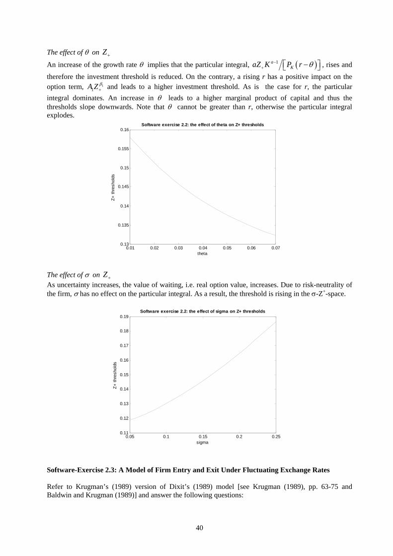
The effect of θ on +ZAn increase of the growth rate θ implies that the particular integral, ( )1a
KaZ K P r θ−+ ⎡ −⎣ ⎤⎦ , rises and
therefore the investment threshold is reduced. On the contrary, a rising r has a positive impact on the option term, 1
1A Z β+ and leads to a higher investment threshold. As is the case for r, the particular
integral dominates. An increase in θ leads to a higher marginal product of capital and thus the thresholds slope downwards. Note that θ cannot be greater than r, otherwise the particular integral explodes.
0.01 0.02 0.03 0.04 0.05 0.06 0.070.13
0.135
0.14
0.145
0.15
0.155
0.16
theta
Z+ th
resh
olds
Software exercise 2.2: the effect of theta on Z+ thresholds
The effect of σ on +ZAs uncertainty increases, the value of waiting, i.e. real option value, increases. Due to risk-neutrality of the firm, σ has no effect on the particular integral. As a result, the threshold is rising in the σ-Z+-space.
0.05 0.1 0.15 0.2 0.250.11
0.12
0.13
0.14
0.15
0.16
0.17
0.18
0.19
sigma
Z+ th
resh
olds
Software exercise 2.2: the effect of sigma on Z+ thresholds
Software-Exercise 2.3: A Model of Firm Entry and Exit Under Fluctuating Exchange Rates Refer to Krugman’s (1989) version of Dixit’s (1989) model [see Krugman (1989), pp. 63-75 and Baldwin and Krugman (1989)] and answer the following questions:
40

(a) Formulate the sunk-cost hysteresis framework and derive the firm’s optimal export supply function in the presence of exchange rate uncertainty and sunk costs.
(b) Demonstrate the dependence of the “hysteresis band” upon the volatility of the exchange rate and the magnitude of the sunk costs.
(c) Rewrite the model assuming that firms cannot drop out of the market at zero cost. How does the introduction of sunk exit costs influence the persistence of producer´s export status?
Subquestion (a): The firm must spend an irrecoverable sunk cost F in domestic currency to enter an export market. On the contrary, the firm can drop out of the market at cost zero. Once in the market, plants are assumed to freely adjust export levels in response to current market conditions. P denotes the (constant) revenue in foreign currency. The exchange rate is a random variable, and hence P is a stochastic variable in domestic currency. To keep the model simple, it is useful to work with the logarithm of the revenues received from exports. Krugman (1989) denotes this in lower capital letters as p. The firm´s operating surplus is then (2.248) , 1−= epπ where the variable costs in domestic currency are normalised to 1. The (risk-neutral) interest rate is r. The exchange rate and therefore the price p is assumed to follow a continuous time diffusion process (2.249) dWdp σ= , where W is a Wiener process. Note, that it is the logarithm of P, not P itself, that follows a random walk. Given this (minimal) framework, the firm has to decide (a) when to invest the irrecoverable sunk cost F and enter the foreign market, and (b) when to exit. We solve this by defining the value function, VI(p), representing the value to be in the market, and another value function, VO(p), that defines how much it is worth to be out. The firm will abandon its capital and exit the market at some p0 at which (2.250) ( ) ( )pVpV IO
00 = . Conversely, the firm will invest the fixed cost F and enter the market at some pI at which (2.251) ( ) ( ) FpVpV I
OI
I += . We now have to determine the forms of the two value functions. The easiest way to proceed is to recognise that the value of being in the market is a kind of an asset, which must offer a competitive return:
(2.252) ( ) ( ) ( )⎥⎦⎤
⎢⎣⎡+−=
dtpdVEepVr Ip
I 1
and
(2.253) ( ) ( )⎥⎦⎤
⎢⎣⎡=
dtpdVEpVr O
O .
But what are these expectations? We can write
41

(2.254)
( ) ( ) ( )( ) ( ) ( )( )
( ) ( ) ( ) ( ) ( ) ( ) ( ) ( )
( ) ( )σ
σ
2
22
2
21
2121
21
pVt
tpVt
pEpVpEpV
tppVppV
EtpVpV
E
I
tIttIttI
tItIt
tIttIt
′′=Δ
Δ′′=
Δ
+Δ′′+Δ′=
⎥⎥⎦
⎤
⎢⎢⎣
⎡
Δ
+Δ′′+Δ′=⎥
⎦
⎤⎢⎣
⎡Δ
−Δ+
LL
L
because the derivative is defined as the limit of the quotient above as Δt → 0. Thus, the differential equations for the value functions as functions of the state variable p are
(2.255) ( ) ( ) ( )rpV
repV I
p
I 21 2σ′′+
−=
and
(2.256) ( ) ( )rpVpV O
O 2
2σ′′= .
The solutions to (2.255) are denoted by
(2.257) ( ) prprp
I BeAerr
epV22 22
2
12
σσ
σ−++−
−=
where the particular solutions can be derived following the solution method in exercise 2.2. We obtain
(2.258) ( ) ( )rr
edsePeEPPppdseeEp
rssrsp 12
1,1 20
2
000
2
−−
=⎥⎦
⎤⎢⎣
⎡−=⎥
⎦
⎤⎢⎣
⎡==− ∫∫
∞−
∞−
σσ ,
since by Ito’s Lemma or by (2.88), ( ) ,22 PdWPdtdP σσ += ; the general solution takes the exponential form of
Pe p =( ) ( ) II VprV ''22σ= .
The general solutions for (2.256) are denoted by
(2.259) ( ) DeCepV prprO σσ 22 22 −+= .
We can further simplify the equations (2.258) and (2.259) by invoking boundary conditions. The deviation of the valuation from the fundamental value [the first term in (2.258)] must be bounded in absolute value. Since p can rise without limit, we must have A = 0. The economic interpretation is that when p is very large, then the value of being in the market should be near its fundamental value. In the same vein, at arbitrarily low values of p, the value of being out of the market should be near zero and therefore D must be zero. So we have
(2.260) ( ) prp
I Berr
epV22
2
12
σ
σ−+−
−=
and
42

(2.260) ( ) CepV prO σ 22= .
Furthermore, we have the boundary conditions for the states in which the firm enters and exists the market: (2.261) ( ) ( )pVpV IO
00 = . (2.262) ( ) ( ) FpVpV I
OI
I += . But we have four unkowns – B, C, pO and pI – and only two equilibrium conditions. We need two more equilibrium conditions and therefore draw on the smooth pasting conditions that come from the requirement that pO and pI be not just points at which the firm switches from being in to out and from out to in, but that they must be the optimal points at which to exit and enter. Not only must the value functions be equal at those two points, they must be tangential. (2.263) ( ) ( )pVpV I
OI
I ′=′ . (2.264) ( ) ( )pVpV O
OO
I ′=′ . In the framework above, sunk costs affect the export supply function for several reasons. First, once a firm has entered a foreign market, a producer will remain in that market as long as operating costs are covered. This implies that exchange rate fluctuations can permanently alter the market structure. For example, devaluations that induce entry into a foreign market may permanently increase exports, even if the currency subsequently appreciates. Second, even if current conditions appear favorable to exporting, they may not induce entry into the foreign market if they are regarded as transitory and the expected future stream of profits may not cover the sunk costs F. In other words, the combination of uncertainty and sunk costs creates an option value of waiting. Equations (2.261) - (2.264) are four non-linear equations with 4 unknown variables. It is easy to solve by the “fsolve” in Matlab. The non-linear equations (2.261) - (2.264) are shown in “fun_Exercise_2_3.m” as a function. The following three “m” files are used:
• “main_Exercise_2_3_f2.m” to replicate the figure 2 of Krugman (1989); • “main_Exercise_2_3.m” to show the effect of F on P ( Pp ln= ) and the effect of sigma on P
( ); Pp ln= The results of main_Exercise_2_3_f2.m: Students need to change/modify the following input data % beginning of input data r =0.08; %benchmark value of Krugman F = 0.8; %benchmark value of Krugman variance = 0.03; %benchmark value of Krugman % end of input data The Matlab program then automatically provides us with the input and output for the optimal point: input data: r sigma F 0.08000 0.17321 0.80000
43

optimal value: pI pO B C 0.29137 -0.25439 1.59392 4.13383 And produces the following figure:
-0.4 -0.3 -0.2 -0.1 0 0.1 0.2 0.3 0.41
2
3
4
5
6
7
8
9
10
11
p
VI:
Bla
ck; V
O: -
-red
Krugman, figure 2
Note that there are two momentous typos on pp. 74-75 of Krugman (1989):
• (A.24) should be ( )[ ] OOO ppp CeBeer ρρ ρρσ =−− −21 2 ,
• (A.26) should be ( )[ ] III ppp CeBeer ρρ ρρσ =−− −21 2 , Moreover, note that the above figure differs slightly different from that of Krugman (1989). The reason for this is a programming error in Krugman´s textbook. The results of main_Exercise_2_3.m: Students need to change/modify the following input data % beginning of input data r =0.08; %benchmark value of Krugman F = 0.8; %benchmark value of Krugman variance = 0.03; %benchmark value of Krugman SC = 0.0; % sunk cost for opting out of market, only 2.3 (c) choiceofplot = 1; % "1" for plot of F; % "2" for plot of sigma; % "3" for plot of SC, for exercise 2.3 (c); % end of input data Given the choice of the value of choiceofplot, 1 or 2 or 3, the matlab m file will generate a plot that shows the effect of F or σ and SC on the investment thresholds, . +Z
44

The effect of F on P thresholds After executing with choiceofplot = 1, the Matlab program automatically provides us with the following figure of the impact of changes in F on the thresholds for P, where . The increase in F has a direct effect on the thresholds of investing, . However, the effect of F on is indirect via
Pp ln=IP OP
( )OIV p .
0.2 0.4 0.6 0.8 1 1.2 1.4 1.6 1.8 2 2.20.7
0.8
0.9
1
1.1
1.2
1.3
1.4
1.5
1.6
F
PI:
blac
k; P
O: -
-red
Software exercise 2.3: the effect of F on P thresholds
The effect of σ on P thresholds After executing with choiceofplot = 2, the Matlab program automatically provides us with the following figure of the impact of changes in σ on the thresholds for P, where . The value of Pp ln=σ exerts its influence via the homogenous solutions. The higher the value of σ , the wider the inaction area is.
0.05 0.1 0.15 0.2 0.25
0.8
1
1.2
1.4
1.6
1.8
2
sigma
PI:
blac
k; P
O: -
-red
Software exercise 2.3: the effect of sigma on P thresholds
(c) The introduction of sunk costs associated with dropping out of the market would lead to changes in (2.261):
45
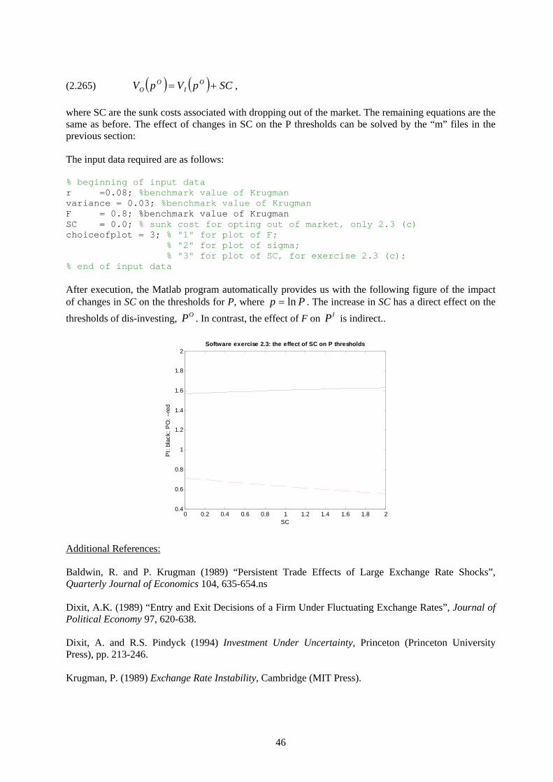
(2.265) ( ) ( ) SCpVpV O
IO
O += , where SC are the sunk costs associated with dropping out of the market. The remaining equations are the same as before. The effect of changes in SC on the P thresholds can be solved by the “m” files in the previous section: The input data required are as follows: % beginning of input data r =0.08; %benchmark value of Krugman variance = 0.03; %benchmark value of Krugman F = 0.8; %benchmark value of Krugman SC = 0.0; % sunk cost for opting out of market, only 2.3 (c) choiceofplot = 3; % "1" for plot of F; % "2" for plot of sigma; % "3" for plot of SC, for exercise 2.3 (c); % end of input data After execution, the Matlab program automatically provides us with the following figure of the impact of changes in SC on the thresholds for P, where Pp ln= . The increase in SC has a direct effect on the thresholds of dis-investing, . In contrast, the effect of F on is indirect.. OP IP
0 0.2 0.4 0.6 0.8 1 1.2 1.4 1.6 1.8 20.4
0.6
0.8
1
1.2
1.4
1.6
1.8
2
SC
PI:
blac
k; P
O: -
-red
Software exercise 2.3: the effect of SC on P thresholds
Additional References: Baldwin, R. and P. Krugman (1989) “Persistent Trade Effects of Large Exchange Rate Shocks”, Quarterly Journal of Economics 104, 635-654.ns Dixit, A.K. (1989) “Entry and Exit Decisions of a Firm Under Fluctuating Exchange Rates”, Journal of Political Economy 97, 620-638. Dixit, A. and R.S. Pindyck (1994) Investment Under Uncertainty, Princeton (Princeton University Press), pp. 213-246. Krugman, P. (1989) Exchange Rate Instability, Cambridge (MIT Press).
46

Software-Exercise 2.4: A Simple Numerical Method – The Euler Scheme for the Geometrical Brownian Motion and the Ornstein-Uhlenbeck process (a) Explain the Poisson process and calculate the jump probabilities of the Poisson process. (b) Modify software exercise 2.2 by using a geometrical Brownian motion combined with two jump
processes (one up and one down) for the path of Z according to
21 ττσθ ddZdWZdtdZ +++= ,
where W is a Wiener process; dtdW ε= (since ε is a normally distributed random variable with mean zero and a standard deviation of unity), η is the drift parameter, σ the variance parameter, dτ1 and dτ2 are the increments of Poisson processes (with mean arrival rates λ1 and λ2). It is assumed that if an “event 1” (“event 2”) occurs, Z increases (falls) by φ1 (φ2) percent with probability 1. Over each time interval dt there is a probability λ1dt (or λ2dt) that it will rise (drop) by φ1Z (φ2Z) and Z fluctuates until next event occurs. Additionally, we assume that (dτ1, dτ2) and dW are independent to each other, i.e. ( ) 01 =τdWdE , ( ) 02 =τdWdE , and E(dτ1dτ2) = 0. Derive the value-matching and smooth-pasting conditions.
(c) Show the impacts of changes in φ1 and φ2 on the thresholds of investment. Solutions: Subquestion (a): The Poisson process implies that the (exogenous) likelihood of a jump is determined by the arrival rate λ. This means that the time t one has to wait for the jump to occur is a random variable whose distribution is exponential with parameter λ: (2.266) { } e ttbeforeoccurseventprobtF λ−−=≡ 1)( The corresponding probability density is (2.267) e ttFtf λ λ−=′≡ )()( In other words, the probability that the jump will occur sometime within the short interval between t0 and t0+dt is approximately λe-λtdt. In particular, the probability that it will occur within dt from now (when t = 0) is approximately λdt. In this sense λ is the probability per unit of time. Moreover, the number of changes (x) that will take place over any interval of length Δ is distributed according to the Poisson distribution
(2.268) { } ( )!
)(x
occureventxprobxg ex Δ−Δ=≡
λλ
whose expected value is the arrival rate times the length of the interval λΔ. As a guide to calibration, the table below provides the probabilities that either one (x = 1) or three (x = 3) jumps will occur within 5 years (Δ = 5) or 10 years (Δ = 10) for the three arrival rates λ = 0.01, λ = 0.05 and λ = 0.10, respectively. For example, for λ = 0.05 the probability that one jump will occur within 5 years is 19.5 percent.
47

Jump Probabilities for the Poisson Process
λ = 0.01 λ = 0.05 λ = 0.10 prob{1 event in 5 years} 0.048 0.195 0.303 prob{3 events in 5 years} 0.000002 0.002 0.013 prob{1 event in 10 years} 0.090 0.303 0.368 prob{3 events in 10 years} 0.0001 0.012 0.061
Subquestion (b): Z follows a geometrical Brownian motion combined with jump processes (2.269) 21 ττσθ ddZdWZdtdZ +++= , Equation (2.269) indicates that there are two sources of uncertainty. Type I uncertainty arises from the geometric Brownian motion while type II uncertainty arises from the jump processes. The partial differential equation (2.57) in the textbook now is
(2.270) ( ) ( ) ( ) ( )
( )( ) ( )( )
22 2
2
1 1 2 2
' , 1,2
1 1 .k
F K Z q K Z q K Zrq K Z Z Z Z
P Z Z
q Z q q q Z
θ θ σ
λ φ λ φ
∂ ∂= + +
∂ ∂
⎡ ⎤ ⎡+ + − − − −⎣ ⎦ ⎣
,
⎤⎦
The last two terms represent the changes of q caused by positive jumps and negative drops, respectively. The solutions for (2.270) again consist of the particular and homogenous solutions. For the particular solutions, we can guess a solution 1P aq ZKφ −= and obtain
(2.271) ( )
1
1 1 2 2
.a
P
K
aZKqP r θ λφ λ φ
−
=− − +
The homogeneous part of the Bellman’s equation is denoted by
(2.272) ( )( ) ( )( )2
21 1 21 1
2H H H H H H H
Z ZZrq Zq Z q q Z q q q Zσθ λ φ λ 2φ⎡ ⎤ ⎡= + + + − − − − ⎤⎣ ⎦ ⎣ ⎦ .
Assume the homogeneous solutions have the functional form, ( )1H aq A ZKβ−= , as in exercise 2.2. We
then have the characteristic equation
(2.273) ( ) ( ) ( )21 1 2 2
1 1 1 1 1 12
rβ βσ β β θβ λ φ λ φ⎡ ⎤ ⎡ ⎤− + + + − − − − − =⎣ ⎦ ⎣ ⎦ 0 .
There are two roots to the above equations, one positive and one negative. Assume that 1 0β > and
2 0β < . Thus, the homogenous solutions, representing the option values, become
(2.274) ( ) ( )1 21 11 2
H a aq A ZK A ZKβ β− −= + ,
which is the same as (2.239) except for the value of betas. Since there is no depreciation and therefore the capital stock is predetermined, the above equation can be simplified as
48
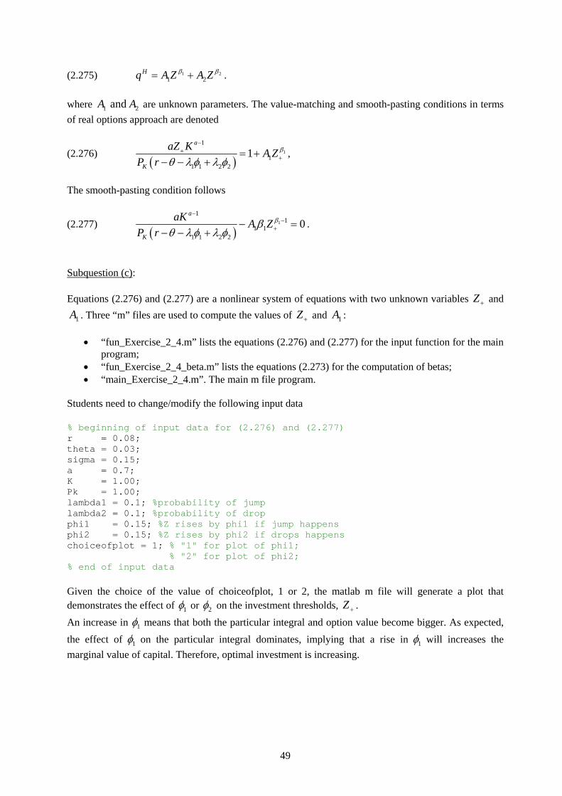
(2.275) 1 21 2
Hq A Z A Zβ β= + . where are unknown parameters. The value-matching and smooth-pasting conditions in terms of real options approach are denoted
1 and A 2A
(2.276) ( )
1
1
11 1 2 2
1a
K
aZ K A ZP r
β
θ λφ λ φ
−+
+= +− − +
,
The smooth-pasting condition follows
(2.277) ( )
1
11
1 11 1 2 2
0a
K
aK A ZP r
ββθ λφ λ φ
−−
+− =− − +
.
Subquestion (c): Equations (2.276) and (2.277) are a nonlinear system of equations with two unknown variables and
. Three “m” files are used to compute the values of and : +Z
1A +Z 1A
• “fun_Exercise_2_4.m” lists the equations (2.276) and (2.277) for the input function for the main program;
• “fun_Exercise_2_4_beta.m” lists the equations (2.273) for the computation of betas; • “main_Exercise_2_4.m”. The main m file program.
Students need to change/modify the following input data % beginning of input data for (2.276) and (2.277) r = 0.08; theta = 0.03; sigma = 0.15; a = 0.7; K = 1.00; Pk = 1.00; lambda1 = 0.1; %probability of jump lambda2 = 0.1; %probability of drop phi1 = 0.15; %Z rises by phi1 if jump happens phi2 = 0.15; %Z rises by phi2 if drops happens choiceofplot = 1; % "1" for plot of phi1; % "2" for plot of phi2; % end of input data Given the choice of the value of choiceofplot, 1 or 2, the matlab m file will generate a plot that demonstrates the effect of 1φ or 2φ on the investment thresholds, . +ZAn increase in 1φ means that both the particular integral and option value become bigger. As expected, the effect of 1φ on the particular integral dominates, implying that a rise in 1φ will increases the marginal value of capital. Therefore, optimal investment is increasing.
49

0 0.02 0.04 0.06 0.08 0.1 0.12 0.14 0.16 0.18 0.20.15
0.151
0.152
0.153
0.154
0.155
0.156
0.157
0.158
0.159
phi1
Z+ th
resh
olds
Software exercise 2.4: the effect of phi1 on Z+ thresholds
An increase in 2φ implies that the negative shocks are bigger in magnitude and therefore the implied risk is larger. Thus, both the particular integral and option value become smaller. Again, the effect of
2φ on the particular integral dominates. Hence, the rise in 2φ will lead to a lower marginal value of capital and the firm is more reluctant to invest.
0 0.02 0.04 0.06 0.08 0.1 0.12 0.14 0.16 0.18 0.20.14
0.142
0.144
0.146
0.148
0.15
0.152
0.154
0.156
0.158
phi2
Z+ th
resh
olds
Software exercise 2.4: the effect of phi2 on Z+ thresholds
50