chapter 2: demand theory - faculty.ses.wsu.edufaculty.ses.wsu.edu/espinola/demand...
TRANSCRIPT
Demand Theory
Utility Maximization Problem
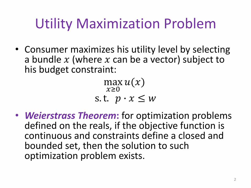
• Consumer maximizes his utility level by selecting a bundle 𝑥 (where 𝑥 can be a vector) subject to his budget constraint:
max𝑥≥0
𝑢(𝑥)
s. t. 𝑝 ∙ 𝑥 ≤ 𝑤
• Weierstrass Theorem: for optimization problems defined on the reals, if the objective function is continuous and constraints define a closed and bounded set, then the solution to such optimization problem exists.
2
Utility Maximization Problem
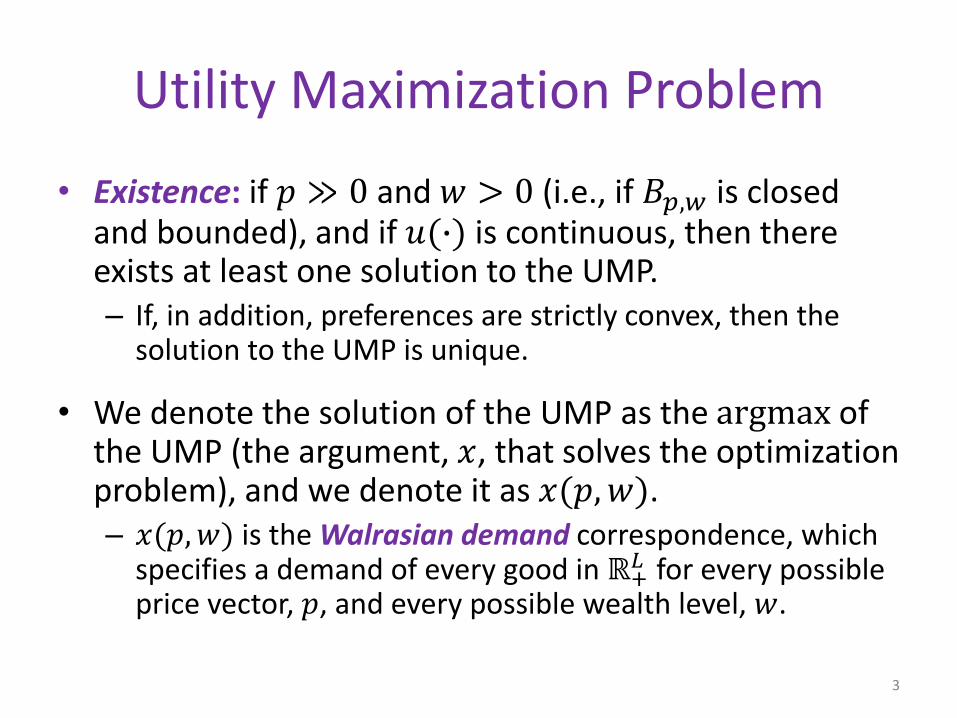
• Existence: if 𝑝 ≫ 0 and 𝑤 > 0 (i.e., if 𝐵𝑝,𝑤 is closed and bounded), and if 𝑢(∙) is continuous, then there exists at least one solution to the UMP.– If, in addition, preferences are strictly convex, then the
solution to the UMP is unique.
• We denote the solution of the UMP as the argmax of the UMP (the argument, 𝑥, that solves the optimization problem), and we denote it as 𝑥(𝑝, 𝑤). – 𝑥(𝑝, 𝑤) is the Walrasian demand correspondence, which
specifies a demand of every good in ℝ+𝐿 for every possible
price vector, 𝑝, and every possible wealth level, 𝑤.
3
Utility Maximization Problem
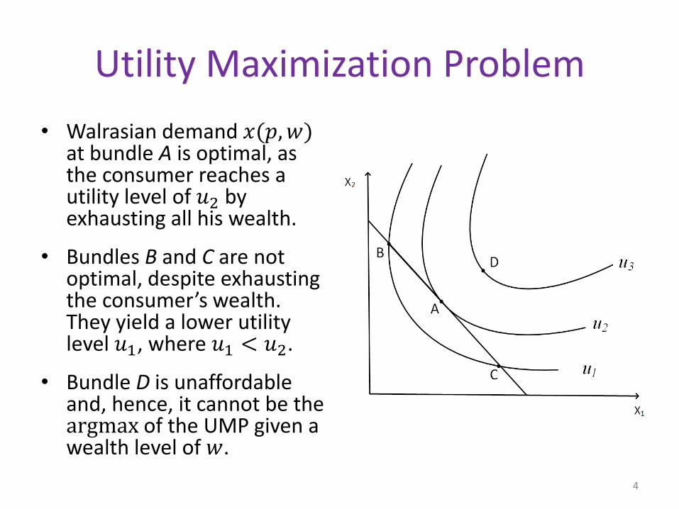
• Walrasian demand 𝑥(𝑝, 𝑤)at bundle A is optimal, as the consumer reaches a utility level of 𝑢2 by exhausting all his wealth.
• Bundles B and C are not optimal, despite exhausting the consumer’s wealth. They yield a lower utility level 𝑢1, where 𝑢1 < 𝑢2.
• Bundle D is unaffordable and, hence, it cannot be the argmax of the UMP given a wealth level of 𝑤.
4
Properties of Walrasian Demand
• If the utility function is continuous and preferences satisfy LNS over the consumption set 𝑋 = ℝ+
𝐿 , then the Walrasian demand 𝑥(𝑝, 𝑤) satisfies:
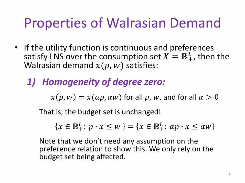
1) Homogeneity of degree zero:
𝑥 𝑝, 𝑤 = 𝑥(𝛼𝑝, 𝛼𝑤) for all 𝑝, 𝑤, and for all 𝛼 > 0
That is, the budget set is unchanged!
𝑥 ∈ ℝ+𝐿 : 𝑝 ∙ 𝑥 ≤ 𝑤 = 𝑥 ∈ ℝ+
𝐿 : 𝛼𝑝 ∙ 𝑥 ≤ 𝛼𝑤
Note that we don’t need any assumption on the preference relation to show this. We only rely on the budget set being affected.
5
x1
x2
wp2
α wα p2
=
wp1
α wα p1
=
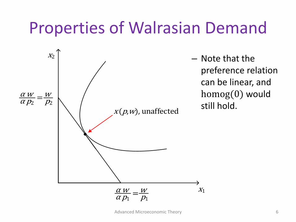
x (p,w), unaffected
Properties of Walrasian Demand
Advanced Microeconomic Theory 6
– Note that the preference relation can be linear, and homog(0) would still hold.
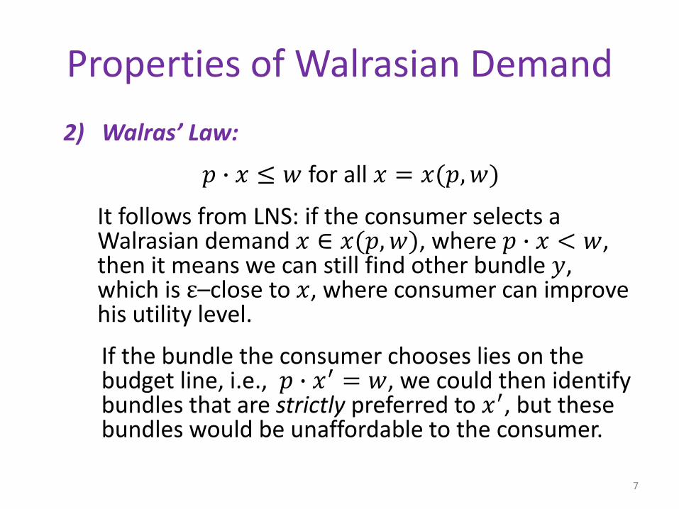
2) Walras’ Law:
𝑝 ∙ 𝑥 ≤ 𝑤 for all 𝑥 = 𝑥(𝑝, 𝑤)
It follows from LNS: if the consumer selects a Walrasian demand 𝑥 ∈ 𝑥(𝑝, 𝑤), where 𝑝 ∙ 𝑥 < 𝑤, then it means we can still find other bundle 𝑦, which is ε–close to 𝑥, where consumer can improve his utility level.
If the bundle the consumer chooses lies on the budget line, i.e., 𝑝 ∙ 𝑥′ = 𝑤, we could then identify bundles that are strictly preferred to 𝑥′, but these bundles would be unaffordable to the consumer.
Properties of Walrasian Demand
7
x
x2
x1
Properties of Walrasian Demand
8
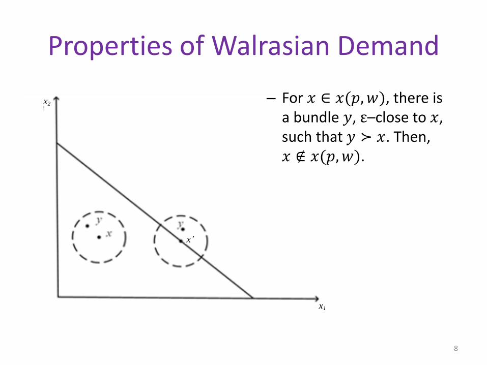
– For 𝑥 ∈ 𝑥(𝑝, 𝑤), there is a bundle 𝑦, ε–close to 𝑥, such that 𝑦 ≻ 𝑥. Then, 𝑥 ∉ 𝑥(𝑝, 𝑤).
Properties of Walrasian Demand
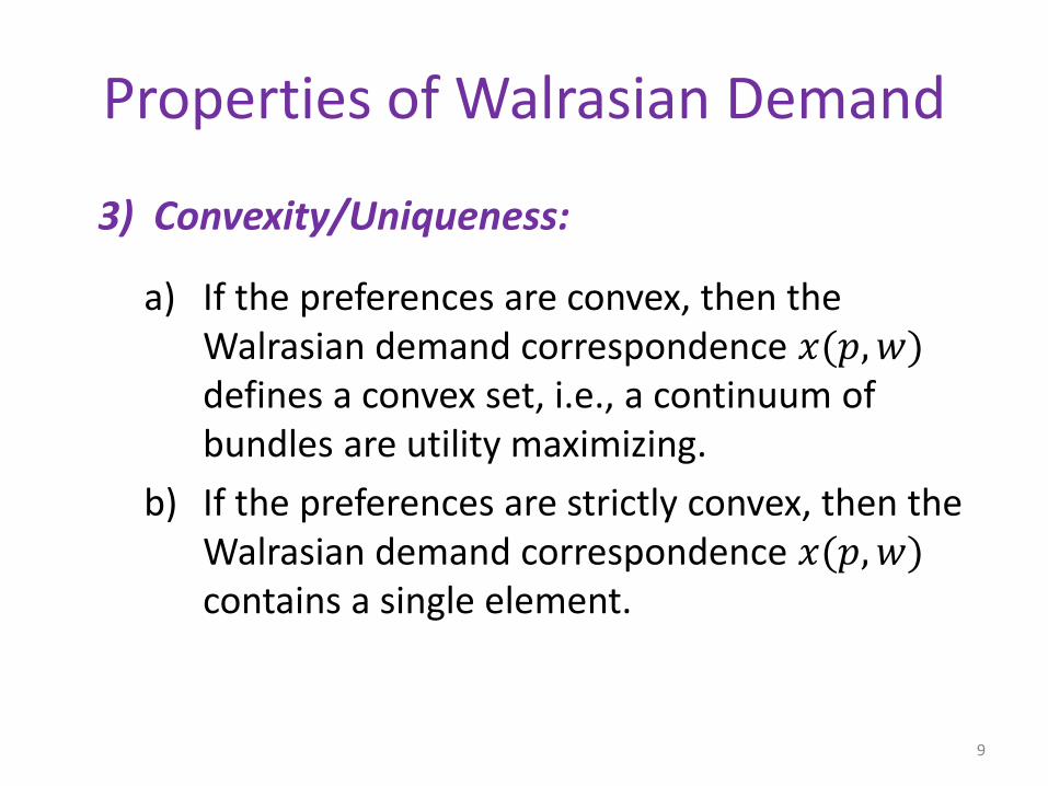
3) Convexity/Uniqueness:
a) If the preferences are convex, then the Walrasian demand correspondence 𝑥(𝑝, 𝑤)defines a convex set, i.e., a continuum of bundles are utility maximizing.
b) If the preferences are strictly convex, then the Walrasian demand correspondence 𝑥(𝑝, 𝑤)contains a single element.
9
Properties of Walrasian Demand
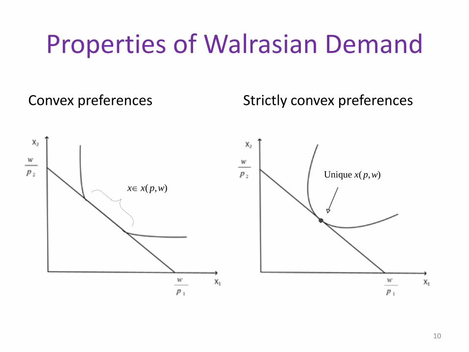
Convex preferences Strictly convex preferences
10
( , )x x p w
Unique ( , )x p w

UMP: Necessary Condition
max𝑥≥0
𝑢 𝑥 s. t. 𝑝 ∙ 𝑥 ≤ 𝑤
• We solve it using Kuhn-Tucker conditions over the Lagrangian 𝐿 = 𝑢 𝑥 + 𝜆(𝑤 − 𝑝 ∙ 𝑥),
𝜕𝐿
𝜕𝑥𝑘=
𝜕𝑢(𝑥∗)
𝜕𝑥𝑘− 𝜆𝑝𝑘 ≤ 0 for all 𝑘, = 0 if 𝑥𝑘
∗ > 0
𝜕𝐿
𝜕𝜆= 𝑤 − 𝑝 ∙ 𝑥∗ = 0
• That is in the interior optimum, 𝜕𝑢(𝑥∗)
𝜕𝑥𝑘= 𝜆𝑝𝑘 for every
good 𝑘, which implies𝜕𝑢(𝑥∗)
𝜕𝑥𝑙𝜕𝑢(𝑥∗)
𝜕𝑥𝑘
=𝑝𝑙
𝑝𝑘⇔ 𝑀𝑅𝑆 𝑙,𝑘 =
𝑝𝑙
𝑝𝑘⇔
𝜕𝑢(𝑥∗)
𝜕𝑥𝑙
𝑝𝑙=
𝜕𝑢(𝑥∗)
𝜕𝑥𝑘
𝑝𝑘
11

UMP: Sufficient Condition
• When are Kuhn-Tucker (necessary) conditions, also sufficient?
– That is, when can we guarantee that 𝑥(𝑝, 𝑤) is the max of the UMP and not the min?
• Answer: if 𝑢(∙) is quasiconcave and monotone, and has Hessian 𝛻𝑢(𝑥) ≠ 0 for 𝑥 ∈ ℝ+
𝐿 , then the Kuhn-Tucker FOCs are also sufficient.
12
UMP: Sufficient Condition
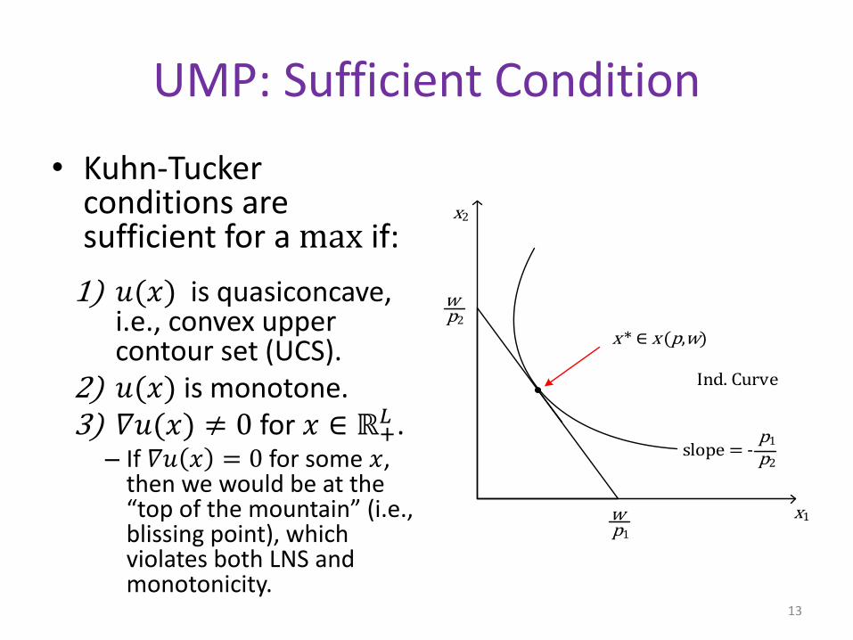
• Kuhn-Tucker conditions are sufficient for a max if:
1) 𝑢(𝑥) is quasiconcave, i.e., convex upper contour set (UCS).
2) 𝑢(𝑥) is monotone.3) 𝛻𝑢(𝑥) ≠ 0 for 𝑥 ∈ ℝ+
𝐿 .– If 𝛻𝑢 𝑥 = 0 for some 𝑥,
then we would be at the “top of the mountain” (i.e., blissing point), which violates both LNS and monotonicity.
13
x1
x2
wp2
wp1
x * ∈ x (p,w)
slope = - p2
p1
Ind. Curve
UMP: Violations of Sufficient Condition
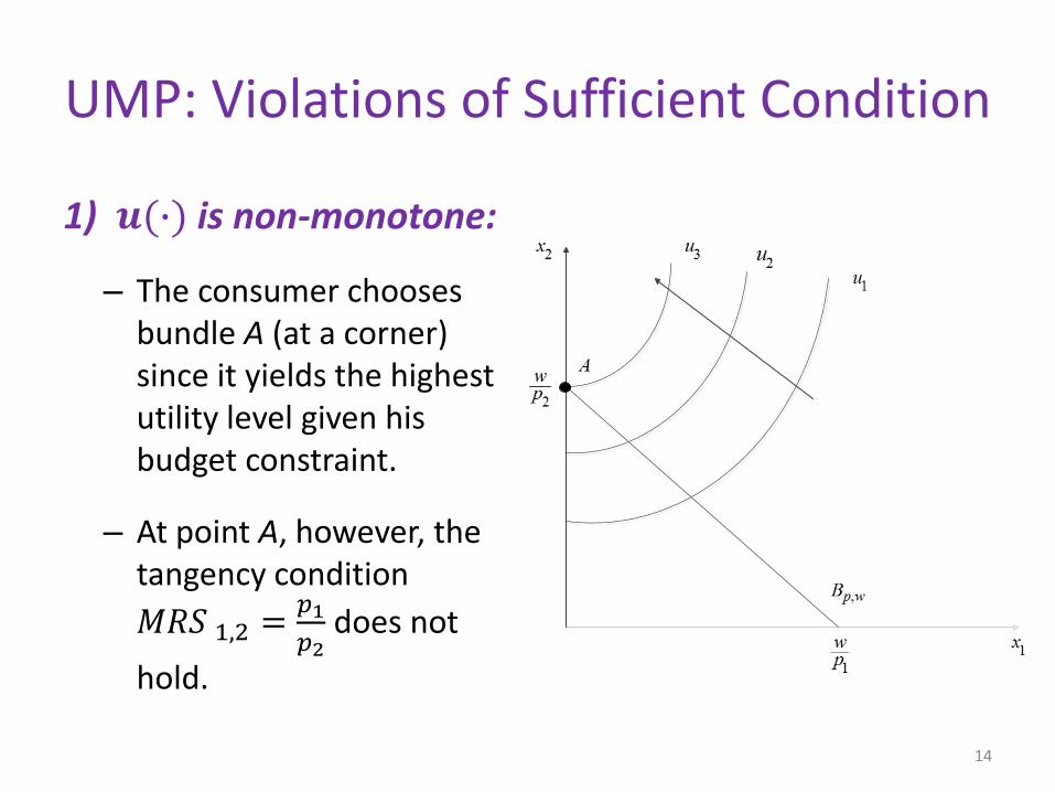
1) 𝒖(∙) is non-monotone:
– The consumer chooses bundle A (at a corner) since it yields the highest utility level given his budget constraint.
– At point A, however, the tangency condition
𝑀𝑅𝑆 1,2 =𝑝1
𝑝2does not
hold.
14
UMP: Violations of Sufficient Condition
15
x2
x1
A
B
C
Budget line
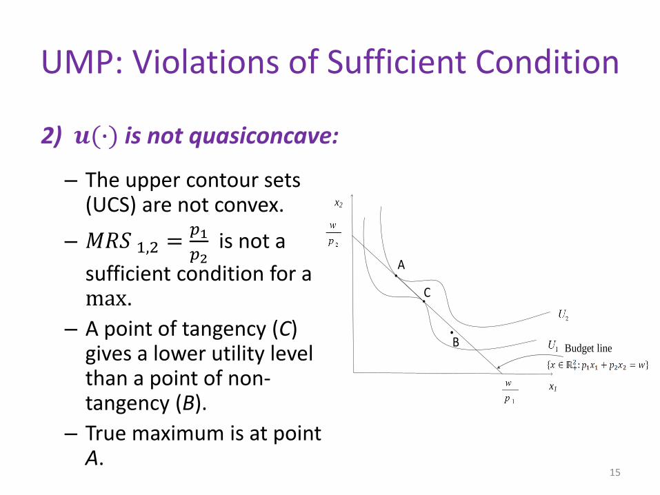
– The upper contour sets (UCS) are not convex.
– 𝑀𝑅𝑆 1,2 =𝑝1
𝑝2is not a
sufficient condition for a max.
– A point of tangency (C) gives a lower utility level than a point of non-tangency (B).
– True maximum is at point A.
2) 𝒖(∙) is not quasiconcave:
UMP: Corner Solution
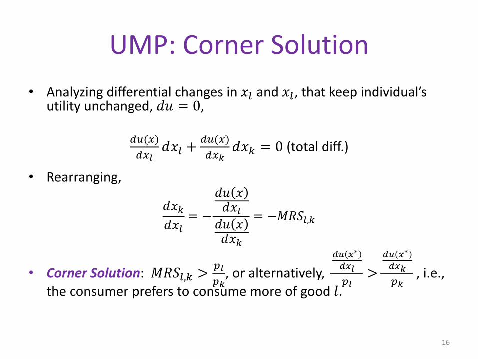
• Analyzing differential changes in 𝑥𝑙 and 𝑥𝑙, that keep individual’s utility unchanged, 𝑑𝑢 = 0,
𝑑𝑢(𝑥)
𝑑𝑥𝑙𝑑𝑥𝑙 +
𝑑𝑢(𝑥)
𝑑𝑥𝑘𝑑𝑥𝑘 = 0 (total diff.)
• Rearranging,
𝑑𝑥𝑘
𝑑𝑥𝑙= −
𝑑𝑢 𝑥𝑑𝑥𝑙
𝑑𝑢 𝑥𝑑𝑥𝑘
= −𝑀𝑅𝑆𝑙,𝑘
• Corner Solution: 𝑀𝑅𝑆𝑙,𝑘 >𝑝𝑙
𝑝𝑘, or alternatively,
𝑑𝑢 𝑥∗
𝑑𝑥𝑙
𝑝𝑙>
𝑑𝑢 𝑥∗
𝑑𝑥𝑘
𝑝𝑘, i.e.,
the consumer prefers to consume more of good 𝑙.
16
UMP: Corner Solution
• In the FOCs, this implies:
a)𝜕𝑢(𝑥∗)
𝜕𝑥𝑘≤ 𝜆𝑝𝑘 for the goods whose consumption is
zero, 𝑥𝑘∗= 0, and
b)𝜕𝑢(𝑥∗)
𝜕𝑥𝑙= 𝜆𝑝𝑙 for the good whose consumption is
positive, 𝑥𝑙∗> 0.
• Intuition: the marginal utility per dollar spent on good 𝑙 is still larger than that on good 𝑘.
𝜕𝑢(𝑥∗)
𝜕𝑥𝑙
𝑝𝑙= 𝜆 ≥
𝜕𝑢(𝑥∗)
𝜕𝑥𝑘
𝑝𝑘
17

UMP: Corner Solution
• Consumer seeks to consume good 1 alone.
• At the corner solution, the indifference curve is steeper than the budget line, i.e.,
𝑀𝑅𝑆1,2 >𝑝1
𝑝2or
𝑀𝑈1
𝑝1>
𝑀𝑈2
𝑝2
• Intuitively, the consumer would like to consume more of good 1, even after spending his entire wealth on good 1 alone.
18
x1
x2
wp2
wp1
slope of the B.L. = - p2
p1
slope of the I.C. = MRS1,2
UMP: Lagrange Multiplier
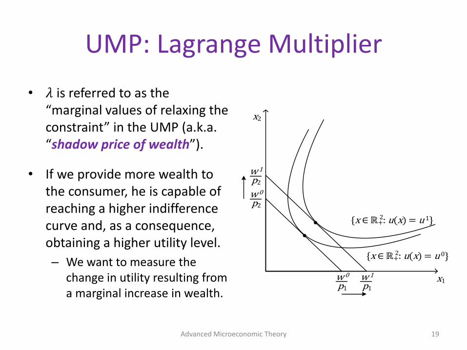
• 𝜆 is referred to as the “marginal values of relaxing the constraint” in the UMP (a.k.a.“shadow price of wealth”).
• If we provide more wealth to the consumer, he is capable of reaching a higher indifference curve and, as a consequence, obtaining a higher utility level.
– We want to measure the change in utility resulting from a marginal increase in wealth.
Advanced Microeconomic Theory 19
x1
x2
w 0
p2
{x +: u(x) = u 1}2
{x +: u(x) = u 0}2
w 1
p2
w 0
p1
w 1
p1
UMP: Lagrange Multiplier
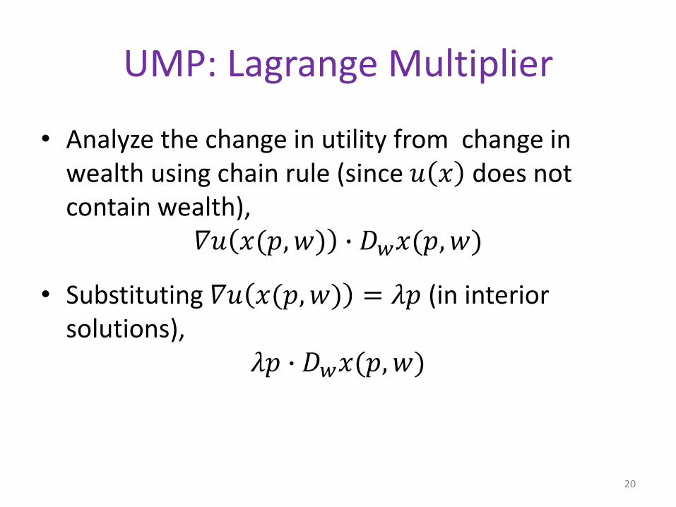
• Analyze the change in utility from change in wealth using chain rule (since 𝑢 𝑥 does not contain wealth),
𝛻𝑢 𝑥(𝑝, 𝑤) ∙ 𝐷𝑤𝑥(𝑝, 𝑤)
• Substituting 𝛻𝑢 𝑥(𝑝, 𝑤) = 𝜆𝑝 (in interior solutions),
𝜆𝑝 ∙ 𝐷𝑤𝑥(𝑝, 𝑤)
20
UMP: Lagrange Multiplier
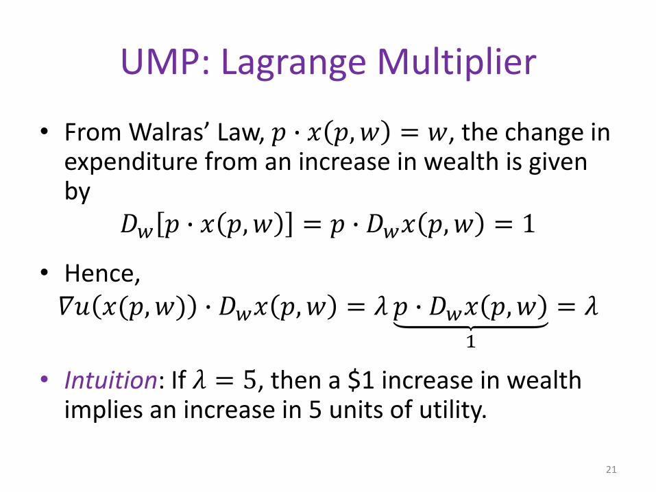
• From Walras’ Law, 𝑝 ∙ 𝑥 𝑝, 𝑤 = 𝑤, the change in expenditure from an increase in wealth is given by
𝐷𝑤 𝑝 ∙ 𝑥 𝑝, 𝑤 = 𝑝 ∙ 𝐷𝑤𝑥 𝑝, 𝑤 = 1
• Hence, 𝛻𝑢 𝑥(𝑝, 𝑤) ∙ 𝐷𝑤𝑥 𝑝, 𝑤 = 𝜆 𝑝 ∙ 𝐷𝑤𝑥 𝑝, 𝑤
1
= 𝜆
• Intuition: If 𝜆 = 5, then a $1 increase in wealth implies an increase in 5 units of utility.
21

Walrasian Demand
• We found the Walrasian demand function, 𝑥 𝑝, 𝑤 , as the solution to the UMP.
• Properties of 𝑥 𝑝, 𝑤 :1) Homog(0), for any 𝑝, 𝑤, 𝛼 > 0,
𝑥 𝛼𝑝, 𝛼𝑤 = 𝑥 𝑝, 𝑤(Budget set is unaffected by changes in 𝑝 and 𝑤 of the same size)
2) Walras’ Law: for every 𝑝 ≫ 0, 𝑤 > 0 we have 𝑝 ∙ 𝑥 = 𝑤 for all 𝑥 ∈ 𝑥(𝑝, 𝑤)
(This is because of LNS)
22

Walrasian Demand: Wealth Effects
• Normal vs. Inferior goods
𝜕𝑥 𝑝,𝑤
𝜕𝑤
><
0 normalinferior
• Examples of inferior goods:
– Two-buck chuck (a really cheap wine)
– Walmart during the economic crisis
23

Walrasian Demand: Wealth Effects
• An increase in the wealth level produces an outward shift in the budget line.
• 𝑥2 is normal as 𝜕𝑥2 𝑝,𝑤
𝜕𝑤> 0, while
𝑥1 is inferior as 𝜕𝑥 𝑝,𝑤
𝜕𝑤< 0.
• Wealth expansion path: – connects the optimal consumption
bundle for different levels of wealth
– indicates how the consumption of a good changes as a consequence of changes in the wealth level
24

Walrasian Demand: Wealth Effects
• Engel curve depicts the consumption of a particular good in the horizontal axis and wealth on the vertical axis.
• The slope of the Engel curve is:
– positive if the good is normal
– negative if the good is inferior
• Engel curve can be positively slopped for low wealth levels and become negatively slopped afterwards.
25
x1
Wealth, w
ŵ
Engel curve for a normal good (up to income ŵ), but inferior
good for all w > ŵ
Engel curve of a normal good, for all w.
Walrasian Demand: Price Effects
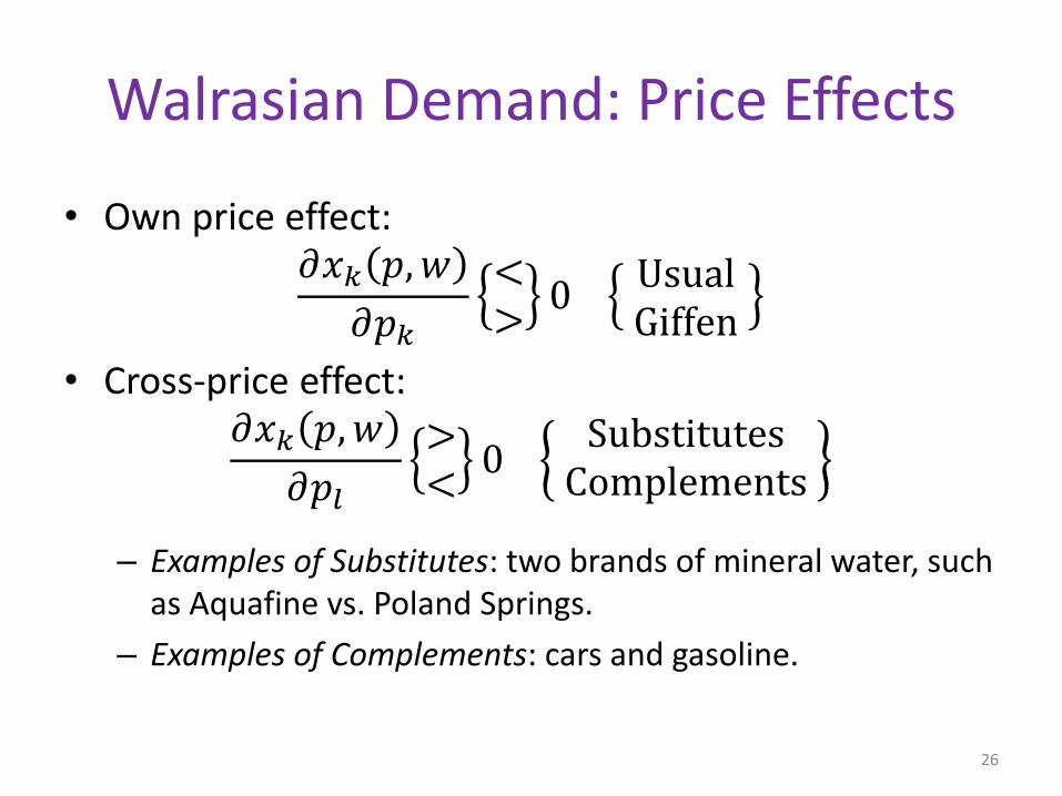
• Own price effect:𝜕𝑥𝑘 𝑝, 𝑤
𝜕𝑝𝑘
<>
0UsualGiffen
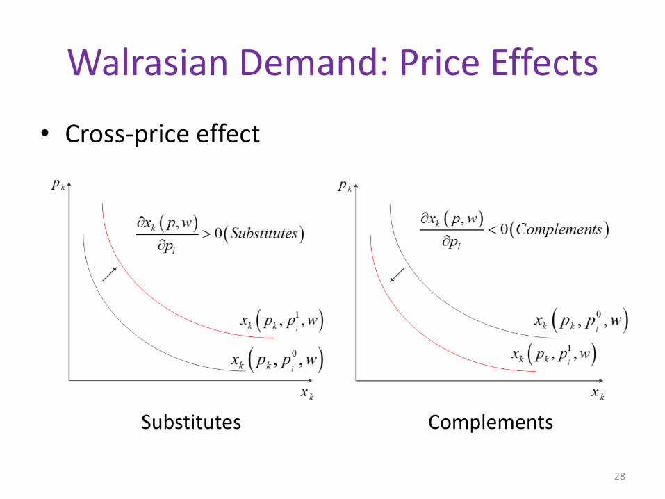
• Cross-price effect:𝜕𝑥𝑘 𝑝, 𝑤
𝜕𝑝𝑙
><
0Substitutes
Complements
– Examples of Substitutes: two brands of mineral water, such as Aquafine vs. Poland Springs.
– Examples of Complements: cars and gasoline.
26

Walrasian Demand: Price Effects
• Own price effect
27
Usual good Giffen good
Walrasian Demand: Price Effects
28
• Cross-price effect
Substitutes Complements
Indirect Utility Function
• The Walrasian demand function, 𝑥 𝑝, 𝑤 , is the solution to the UMP (i.e., argmax).
• What would be the utility function evaluated at the solution of the UMP, i.e., 𝑥 𝑝, 𝑤 ?
– This is the indirect utility function (i.e., the highest utility level), 𝑣 𝑝, 𝑤 ∈ ℝ, associated with the UMP.
– It is the “value function” of this optimization problem.
29

Properties of Indirect Utility Function
• If the utility function is continuous and preferences satisfy LNS over the consumption set 𝑋 = ℝ+
𝐿 , then the indirect utility function 𝑣 𝑝, 𝑤 satisfies:
1) Homogenous of degree zero: Increasing 𝑝 and 𝑤by a common factor 𝛼 > 0 does not modify the consumer’s optimal consumption bundle,𝑥(𝑝, 𝑤), nor his maximal utility level, measured by 𝑣 𝑝, 𝑤 .
30

Properties of Indirect Utility Function
31
x1
x2
wp2
α wα p2
=
wp1
α wα p1
=
x (p,w) = x (αp,α w)
v (p,w) = v (αp,α w)
Bp,w = Bαp,αw
Properties of Indirect Utility Function
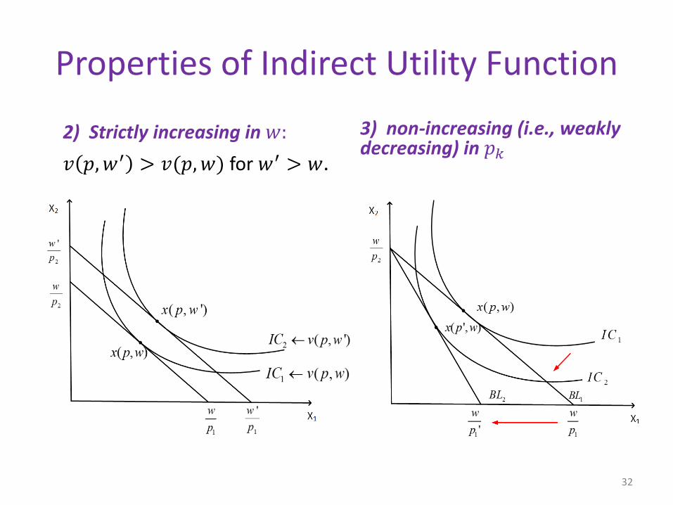
2) Strictly increasing in 𝑤:
𝑣 𝑝, 𝑤′ > 𝑣(𝑝, 𝑤) for 𝑤′ > 𝑤.
3) non-increasing (i.e., weakly decreasing) in 𝑝𝑘
32
Properties of Indirect Utility Function
33
W
P1
w2
w1
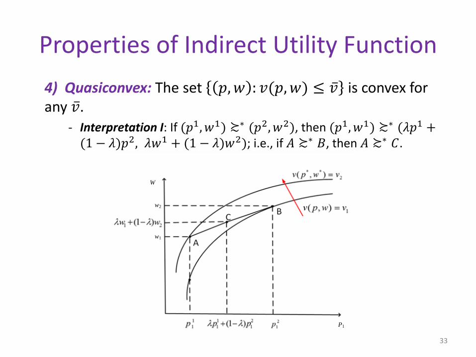
4) Quasiconvex: The set 𝑝, 𝑤 : 𝑣(𝑝, 𝑤) ≤ ҧ𝑣 is convex for any ҧ𝑣.
- Interpretation I: If (𝑝1, 𝑤1) ≿∗ (𝑝2, 𝑤2), then (𝑝1, 𝑤1) ≿∗ (𝜆𝑝1 +(1 − 𝜆)𝑝2, 𝜆𝑤1 + (1 − 𝜆)𝑤2); i.e., if 𝐴 ≿∗ 𝐵, then 𝐴 ≿∗ 𝐶.
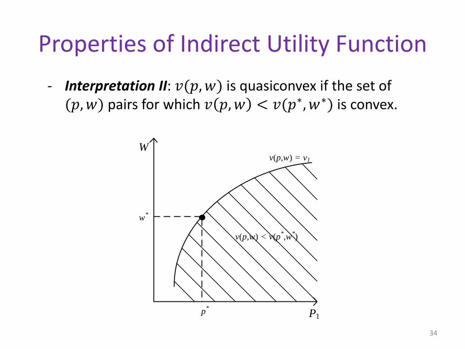
Properties of Indirect Utility Function
- Interpretation II: 𝑣(𝑝, 𝑤) is quasiconvex if the set of (𝑝, 𝑤) pairs for which 𝑣 𝑝, 𝑤 < 𝑣(𝑝∗, 𝑤∗) is convex.
34
W
P1
w*
p*
v(p,w) < v(p*,w
*)
v(p,w) = v1
Properties of Indirect Utility Function
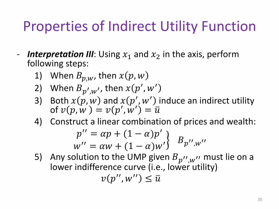
- Interpretation III: Using 𝑥1 and 𝑥2 in the axis, perform following steps:
1) When 𝐵𝑝,𝑤, then 𝑥 𝑝, 𝑤
2) When 𝐵𝑝′,𝑤′, then 𝑥 𝑝′, 𝑤′
3) Both 𝑥 𝑝, 𝑤 and 𝑥 𝑝′, 𝑤′ induce an indirect utility of 𝑣 𝑝, 𝑤 = 𝑣 𝑝′, 𝑤′ = ത𝑢
4) Construct a linear combination of prices and wealth:
ൠ𝑝′′ = 𝛼𝑝 + (1 − 𝛼)𝑝′
𝑤′′ = 𝛼𝑤 + (1 − 𝛼)𝑤′ 𝐵𝑝′′,𝑤′′
5) Any solution to the UMP given 𝐵𝑝′′,𝑤′′ must lie on a lower indifference curve (i.e., lower utility)
𝑣 𝑝′′, 𝑤′′ ≤ ത𝑢
35
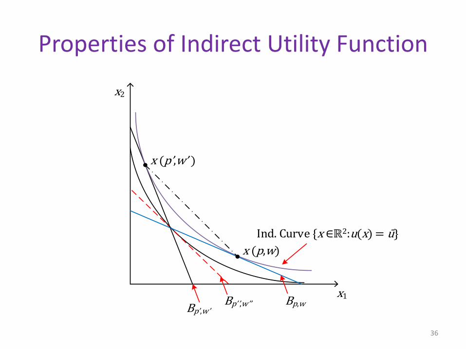
Properties of Indirect Utility Function
36
x1
x2
Bp,wBp’,w’Bp’’,w’’
x (p,w)
x (p’,w’ )
Ind. Curve {x ∈ℝ2:u(x) = ū}
WARP and Walrasian Demand
• Relation between Walrasian demand 𝑥 𝑝, 𝑤and WARP
– How does the WARP restrict the set of optimal consumption bundles that the individual decision-maker can select when solving the UMP?
37

WARP and Walrasian Demand
• Take two different consumption bundles 𝑥 𝑝, 𝑤 and 𝑥 𝑝′, 𝑤′ , both being affordable 𝑝, 𝑤 , i.e.,
𝑝 ∙ 𝑥 𝑝, 𝑤 ≤ 𝑤 and 𝑝 ∙ 𝑥 𝑝′, 𝑤′ ≤ 𝑤
• When prices and wealth are 𝑝, 𝑤 , the consumer chooses 𝑥 𝑝, 𝑤 despite 𝑥 𝑝′, 𝑤′ is also affordable.
• Then he “reveals” a preference for 𝑥 𝑝, 𝑤 over 𝑥 𝑝′, 𝑤′when both are affordable.
• Hence, we should expect him to choose 𝑥 𝑝, 𝑤 over 𝑥 𝑝′, 𝑤′ when both are affordable. (Consistency)
• Therefore, bundle 𝑥 𝑝, 𝑤 must not be affordable at 𝑝′, 𝑤′ because the consumer chooses 𝑥 𝑝′, 𝑤′ . That is,
𝑝′ ∙ 𝑥 𝑝, 𝑤 > 𝑤′.
38
WARP and Walrasian Demand
• In summary, Walrasian demand satisfies WARP, if, for two different consumption bundles, 𝑥 𝑝, 𝑤 ≠ 𝑥 𝑝′, 𝑤′ ,
𝑝 ∙ 𝑥 𝑝′, 𝑤′ ≤ 𝑤 ⇒ 𝑝′ ∙ 𝑥 𝑝, 𝑤 > 𝑤′
• Intuition: if 𝑥 𝑝′, 𝑤′ is affordable under budget set 𝐵𝑝,𝑤, then 𝑥 𝑝, 𝑤 cannot be affordable
under 𝐵𝑝′,𝑤′.
39
Checking for WARP
• A systematic procedure to check if Walrasian demand satisfies WARP:– Step 1: Check if bundles 𝑥 𝑝, 𝑤 and 𝑥 𝑝′, 𝑤′ are
both affordable under 𝐵𝑝,𝑤. That is, graphically 𝑥 𝑝, 𝑤 and 𝑥 𝑝′, 𝑤′ have to lie on
or below budget line 𝐵𝑝,𝑤.
If step 1 is satisfied, then move to step 2.
Otherwise, the premise of WARP does not hold, which does not allow us to continue checking if WARP is violated or not. In this case, we can only say that “WARP is not violated”.
40
Checking for WARP
- Step 2: Check if bundles 𝑥 𝑝, 𝑤 is affordable under 𝐵𝑝′,𝑤′.
That is, graphically 𝑥 𝑝, 𝑤 must lie on or below budge line 𝐵𝑝′,𝑤′.
If step 2 is satisfied, then this Walrasian demand violates WARP.
Otherwise, the Walrasian demand satisfies WARP.
41
Checking for WARP: Example 1
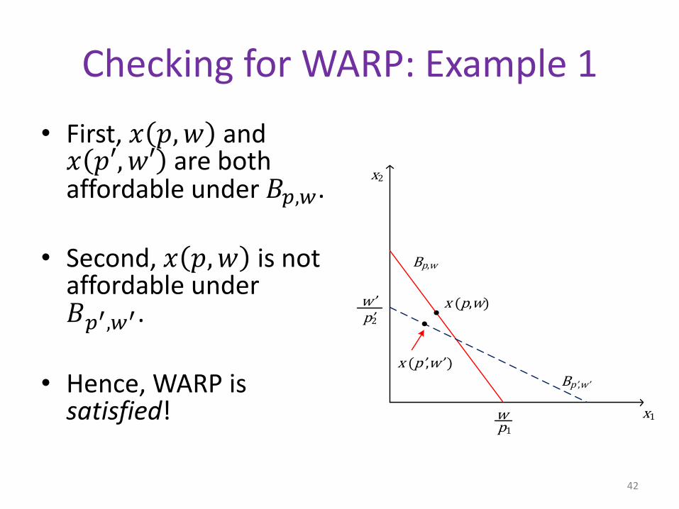
• First, 𝑥 𝑝, 𝑤 and 𝑥 𝑝′, 𝑤′ are both affordable under 𝐵𝑝,𝑤.
• Second, 𝑥 𝑝, 𝑤 is not affordable under 𝐵𝑝′,𝑤′.
• Hence, WARP is satisfied!
42
x1
x2
w p2
wp1
Bp,w
Bp ,w
x (p,w)
x (p ,w )
Checking for WARP: Example 2
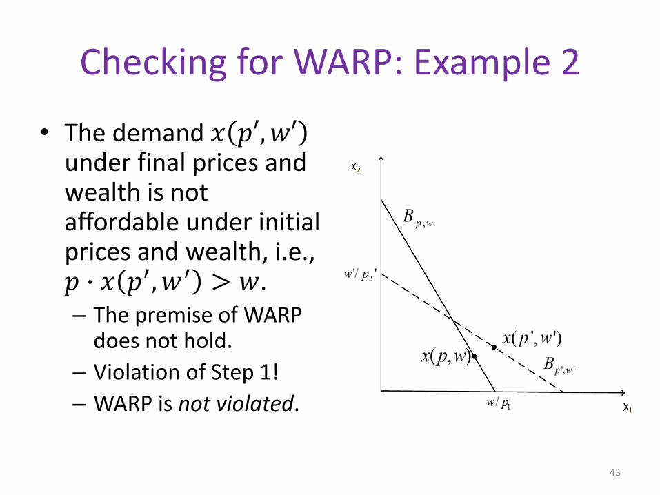
• The demand 𝑥 𝑝′, 𝑤′under final prices and wealth is not affordable under initial prices and wealth, i.e., 𝑝 ∙ 𝑥 𝑝′, 𝑤′ > 𝑤.– The premise of WARP
does not hold.
– Violation of Step 1!
– WARP is not violated.
43
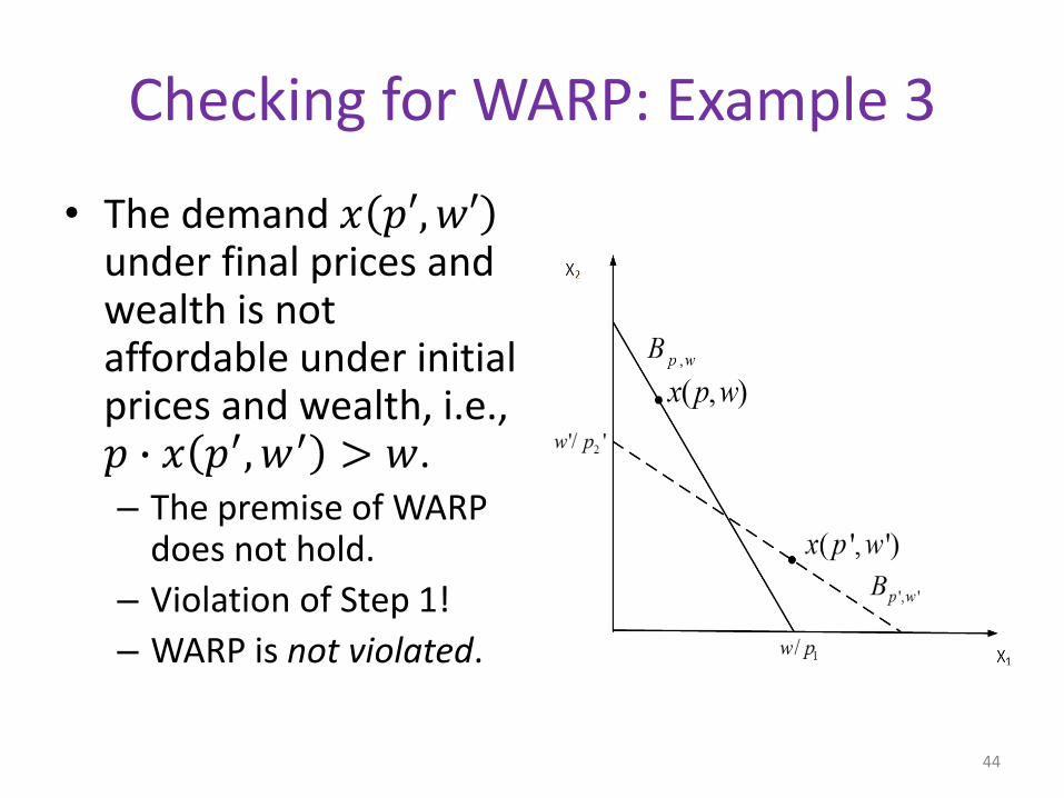
Checking for WARP: Example 3
• The demand 𝑥 𝑝′, 𝑤′under final prices and wealth is not affordable under initial prices and wealth, i.e., 𝑝 ∙ 𝑥 𝑝′, 𝑤′ > 𝑤.– The premise of WARP
does not hold.
– Violation of Step 1!
– WARP is not violated.
44

Checking for WARP: Example 4
• The demand 𝑥 𝑝′, 𝑤′under final prices and wealth is not affordable under initial prices and wealth, i.e., 𝑝 ∙ 𝑥 𝑝′, 𝑤′ > 𝑤.– The premise of WARP
does not hold.
– Violation of Step 1!
– WARP is not violated.
45

Checking for WARP: Example 5
46
x1
x2
w p2
wp1
Bp,w
Bp ,w x (p,w)x (p ,w )
• First, 𝑥 𝑝, 𝑤 and 𝑥 𝑝′, 𝑤′ are both affordable under 𝐵𝑝,𝑤.
• Second, 𝑥 𝑝, 𝑤 is affordable under 𝐵𝑝′,𝑤′, i.e., 𝑝′ ∙ 𝑥 𝑝, 𝑤 < 𝑤′
• Hence, WARP is NOTsatisfied!
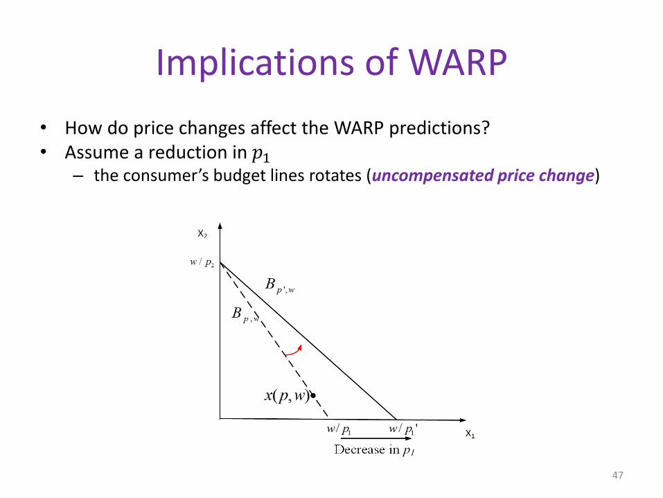
Implications of WARP
• How do price changes affect the WARP predictions?• Assume a reduction in 𝑝1
– the consumer’s budget lines rotates (uncompensated price change)
47
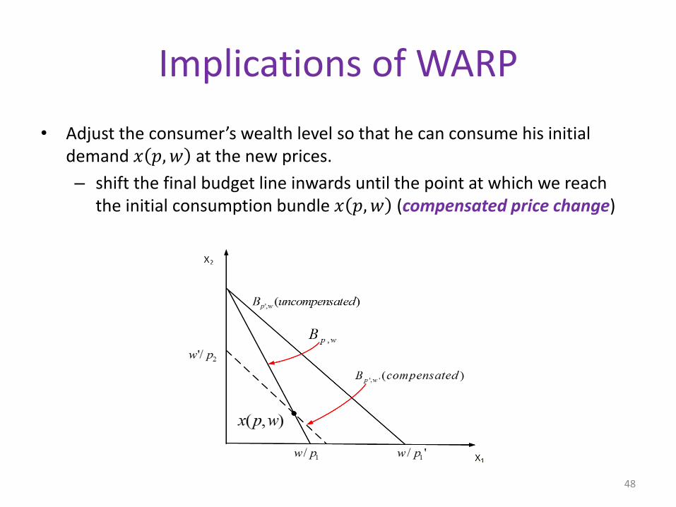
Implications of WARP
• Adjust the consumer’s wealth level so that he can consume his initial demand 𝑥 𝑝, 𝑤 at the new prices.
– shift the final budget line inwards until the point at which we reach the initial consumption bundle 𝑥 𝑝, 𝑤 (compensated price change)
48

Implications of WARP
• What is the wealth adjustment?𝑤 = 𝑝 ∙ 𝑥 𝑝, 𝑤 under 𝑝, 𝑤
𝑤′ = 𝑝′ ∙ 𝑥 𝑝, 𝑤 under 𝑝′, 𝑤′
• Then,∆𝑤 = ∆𝑝 ∙ 𝑥 𝑝, 𝑤
where ∆𝑤 = 𝑤′ − 𝑤 and ∆𝑝 = 𝑝′ − 𝑝.
• This is the Slutsky wealth compensation: – the increase (decrease) in wealth, measured by ∆𝑤, that we
must provide to the consumer so that he can afford the same consumption bundle as before the price change, i.e., 𝑥 𝑝, 𝑤 .
49
Implications of WARP: Law of Demand
• Suppose that the Walrasian demand 𝑥 𝑝, 𝑤 satisfies homog(0) and Walras’ Law. Then, 𝑥 𝑝, 𝑤 satisfies WARP iff:
∆𝑝 ∙ ∆𝑥 ≤ 0
where– ∆𝑝 = 𝑝′ − 𝑝 and ∆𝑥 = 𝑥 𝑝′, 𝑤′ − 𝑥 𝑝, 𝑤
– 𝑤′ is the wealth level that allows the consumer to buy the initial demand at the new prices, 𝑤′ = 𝑝′ ∙ 𝑥 𝑝, 𝑤
• This is the Law of Demand: quantity demanded and price move in different directions.
50
Implications of WARP: Law of Demand
• Does WARP restrict behavior when we apply Slutsky wealth compensations? – Yes!
• What if we were not applying the Slutsky wealth compensation, would WARP impose any restriction on allowable locations for 𝑥 𝑝′, 𝑤′ ?– No!
51
Implications of WARP: Law of Demand
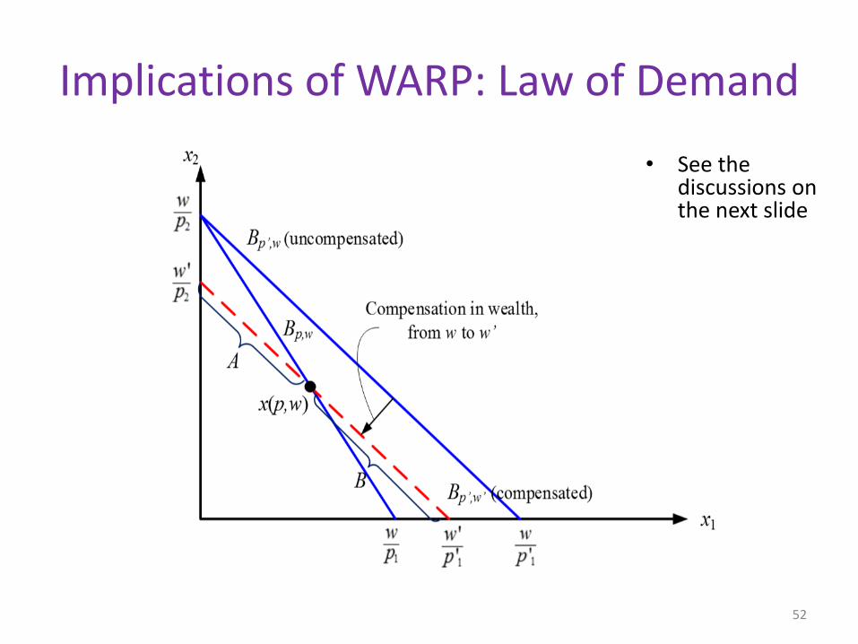
52
• See the discussions on the next slide
Implications of WARP: Law of Demand
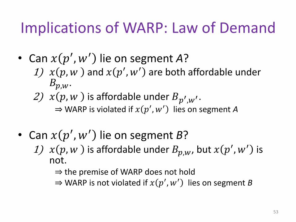
• Can 𝑥 𝑝′, 𝑤′ lie on segment A?1) 𝑥 𝑝, 𝑤 and 𝑥 𝑝′, 𝑤′ are both affordable under
𝐵𝑝,𝑤.
2) 𝑥 𝑝, 𝑤 is affordable under 𝐵𝑝′,𝑤′. ⇒ WARP is violated if 𝑥 𝑝′, 𝑤′ lies on segment A
• Can 𝑥 𝑝′, 𝑤′ lie on segment B?1) 𝑥 𝑝, 𝑤 is affordable under 𝐵𝑝,𝑤, but 𝑥 𝑝′, 𝑤′ is
not. ⇒ the premise of WARP does not hold⇒ WARP is not violated if 𝑥 𝑝′, 𝑤′ lies on segment B
53
Implications of WARP: Law of Demand
• What did we learn from this figure?1) We started from 𝛻𝑝1, and compensated the wealth of
this individual (reducing it from 𝑤 to 𝑤′) so that he could afford his initial bundle 𝑥 𝑝, 𝑤 under the new prices. From this wealth compensation, we obtained budget line 𝐵𝑝′,𝑤′.
2) From WARP, we know that 𝑥 𝑝′, 𝑤′ must contain more of good 1. That is, graphically, segment B lies to the right-hand side of
𝑥 𝑝, 𝑤 .
3) Then, a price reduction, 𝛻𝑝1, when followed by an appropriate wealth compensation leads to an increase in the quantity demanded of this good, ∆𝑥1. This is the compensated law of demand (CLD).
54
Implications of WARP: Law of Demand
• Practice problem:– Can you repeat this analysis but for an increase in
the price of good 1? First, pivot budget line 𝐵𝑝,𝑤 inwards to obtain 𝐵𝑝′,𝑤.
Then, increase the wealth level (wealth compensation) to obtain 𝐵𝑝′,𝑤′.
Identify the two segments in budget line 𝐵𝑝′,𝑤′, one to the right-hand side of 𝑥 𝑝, 𝑤 and other to the left.
In which segment of budget line 𝐵𝑝′,𝑤′ can the Walrasian demand 𝑥(𝑝′, 𝑤′) lie?
Advanced Microeconomic Theory 55
Implications of WARP: Law of Demand
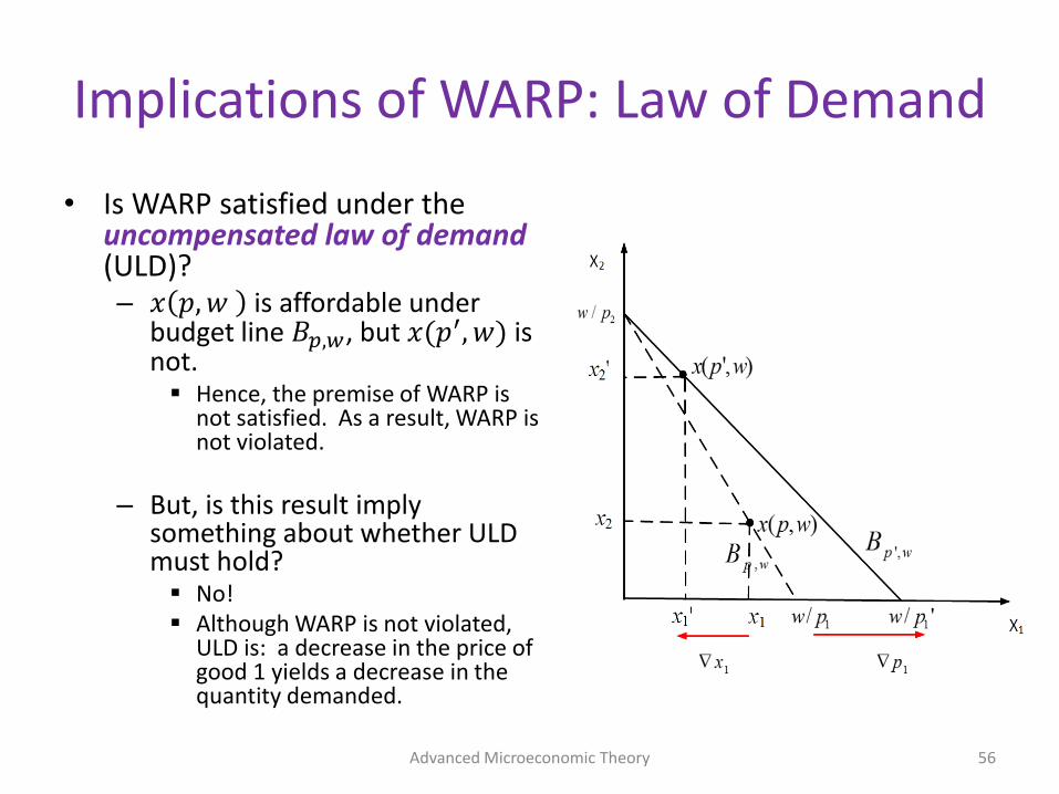
• Is WARP satisfied under the uncompensated law of demand (ULD)?– 𝑥 𝑝, 𝑤 is affordable under
budget line 𝐵𝑝,𝑤, but 𝑥(𝑝′, 𝑤) is not. Hence, the premise of WARP is
not satisfied. As a result, WARP is not violated.
– But, is this result imply something about whether ULD must hold? No! Although WARP is not violated,
ULD is: a decrease in the price of good 1 yields a decrease in the quantity demanded.
Advanced Microeconomic Theory 56

Implications of WARP: Law of Demand
• Distinction between the uncompensated and the compensated law of demand:– quantity demanded and price can move in the same
direction, when wealth is left uncompensated, i.e.,
∆𝑝1 ∙ ∆𝑥1 > 0as ∆𝑝1 ⇒ ∆𝑥1
• Hence, WARP is not sufficient to yield law of demand for price changes that are uncompensated, i.e.,
WARP ⇎ ULD, butWARP ⇔ CLD
Advanced Microeconomic Theory 57
Implications of WARP: Slutsky Matrix
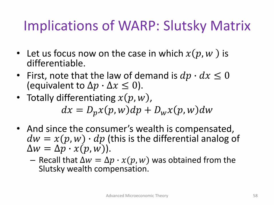
• Let us focus now on the case in which 𝑥 𝑝, 𝑤 is differentiable.
• First, note that the law of demand is 𝑑𝑝 ∙ 𝑑𝑥 ≤ 0(equivalent to ∆𝑝 ∙ ∆𝑥 ≤ 0).
• Totally differentiating 𝑥 𝑝, 𝑤 ,𝑑𝑥 = 𝐷𝑝𝑥 𝑝, 𝑤 𝑑𝑝 + 𝐷𝑤𝑥 𝑝, 𝑤 𝑑𝑤
• And since the consumer’s wealth is compensated, 𝑑𝑤 = 𝑥(𝑝, 𝑤) ∙ 𝑑𝑝 (this is the differential analog of ∆𝑤 = ∆𝑝 ∙ 𝑥(𝑝, 𝑤)).– Recall that ∆𝑤 = ∆𝑝 ∙ 𝑥(𝑝, 𝑤) was obtained from the
Slutsky wealth compensation.
Advanced Microeconomic Theory 58
Implications of WARP: Slutsky Matrix
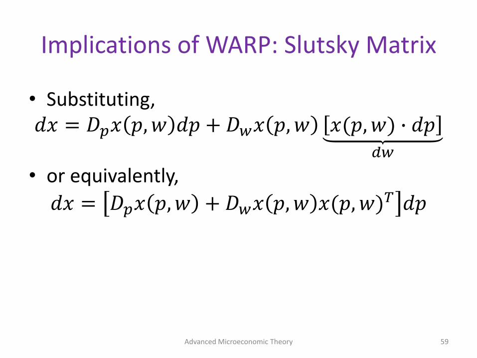
• Substituting,𝑑𝑥 = 𝐷𝑝𝑥 𝑝, 𝑤 𝑑𝑝 + 𝐷𝑤𝑥 𝑝, 𝑤 𝑥(𝑝, 𝑤) ∙ 𝑑𝑝
𝑑𝑤
• or equivalently,
𝑑𝑥 = 𝐷𝑝𝑥 𝑝, 𝑤 + 𝐷𝑤𝑥 𝑝, 𝑤 𝑥(𝑝, 𝑤)𝑇 𝑑𝑝
Advanced Microeconomic Theory 59
Implications of WARP: Slutsky Matrix
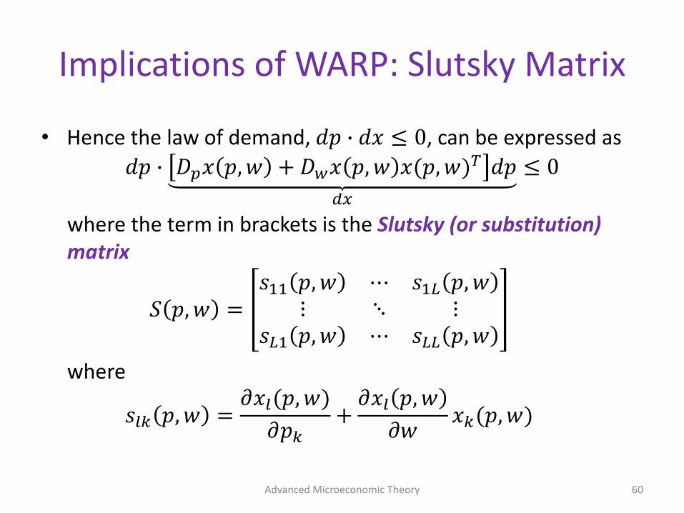
• Hence the law of demand, 𝑑𝑝 ∙ 𝑑𝑥 ≤ 0, can be expressed as
𝑑𝑝 ∙ 𝐷𝑝𝑥 𝑝, 𝑤 + 𝐷𝑤𝑥 𝑝, 𝑤 𝑥(𝑝, 𝑤)𝑇 𝑑𝑝
𝑑𝑥
≤ 0
where the term in brackets is the Slutsky (or substitution) matrix
𝑆 𝑝, 𝑤 =𝑠11 𝑝, 𝑤 ⋯ 𝑠1𝐿 𝑝, 𝑤
⋮ ⋱ ⋮𝑠𝐿1 𝑝, 𝑤 ⋯ 𝑠𝐿𝐿 𝑝, 𝑤
where
𝑠𝑙𝑘 𝑝, 𝑤 =𝜕𝑥𝑙(𝑝, 𝑤)
𝜕𝑝𝑘+
𝜕𝑥𝑙 𝑝, 𝑤
𝜕𝑤𝑥𝑘(𝑝, 𝑤)
Advanced Microeconomic Theory 60
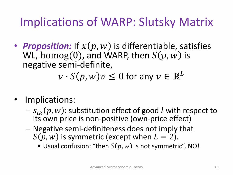
Implications of WARP: Slutsky Matrix
• Proposition: If 𝑥 𝑝, 𝑤 is differentiable, satisfies WL, homog(0), and WARP, then 𝑆 𝑝, 𝑤 is negative semi-definite,
𝑣 ∙ 𝑆 𝑝, 𝑤 𝑣 ≤ 0 for any 𝑣 ∈ ℝ𝐿
• Implications:– 𝑠𝑙𝑘 𝑝, 𝑤 : substitution effect of good 𝑙 with respect to
its own price is non-positive (own-price effect)– Negative semi-definiteness does not imply that
𝑆 𝑝, 𝑤 is symmetric (except when 𝐿 = 2). Usual confusion: “then 𝑆 𝑝, 𝑤 is not symmetric”, NO!
Advanced Microeconomic Theory 61

Implications of WARP: Slutsky Matrix
• Proposition: If preferences satisfy LNS and strict convexity, and they are represented with a continuous utility function, then the Walrasian demand 𝑥 𝑝, 𝑤generates a Slutsky matrix, 𝑆 𝑝, 𝑤 , which is symmetric.
• The above assumptions are really common. – Hence, the Slutsky matrix will then be symmetric.
• However, the above assumptions are not satisfied in the case of preferences over perfect substitutes (i.e., preferences are convex, but not strictly convex).
Advanced Microeconomic Theory 62
Implications of WARP: Slutsky Matrix
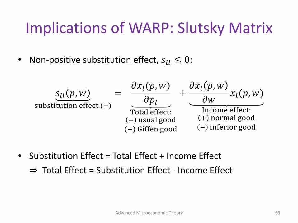
• Non-positive substitution effect, 𝑠𝑙𝑙 ≤ 0:
𝑠𝑙𝑙 𝑝, 𝑤substitution effect (−)
=𝜕𝑥𝑙(𝑝, 𝑤)
𝜕𝑝𝑙
Total effect:− usual good
+ Giffen good
+𝜕𝑥𝑙 𝑝, 𝑤
𝜕𝑤𝑥𝑙(𝑝, 𝑤)
Income effect:+ normal good
− inferior good
• Substitution Effect = Total Effect + Income Effect
⇒ Total Effect = Substitution Effect - Income Effect
Advanced Microeconomic Theory 63

Implications of WARP: Slutsky Equation
𝑠𝑙𝑙 𝑝, 𝑤substitution effect (−)
=𝜕𝑥𝑙(𝑝, 𝑤)
𝜕𝑝𝑙
Total effect
+𝜕𝑥𝑙 𝑝, 𝑤
𝜕𝑤𝑥𝑙(𝑝, 𝑤)
Income effect
• Total Effect: measures how the quantity demanded is affected by a change in the price of good 𝑙, when we leave the wealth uncompensated.
• Income Effect: measures the change in the quantity demanded as a result of the wealth adjustment.
• Substitution Effect: measures how the quantity demanded is affected by a change in the price of good 𝑙, after the wealth adjustment.– That is, the substitution effect only captures the change in demand due to variation
in the price ratio, but abstracts from the larger (smaller) purchasing power that the consumer experiences after a decrease (increase, respectively) in prices.
Advanced Microeconomic Theory 64
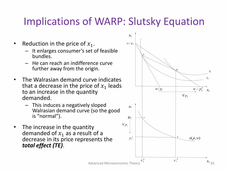
• Reduction in the price of 𝑥1. – It enlarges consumer’s set of feasible
bundles. – He can reach an indifference curve
further away from the origin.
• The Walrasian demand curve indicates that a decrease in the price of 𝑥1 leads to an increase in the quantity demanded.– This induces a negatively sloped
Walrasian demand curve (so the good is “normal”).
• The increase in the quantity demanded of 𝑥1 as a result of a decrease in its price represents the total effect (TE).
Advanced Microeconomic Theory 65
Implications of WARP: Slutsky EquationX2
X1
I2
I1
p1
X1
p1
A
B
a
b

• Reduction in the price of 𝑥1.– Disentangle the total effect into the
substitution and income effects– Slutsky wealth compensation?
• Reduce the consumer’s wealth so that he can afford the same consumption bundle as the one before the price change (i.e., A).– Shift the budget line after the price change
inwards until it “crosses” through the initial bundle A.
– “Constant purchasing power” demand curve (CPP curve) results from applying the Slutsky wealth compensation.
– The quantity demanded for 𝑥1 increases from 𝑥1
0 to 𝑥13.
• When we do not hold the consumer’s purchasing power constant, we observe relatively large increase in the quantity demanded for 𝑥1 (i.e., from 𝑥1
0 to 𝑥12 ).
Advanced Microeconomic Theory 66
Implications of WARP: Slutsky Equationx2
x1
I2
I1
p1
x1
p1
I3
CPP demand
A
B
C
a
bc

• Reduction in the price of 𝑥1.– Hicksian wealth compensation (i.e.,
“constant utility” demand curve)?
• The consumer’s wealth level is adjusted so that he can still reach his initial utility level (i.e., the same indifference curve 𝐼1as before the price change).– A more significant wealth reduction than
when we apply the Slutsky wealth compensation.
– The Hicksian demand curve reflects that, for a given decrease in p1, the consumer slightly increases his consumption of good one.
• In summary, a given decrease in 𝑝1produces: – A small increase in the Hicksian demand for
the good, i.e., from 𝑥10 to 𝑥1
1. – A larger increase in the CPP demand for the
good, i.e., from 𝑥10 to 𝑥1
3. – A substantial increase in the Walrasian
demand for the product, i.e., from 𝑥10 to 𝑥1
2.Advanced Microeconomic Theory 67
Implications of WARP: Slutsky Equationx2
x1
I2
I1
p1
x1
p1
I3
CPP demand
Hicksian demand

• A decrease in price of 𝑥1 leads the consumer to increase his consumption of this good, ∆𝑥1, but:
– The ∆𝑥1 which is solely due to the price effect (either measured by the Hicksian demand curve or the CPP demand curve) is smaller than the ∆𝑥1 measured by the Walrasian demand, 𝑥 𝑝, 𝑤 , which also captures wealth effects.
– The wealth compensation (a reduction in the consumer’s wealth in this case) that maintains the original utility level (as required by the Hicksian demand) is larger than the wealth compensation that maintains his purchasing power unaltered (as required by the Slutsky wealth compensation, in the CPP curve).
Advanced Microeconomic Theory 68
Implications of WARP: Slutsky Equation

Substitution and Income Effects: Normal Goods
• Decrease in the price of the good in the horizontal axis (i.e., food).
• The substitution effect (SE) moves in the opposite direction as the price change.
– A reduction in the price of food implies a positive substitution effect.
• The income effect (IE) is positive (thus it reinforces the SE).
– The good is normal.
Advanced Microeconomic Theory 69
Clothing
FoodSE IE
TE
A
B
C
I2
I1
BL2
BL1
BLd
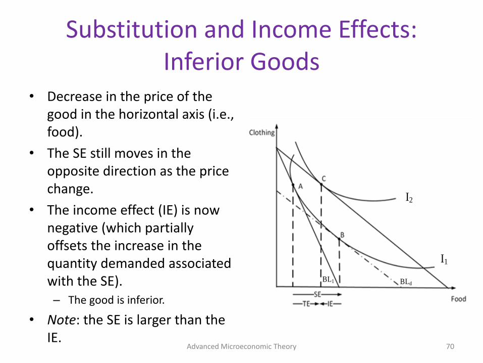
Substitution and Income Effects: Inferior Goods
• Decrease in the price of the good in the horizontal axis (i.e., food).
• The SE still moves in the opposite direction as the price change.
• The income effect (IE) is now negative (which partially offsets the increase in the quantity demanded associated with the SE). – The good is inferior.
• Note: the SE is larger than the IE.
Advanced Microeconomic Theory 70
I2
I1
BL1 BLd

Substitution and Income Effects: Giffen Goods
• Decrease in the price of the good in the horizontal axis (i.e., food).
• The SE still moves in the opposite direction as the price change.
• The income effect (IE) is still negative but now completely offsets the increase in the quantity demanded associated with the SE. – The good is Giffen good.
• Note: the SE is less than the IE.
71
I2
I1BL1
BL2
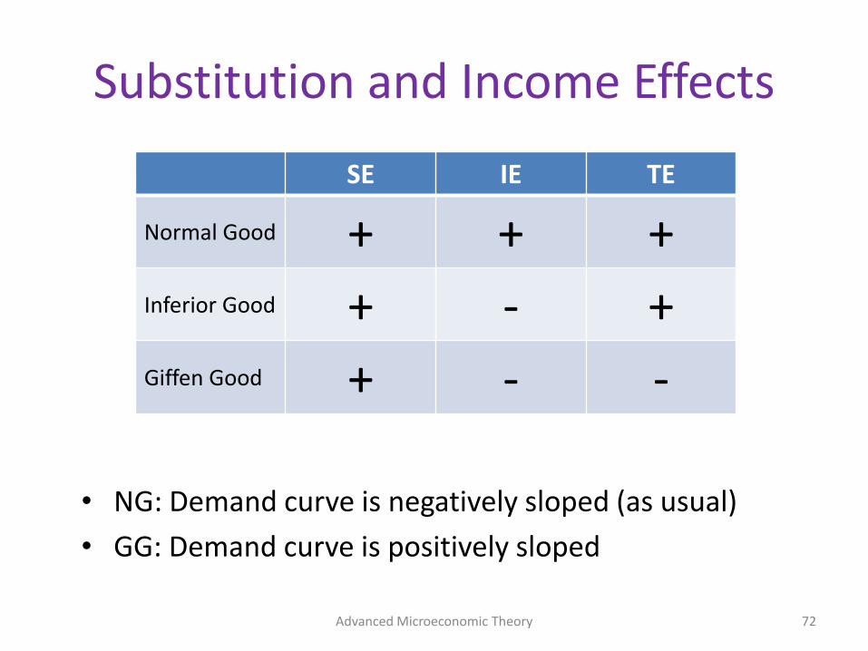
Substitution and Income Effects
SE IE TE
Normal Good + + +Inferior Good + - +Giffen Good + - -
Advanced Microeconomic Theory 72
• NG: Demand curve is negatively sloped (as usual)
• GG: Demand curve is positively sloped

Substitution and Income Effects
• Summary:1) SE is negative (since ↓ 𝑝1 ⇒ ↑ 𝑥1)
SE < 0 does not imply ↓ 𝑥1
2) If good is inferior, IE < 0. Then,
TE = ณSE− ต
− ณIE−
+
⇒ if IE><
SE , then TE(−)TE(+)
For a price decrease, this impliesTE(−)TE(+)
⇒↓ 𝑥1
↑ 𝑥1
Giffen goodNon−Giffen good
3) Hence,a) A good can be inferior, but not necessarily be Giffenb) But all Giffen goods must be inferior.
Advanced Microeconomic Theory 73

Expenditure Minimization Problem
Advanced Microeconomic Theory 74
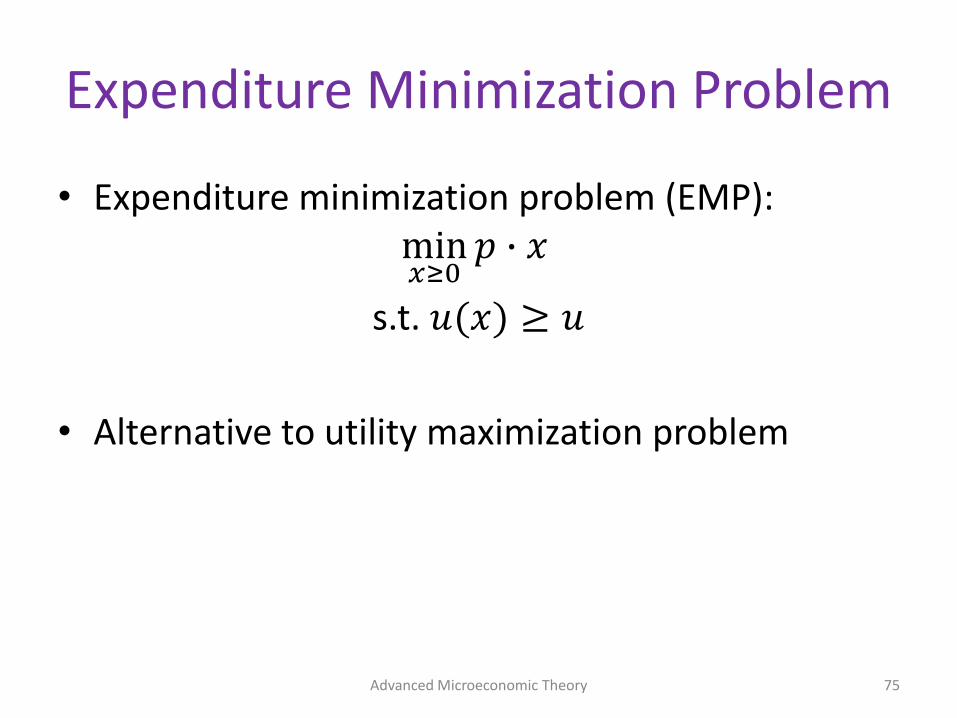
Expenditure Minimization Problem
• Expenditure minimization problem (EMP):min𝑥≥0
𝑝 ∙ 𝑥
s.t. 𝑢(𝑥) ≥ 𝑢
• Alternative to utility maximization problem
Advanced Microeconomic Theory 75

Expenditure Minimization Problem
• Consumer seeks a utility level associated with a particular indifference curve, while spending as little as possible.
• Bundles strictly above 𝑥∗ cannot be a solution to the EMP:– They reach the utility level 𝑢– But, they do not minimize total
expenditure
• Bundles on the budget line strictly below 𝑥∗ cannot be the solution to the EMP problem:– They are cheaper than 𝑥∗
– But, they do not reach the utility level 𝑢
Advanced Microeconomic Theory 76
X2
X1
*x
*UCS( )x
u

Expenditure Minimization Problem
• Lagrangian𝐿 = 𝑝 ∙ 𝑥 + 𝜇 𝑢 − 𝑢(𝑥)
• FOCs (necessary conditions)𝜕𝐿
𝜕𝑥𝑘= 𝑝𝑘 − 𝜇
𝜕𝑢(𝑥∗)
𝜕𝑥𝑘≤ 0
𝜕𝐿
𝜕𝜇= 𝑢 − 𝑢 𝑥∗ = 0
Advanced Microeconomic Theory 77
[ = 0 for interior solutions ]

Expenditure Minimization Problem
• For interior solutions,
𝑝𝑘 = 𝜇𝜕𝑢(𝑥∗)
𝜕𝑥𝑘or
1
𝜇=
𝜕𝑢(𝑥∗)
𝜕𝑥𝑘
𝑝𝑘
for any good 𝑘. This implies, 𝜕𝑢(𝑥∗)
𝜕𝑥𝑘
𝑝𝑘=
𝜕𝑢(𝑥∗)
𝜕𝑥𝑙
𝑝𝑙or
𝑝𝑘
𝑝𝑙=
𝜕𝑢(𝑥∗)
𝜕𝑥𝑘𝜕𝑢(𝑥∗)
𝜕𝑥𝑙
• The consumer allocates his consumption across goods until the point in which the marginal utility per dollar spent on each good is equal across all goods (i.e., same “bang for the buck”).
• That is, the slope of indifference curve is equal to the slope of the budget line.
Advanced Microeconomic Theory 78
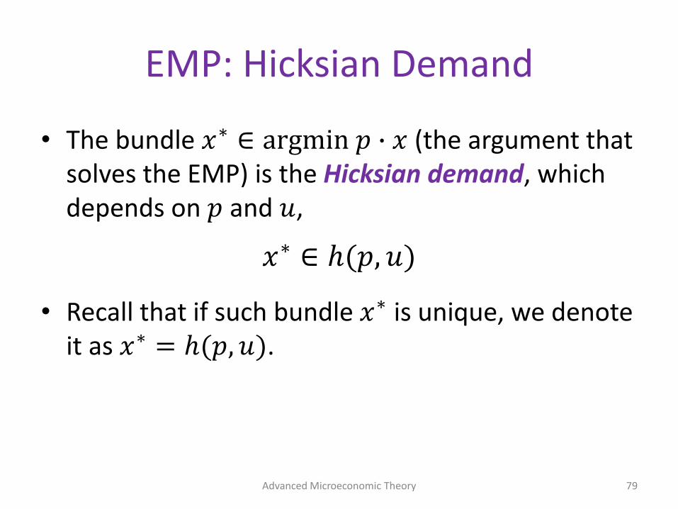
EMP: Hicksian Demand
• The bundle 𝑥∗ ∈ argmin 𝑝 ∙ 𝑥 (the argument that solves the EMP) is the Hicksian demand, which depends on 𝑝 and 𝑢,
𝑥∗ ∈ ℎ(𝑝, 𝑢)
• Recall that if such bundle 𝑥∗ is unique, we denote it as 𝑥∗ = ℎ(𝑝, 𝑢).
Advanced Microeconomic Theory 79

Properties of Hicksian Demand
• Suppose that 𝑢(∙) is a continuous function, satisfying LNS defined on 𝑋 = ℝ+
𝐿 . Then for 𝑝 ≫0, ℎ(𝑝, 𝑢) satisfies:1) Homog(0) in 𝑝, i.e., ℎ 𝑝, 𝑢 = ℎ(𝛼𝑝, 𝑢) for any 𝑝, 𝑢,
and 𝛼 > 0. If 𝑥∗ ∈ ℎ(𝑝, 𝑢) is a solution to the problem
min𝑥≥0
𝑝 ∙ 𝑥
then it is also a solution to the problemmin𝑥≥0
𝛼𝑝 ∙ 𝑥
Intuition: a common change in all prices does not alter the slope of the consumer’s budget line.
Advanced Microeconomic Theory 80

Properties of Hicksian Demand
• 𝑥∗ is a solution to the EMP when the price vector is 𝑝 = (𝑝1, 𝑝2).
• Increase all prices by factor 𝛼
𝑝′ = (𝑝1′ , 𝑝2
′ ) = (𝛼𝑝1, 𝛼𝑝2)
• Downward (parallel) shift in the budget line, i.e., the slope of the budget line is unchanged.
• But I have to reach utility level 𝑢 to satisfy the constraint of the EMP?
• Spend more to buy bundle 𝑥∗(𝑥1
∗, 𝑥2∗), i.e.,
𝑝1′ 𝑥1
∗ + 𝑝2′ 𝑥2
∗ > 𝑝1𝑥1∗ + 𝑝2𝑥2
∗
• Hence, ℎ 𝑝, 𝑢 = ℎ(𝛼𝑝, 𝑢)
Advanced Microeconomic Theory 81
x2
x1
Properties of Hicksian Demand
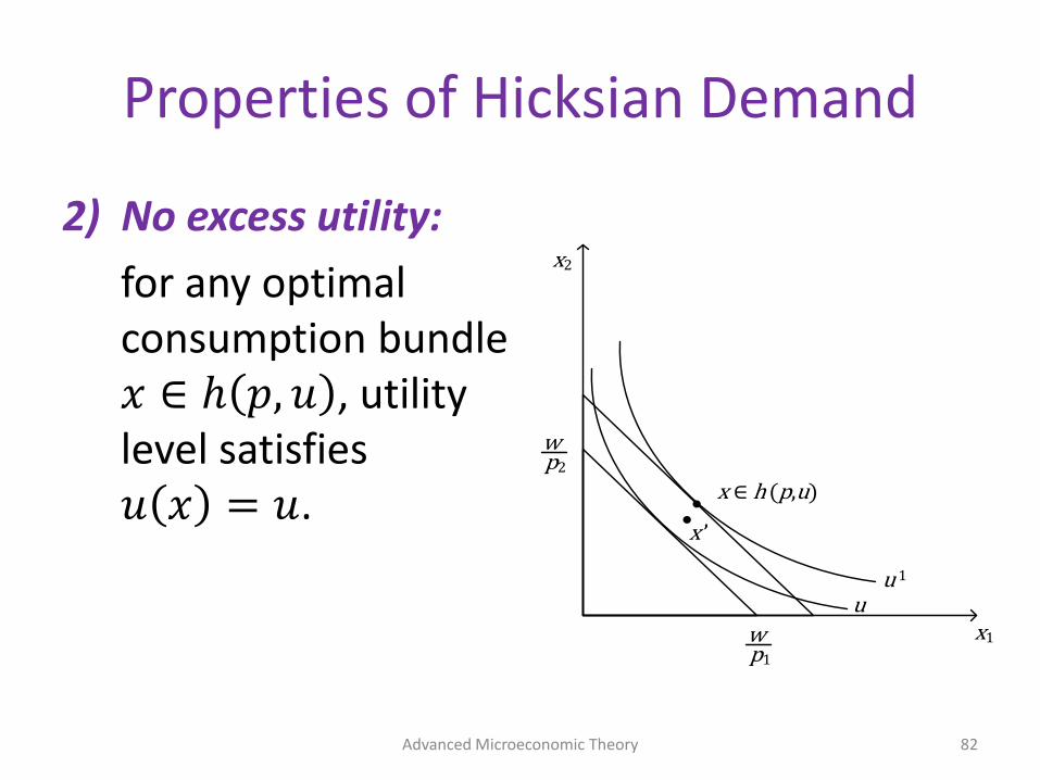
2) No excess utility:
for any optimal consumption bundle 𝑥 ∈ ℎ 𝑝, 𝑢 , utility level satisfies 𝑢 𝑥 = 𝑢.
Advanced Microeconomic Theory 82
x1
x2
wp2
wp1
x ’
x ∈ h (p,u)
uu 1
Properties of Hicksian Demand
• Intuition: Suppose there exists a bundle 𝑥 ∈ ℎ 𝑝, 𝑢 for which the consumer obtains a utility level 𝑢 𝑥 = 𝑢1 > 𝑢, which is higher than the utility level 𝑢 he must reach when solving EMP.
• But we can then find another bundle 𝑥′ = 𝑥𝛼, very close to 𝑥 (𝛼 → 1), for which 𝑢(𝑥′) > 𝑢.
• Bundle 𝑥′:– is cheaper than 𝑥– exceeds the minimal utility level 𝑢 that the consumer must
reach in his EMP
• For a given utility level 𝑢 that you have to reach in the EMP, bundle ℎ 𝑝, 𝑢 does not exceed 𝑢, since otherwise you could find a cheaper bundle that exactly reaches 𝑢.
Advanced Microeconomic Theory 83

Properties of Hicksian Demand
3) Convexity:
If the preference relation is convex, then ℎ 𝑝, 𝑢 is a convex set.
Advanced Microeconomic Theory 84
Properties of Hicksian Demand
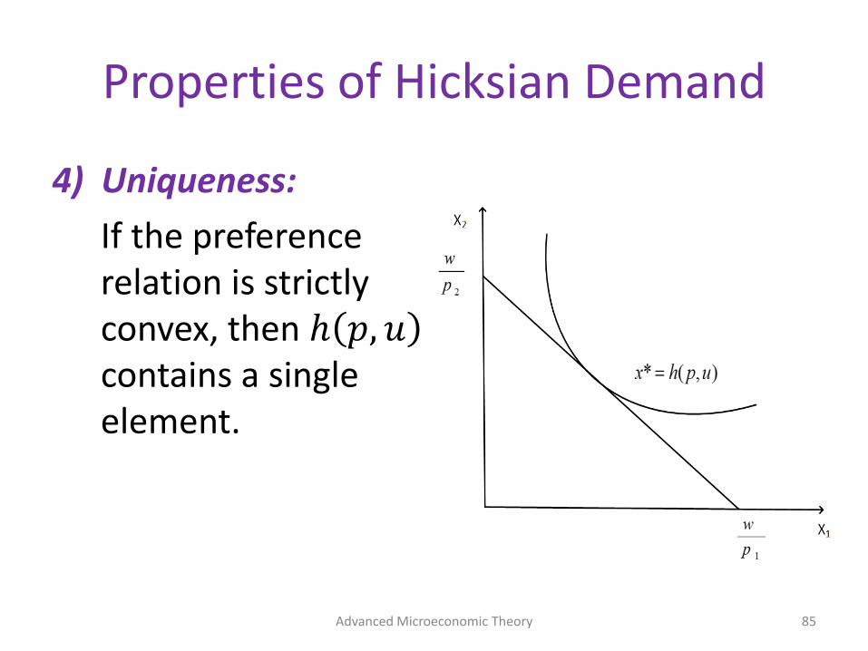
4) Uniqueness:
If the preference relation is strictly convex, then ℎ 𝑝, 𝑢contains a single element.
Advanced Microeconomic Theory 85
Properties of Hicksian Demand
• Compensated Law of Demand: for any change in prices 𝑝 and 𝑝′,
(𝑝′−𝑝) ∙ ℎ 𝑝′, 𝑢 − ℎ 𝑝, 𝑢 ≤ 0
– Implication: for every good 𝑘,(𝑝𝑘
′ − 𝑝𝑘) ∙ ℎ𝑘 𝑝′, 𝑢 − ℎ𝑘 𝑝, 𝑢 ≤ 0
– This is definitely true for compensated demand.
– But, not necessarily for Walrasian demand (which is uncompensated):
• Recall the figures on Giffen goods, where a decrease in 𝑝𝑘 in fact decreases 𝑥𝑘 𝑝, 𝑢 when wealth was uncompensated.
Advanced Microeconomic Theory 86
The Expenditure Function
• Plugging the result from the EMP, ℎ 𝑝, 𝑢 , into the objective function, 𝑝 ∙ 𝑥, we obtain the value function of this optimization problem,
𝑝 ∙ ℎ 𝑝, 𝑢 = 𝑒(𝑝, 𝑢)
where 𝑒(𝑝, 𝑢) represents the minimal expenditure that the consumer needs to incur in order to reach utility level 𝑢 when prices are 𝑝.
Advanced Microeconomic Theory 87
Properties of Expenditure Function
• Suppose that 𝑢(∙) is a continuous function, satisfying LNS defined on 𝑋 = ℝ+
𝐿 . Then for 𝑝 ≫0, 𝑒(𝑝, 𝑢) satisfies:1) Homog(1) in 𝑝, i.e.,
𝑒 𝛼𝑝, 𝑢 = 𝛼 𝑝 ∙ 𝑥∗
𝑒(𝑝,𝑢)
= 𝛼 ∙ 𝑒(𝑝, 𝑢)
for any 𝑝, 𝑢, and 𝛼 > 0.
We know that the optimal bundle is not changed when all prices change, since the optimal consumption bundle in ℎ(𝑝, 𝑢) satisfies homogeneity of degree zero.
Such change just makes it more or less expensive to buy the same bundle.
Advanced Microeconomic Theory 88
Properties of Expenditure Function
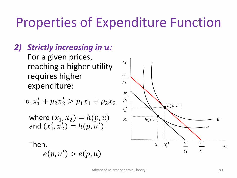
2) Strictly increasing in 𝒖: For a given prices, reaching a higher utility requires higher expenditure:
𝑝1𝑥1′ + 𝑝2𝑥2
′ > 𝑝1𝑥1 + 𝑝2𝑥2
where (𝑥1, 𝑥2) = ℎ(𝑝, 𝑢)and (𝑥1
′ , 𝑥2′ ) = ℎ(𝑝, 𝑢′).
Then,𝑒 𝑝, 𝑢′ > 𝑒 𝑝, 𝑢
Advanced Microeconomic Theory 89
x2
x1
x2
x1
Properties of Expenditure Function
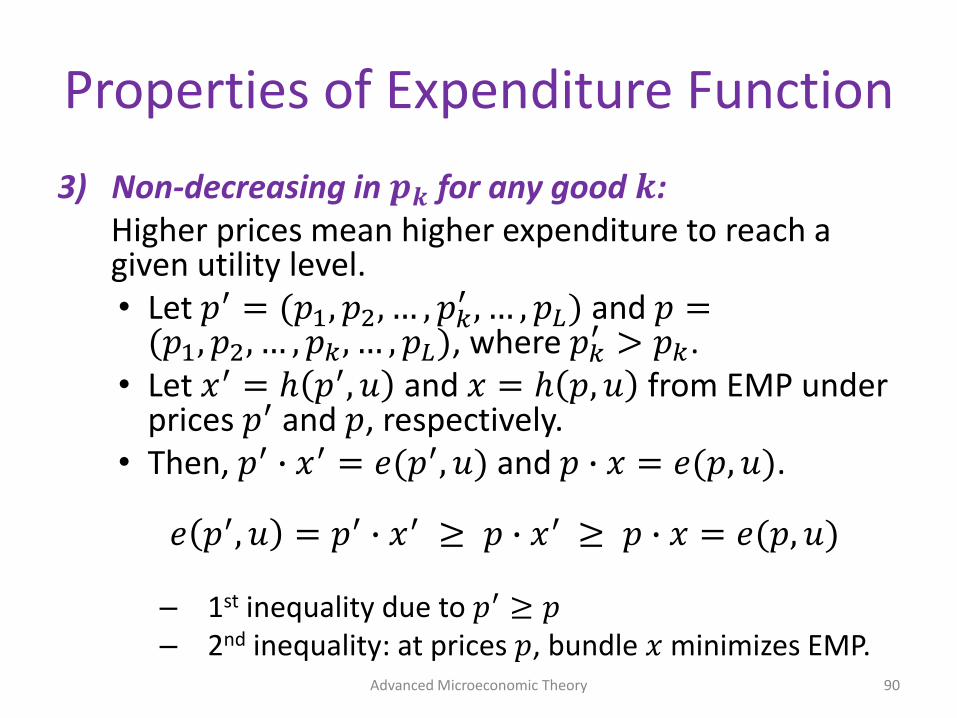
3) Non-decreasing in 𝒑𝒌 for any good 𝒌:Higher prices mean higher expenditure to reach a given utility level. • Let 𝑝′ = (𝑝1, 𝑝2, … , 𝑝𝑘
′ , … , 𝑝𝐿) and 𝑝 =(𝑝1, 𝑝2, … , 𝑝𝑘, … , 𝑝𝐿), where 𝑝𝑘
′ > 𝑝𝑘.• Let 𝑥′ = ℎ 𝑝′, 𝑢 and 𝑥 = ℎ 𝑝, 𝑢 from EMP under
prices 𝑝′ and 𝑝, respectively.• Then, 𝑝′ ∙ 𝑥′ = 𝑒(𝑝′, 𝑢) and 𝑝 ∙ 𝑥 = 𝑒(𝑝, 𝑢).
𝑒 𝑝′, 𝑢 = 𝑝′ ∙ 𝑥′ ≥ 𝑝 ∙ 𝑥′ ≥ 𝑝 ∙ 𝑥 = 𝑒(𝑝, 𝑢)
– 1st inequality due to 𝑝′ ≥ 𝑝– 2nd inequality: at prices 𝑝, bundle 𝑥 minimizes EMP.
Advanced Microeconomic Theory 90
Properties of Expenditure Function
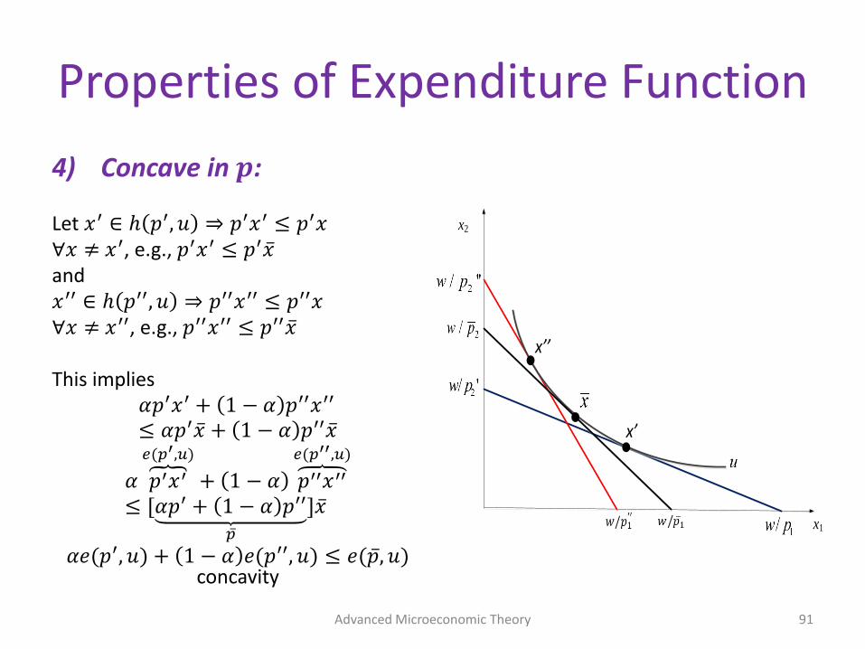
4) Concave in 𝒑:
Let 𝑥′ ∈ ℎ 𝑝′, 𝑢 ⇒ 𝑝′𝑥′ ≤ 𝑝′𝑥∀𝑥 ≠ 𝑥′, e.g., 𝑝′𝑥′ ≤ 𝑝′ ҧ𝑥and 𝑥′′ ∈ ℎ 𝑝′′, 𝑢 ⇒ 𝑝′′𝑥′′ ≤ 𝑝′′𝑥∀𝑥 ≠ 𝑥′′, e.g., 𝑝′′𝑥′′ ≤ 𝑝′′ ҧ𝑥
This implies𝛼𝑝′𝑥′ + 1 − 𝛼 𝑝′′𝑥′′
≤ 𝛼𝑝′ ҧ𝑥 + 1 − 𝛼 𝑝′′ ҧ𝑥
𝛼 ฑ𝑝′𝑥′
𝑒(𝑝′,𝑢)
+ 1 − 𝛼 𝑝′′𝑥′′
𝑒(𝑝′′,𝑢)
≤ [𝛼𝑝′ + 1 − 𝛼 𝑝′′
ҧ𝑝
] ҧ𝑥
𝛼𝑒(𝑝′, 𝑢) + 1 − 𝛼 𝑒(𝑝′′, 𝑢) ≤ 𝑒( ҧ𝑝, 𝑢)concavity
Advanced Microeconomic Theory 91
x2
x1
x
x

Connections
Advanced Microeconomic Theory 92
Relationship between the Expenditure and Hicksian Demand
• Let’s assume that 𝑢(∙) is a continuous function, representing preferences that satisfy LNS and are strictly convex and defined on 𝑋 = ℝ+
𝐿 . For all 𝑝 and 𝑢,
𝜕𝑒 𝑝,𝑢
𝜕𝑝𝑘= ℎ𝑘 𝑝, 𝑢 for every good 𝑘
This identity is “Shepard’s lemma”: if we want to find ℎ𝑘 𝑝, 𝑢 and we know 𝑒 𝑝, 𝑢 , we just have to differentiate 𝑒 𝑝, 𝑢 with respect to prices.
• Proof: three different approaches1) the support function2) first-order conditions 3) the envelop theorem (See Appendix 2.2)
Advanced Microeconomic Theory 93
Relationship between the Expenditure and Hicksian Demand
• The relationship between the Hicksian demand and the expenditure function can be further developed by taking first order conditions again. That is,
𝜕2𝑒(𝑝, 𝑢)
𝜕𝑝𝑘2 =
𝜕ℎ𝑘(𝑝, 𝑢)
𝜕𝑝𝑘
or𝐷𝑝
2𝑒 𝑝, 𝑢 = 𝐷𝑝ℎ(𝑝, 𝑢)
• Since 𝐷𝑝ℎ(𝑝, 𝑢) provides the Slutsky matrix, 𝑆(𝑝, 𝑤), then
𝑆 𝑝, 𝑤 = 𝐷𝑝2𝑒 𝑝, 𝑢
where the Slutsky matrix can be obtained from the observable Walrasian demand.
Advanced Microeconomic Theory 94

Relationship between the Expenditure and Hicksian Demand
• There are three other important properties of 𝐷𝑝ℎ(𝑝, 𝑢), where 𝐷𝑝ℎ(𝑝, 𝑢) is 𝐿 × 𝐿 derivative matrix of the hicksian demand, ℎ 𝑝, 𝑢 :1) 𝐷𝑝ℎ(𝑝, 𝑢) is negative semidefinite
Hence, 𝑆 𝑝, 𝑤 is negative semidefinite.
2) 𝐷𝑝ℎ(𝑝, 𝑢) is a symmetric matrix Hence, 𝑆 𝑝, 𝑤 is symmetric.
3) 𝐷𝑝ℎ 𝑝, 𝑢 𝑝 = 0, which implies 𝑆 𝑝, 𝑤 𝑝 = 0.
Not all goods can be net substitutes 𝜕ℎ𝑙(𝑝,𝑢)
𝜕𝑝𝑘> 0 or net
complements 𝜕ℎ𝑙(𝑝,𝑢)
𝜕𝑝𝑘< 0 . Otherwise, the multiplication
of this vector of derivatives times the (positive) price vector 𝑝 ≫ 0 would yield a non-zero result.
Advanced Microeconomic Theory 95
Relationship between Hicksian and Walrasian Demand
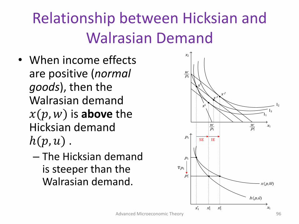
• When income effects are positive (normal goods), then the Walrasian demand 𝑥(𝑝, 𝑤) is above the Hicksian demand ℎ(𝑝, 𝑢) .– The Hicksian demand
is steeper than the Walrasian demand.
Advanced Microeconomic Theory 96
x1
x2
wp2
wp1
x1
p1
wp1
p1
p1
x*1 x1
1 x21
h (p,ū)
x (p,w)
p1
I1
I3
I2x1
x 3x 2
x*
SE IE
Relationship between Hicksian and Walrasian Demand
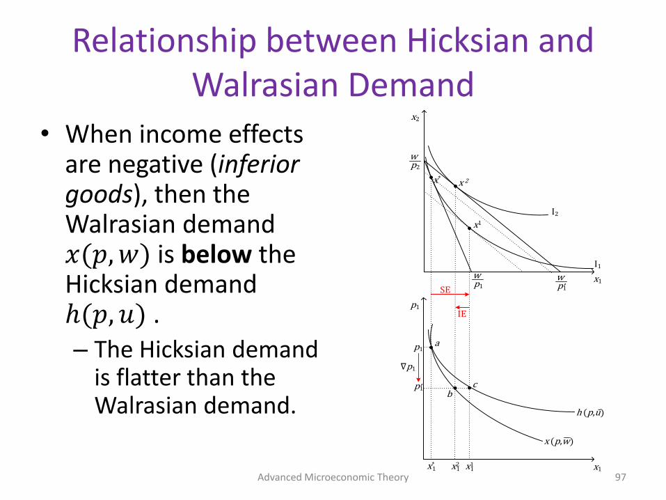
• When income effects are negative (inferior goods), then the Walrasian demand 𝑥(𝑝, 𝑤) is below the Hicksian demand ℎ(𝑝, 𝑢) .– The Hicksian demand
is flatter than the Walrasian demand.
Advanced Microeconomic Theory 97
x1
x2
wp2
wp1
x1
p1
wp1
p1
p1
x*1 x1
1x21
h (p,ū)
x (p,w)
p1
I1
I2
x1
x 2x*
SE
IE
a
bc
Relationship between Hicksian and Walrasian Demand
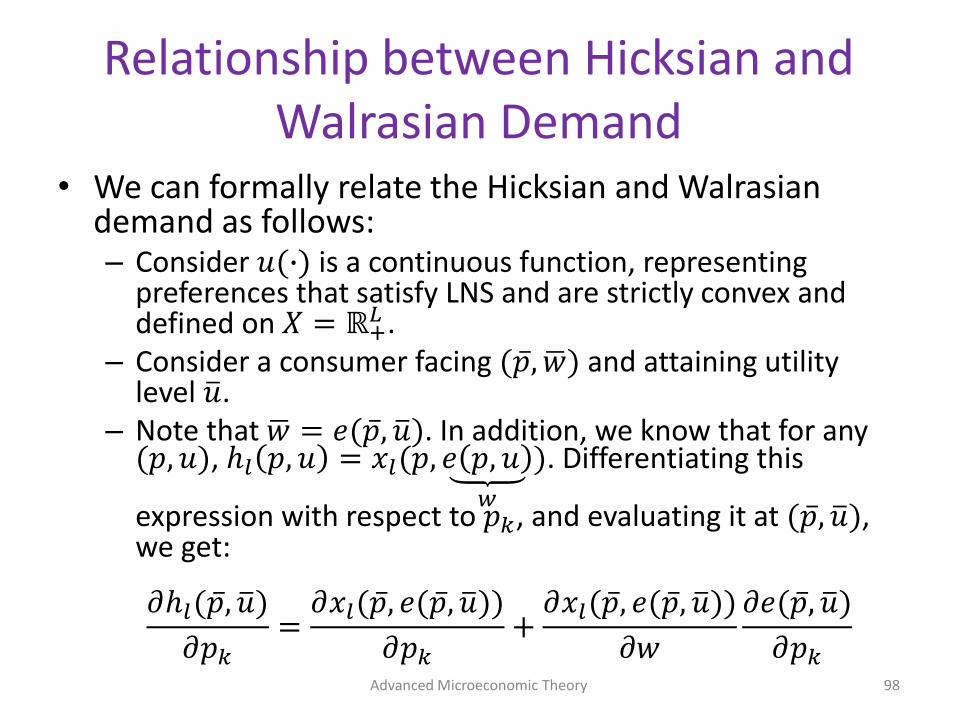
• We can formally relate the Hicksian and Walrasian demand as follows:– Consider 𝑢(∙) is a continuous function, representing
preferences that satisfy LNS and are strictly convex and defined on 𝑋 = ℝ+
𝐿 .– Consider a consumer facing ( ҧ𝑝, ഥ𝑤) and attaining utility
level ത𝑢.– Note that ഥ𝑤 = 𝑒( ҧ𝑝, ത𝑢). In addition, we know that for any
(𝑝, 𝑢), ℎ𝑙 𝑝, 𝑢 = 𝑥𝑙(𝑝, 𝑒 𝑝, 𝑢𝑤
). Differentiating this
expression with respect to 𝑝𝑘, and evaluating it at ( ҧ𝑝, ത𝑢), we get:
𝜕ℎ𝑙( ҧ𝑝, ത𝑢)
𝜕𝑝𝑘=
𝜕𝑥𝑙( ҧ𝑝, 𝑒( ҧ𝑝, ത𝑢))
𝜕𝑝𝑘+
𝜕𝑥𝑙( ҧ𝑝, 𝑒( ҧ𝑝, ത𝑢))
𝜕𝑤
𝜕𝑒( ҧ𝑝, ത𝑢)
𝜕𝑝𝑘Advanced Microeconomic Theory 98
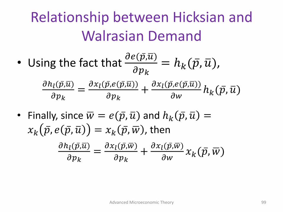
Relationship between Hicksian and Walrasian Demand
• Using the fact that 𝜕𝑒( ҧ𝑝,ഥ𝑢)
𝜕𝑝𝑘= ℎ𝑘( ҧ𝑝, ത𝑢),
𝜕ℎ𝑙( ҧ𝑝,ഥ𝑢)
𝜕𝑝𝑘=
𝜕𝑥𝑙( ҧ𝑝,𝑒( ҧ𝑝,ഥ𝑢))
𝜕𝑝𝑘+
𝜕𝑥𝑙( ҧ𝑝,𝑒( ҧ𝑝,ഥ𝑢))
𝜕𝑤ℎ𝑘( ҧ𝑝, ത𝑢)
• Finally, since ഥ𝑤 = 𝑒( ҧ𝑝, ത𝑢) and ℎ𝑘 ҧ𝑝, ത𝑢 =
𝑥𝑘 ҧ𝑝, 𝑒 ҧ𝑝, ത𝑢 = 𝑥𝑘 ҧ𝑝, ഥ𝑤 , then
𝜕ℎ𝑙( ҧ𝑝,ഥ𝑢)
𝜕𝑝𝑘=
𝜕𝑥𝑙( ҧ𝑝, ഥ𝑤)
𝜕𝑝𝑘+
𝜕𝑥𝑙( ҧ𝑝, ഥ𝑤)
𝜕𝑤𝑥𝑘( ҧ𝑝, ഥ𝑤)
Advanced Microeconomic Theory 99
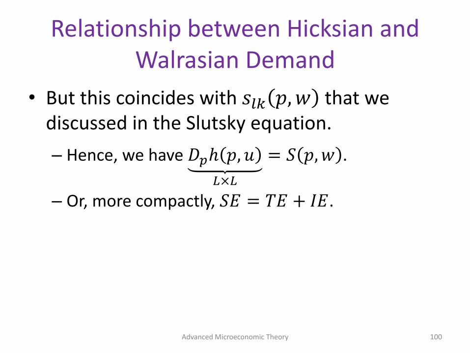
Relationship between Hicksian and Walrasian Demand
• But this coincides with 𝑠𝑙𝑘 𝑝, 𝑤 that we discussed in the Slutsky equation.
– Hence, we have 𝐷𝑝ℎ 𝑝, 𝑢
𝐿×𝐿
= 𝑆 𝑝, 𝑤 .
– Or, more compactly, 𝑆𝐸 = 𝑇𝐸 + 𝐼𝐸.
Advanced Microeconomic Theory 100
Relationship between Walrasian Demand and Indirect Utility Function
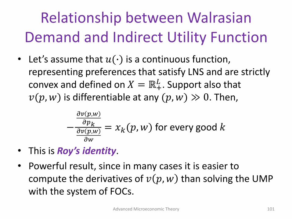
• Let’s assume that 𝑢(∙) is a continuous function, representing preferences that satisfy LNS and are strictly convex and defined on 𝑋 = ℝ+
𝐿 . Support also that 𝑣(𝑝, 𝑤) is differentiable at any (𝑝, 𝑤) ≫ 0. Then,
−
𝜕𝑣 𝑝,𝑤
𝜕𝑝𝑘𝜕𝑣 𝑝,𝑤
𝜕𝑤
= 𝑥𝑘(𝑝, 𝑤) for every good 𝑘
• This is Roy’s identity.
• Powerful result, since in many cases it is easier to compute the derivatives of 𝑣 𝑝, 𝑤 than solving the UMP with the system of FOCs.
Advanced Microeconomic Theory 101
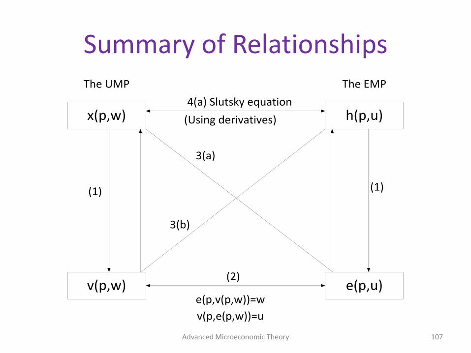
Summary of Relationships
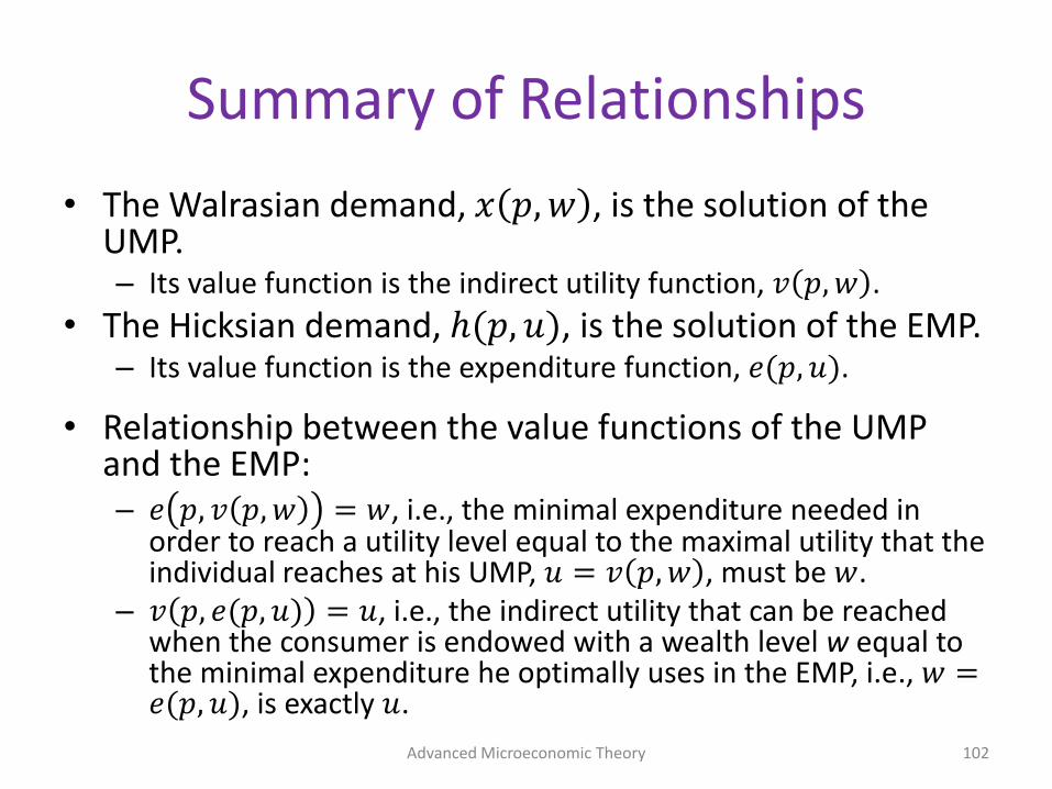
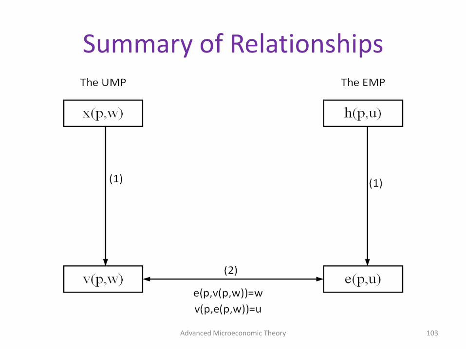
• The Walrasian demand, 𝑥 𝑝, 𝑤 , is the solution of the UMP.– Its value function is the indirect utility function, 𝑣 𝑝, 𝑤 .
• The Hicksian demand, ℎ(𝑝, 𝑢), is the solution of the EMP. – Its value function is the expenditure function, 𝑒(𝑝, 𝑢).
• Relationship between the value functions of the UMP and the EMP:– 𝑒 𝑝, 𝑣 𝑝, 𝑤 = 𝑤, i.e., the minimal expenditure needed in
order to reach a utility level equal to the maximal utility that the individual reaches at his UMP, 𝑢 = 𝑣 𝑝, 𝑤 , must be 𝑤.
– 𝑣 𝑝, 𝑒(𝑝, 𝑢) = 𝑢, i.e., the indirect utility that can be reached when the consumer is endowed with a wealth level w equal to the minimal expenditure he optimally uses in the EMP, i.e., 𝑤 =𝑒(𝑝, 𝑢), is exactly 𝑢.
Advanced Microeconomic Theory 102
Summary of Relationships
Advanced Microeconomic Theory 103

Summary of Relationships
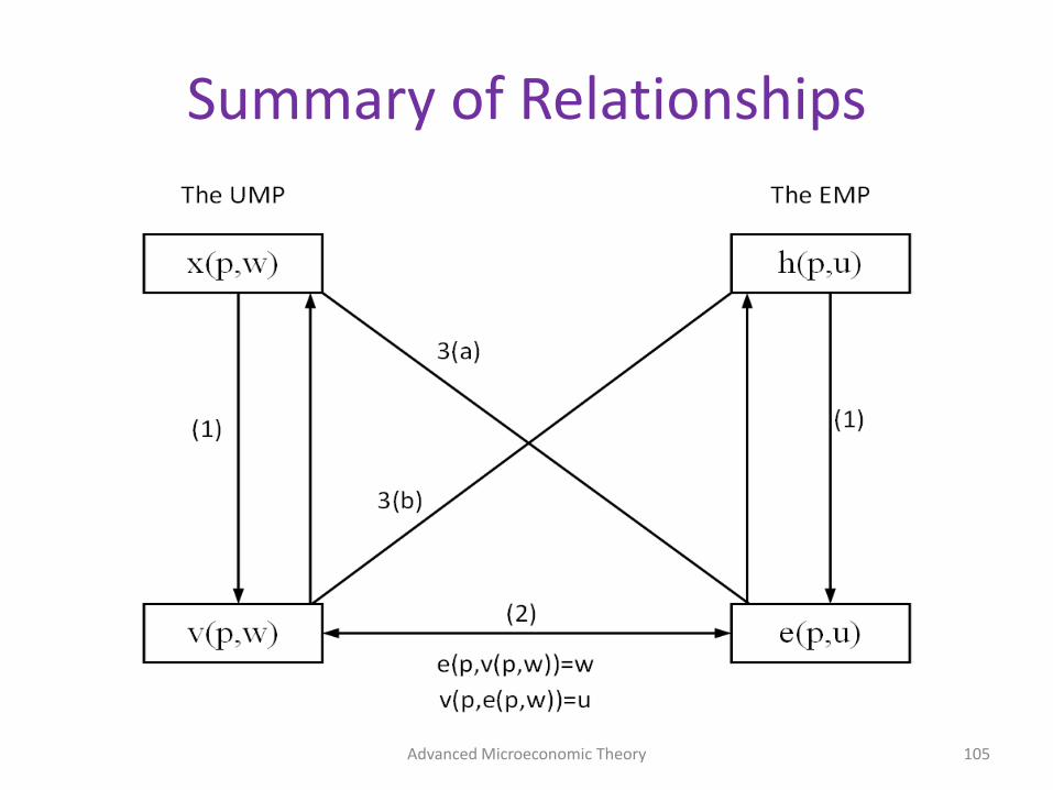
• Relationship between the argmax of the UMP (the Walrasian demand) and the argmin of the EMP (the Hicksian demand):– 𝑥 𝑝, 𝑒(𝑝, 𝑢) = ℎ 𝑝, 𝑢 , i.e., the (uncompensated)
Walrasian demand of a consumer endowed with an adjusted wealth level 𝑤 (equal to the expenditure he optimally uses in the EMP), 𝑤 = 𝑒 𝑝, 𝑢 , coincides with his Hicksian demand, ℎ 𝑝, 𝑢 .
– ℎ 𝑝, 𝑣(𝑝, 𝑤) = 𝑥 𝑝, 𝑤 , i.e., the (compensated) Hicksian demand of a consumer reaching the maximum utility of the UMP, 𝑢 = 𝑣 (𝑝, 𝑤), coincides with his Walrasian demand, 𝑥 𝑝, 𝑤 .
Advanced Microeconomic Theory 104
Summary of Relationships
Advanced Microeconomic Theory 105

Summary of Relationships
• Finally, we can also use:– The Slutsky equation:
𝜕ℎ𝑙(𝑝, 𝑢)
𝜕𝑝𝑘=
𝜕𝑥𝑙(𝑝, 𝑤)
𝜕𝑝𝑘+
𝜕𝑥𝑙(𝑝, 𝑤)
𝜕𝑤𝑥𝑘(𝑝, 𝑤)
to relate the derivatives of the Hicksian and the Walrasian demand.– Shepard’s lemma:
𝜕𝑒 𝑝, 𝑢
𝜕𝑝𝑘= ℎ𝑘 𝑝, 𝑢
to obtain the Hicksian demand from the expenditure function.– Roy’s identity:
−
𝜕𝑣 𝑝, 𝑤𝜕𝑝𝑘
𝜕𝑣 𝑝, 𝑤𝜕𝑤
= 𝑥𝑘(𝑝, 𝑤)
to obtain the Walrasian demand from the indirect utility function.
Advanced Microeconomic Theory 106
Summary of Relationships
Advanced Microeconomic Theory 107
x(p,w)
v(p,w) e(p,u)
h(p,u)
The UMP The EMP
e(p,v(p,w))=w
v(p,e(p,w))=u
(1) (1)
(2)
3(a)
3(b)
4(a) Slutsky equation
(Using derivatives)
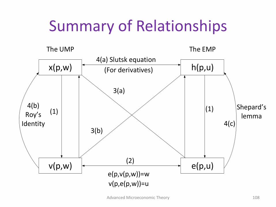
Summary of Relationships
Advanced Microeconomic Theory 108
x(p,w)
v(p,w) e(p,u)
h(p,u)
The UMP The EMP
e(p,v(p,w))=w
v(p,e(p,w))=u
(1) (1)
(2)
3(a)
3(b)
4(a) Slutsk equation
(For derivatives)
4(b) Roy s
Identity 4(c)
Shepard s lemma