chapter 2 a multi-stranded chronology of analogue computing

Chapter 2A Multi-Stranded Chronology of AnalogueComputing

This chapter describes the origins and evolution of analogue computing.1 However,it is important to emphasise that the history of modern analogue computing is in-extricably linked with the history of modern digital computing. In fact, the phrase‘analogue computing’ was only coined as a result of the invention of digital com-puters in the 1940s. In terms of the wider history of computing, the 1940s was aperiod of significant innovation and saw the unveiling of Howard Aiken’s HarvardMark I; the invention of an automatic electrical calculator by John Vincent Atana-soff; and the development of the electronic ENIAC.2 Scientific culture was thirstyfor the electronic mechanisation of mathematics, and it was from this inventive soupthat, inspired by a need to contrast the old with the new, the technical labels of ‘ana-logue’ and ‘digital’ first emerged.

The first use of the word ‘analogue’ to describe a class of computer is attributedto Atanasoff, who, although a pioneer of digital technology, had previously usedanalogue methods (before they were so-called) for solving partial differential equa-tions.3 With a new classification scheme at hand, practitioners very quickly began toapply the labels ‘analogue’ and ‘digital’ to a whole range of problem solving tech-nologies, enrolling them into a computing culture. Some of these technologies werealready considered calculating machines, but for a number of technologies and ap-

1This chapter is an expanded form of a previously published article (Care 2007a).2Developed during wartime USA, the Harvard Mark I became operational in 1944 and was basedon electro-mechanical components. However, the future for both analogue and digital computerswould be found in the speed and flexibility of electrical and electronic components. Other importantearly work includes that of the German pioneer Konrad Zuse, and engineers within the British codebreaking effort of World War II. In terms of future influence on computing technology, much ofthe significant innovation was American.3Working at Iowa State College during the 1930s, Atanasoff had developed the Laplaciometer tohelp him solve problems based on Laplace’s equations. It was therefore a tool for solving partialdifferential equations (Murphy and Atanasoff 1949).

C. Care, Technology for Modelling, History of Computing,DOI 10.1007/978-1-84882-948-0_2, © Springer-Verlag London Limited 2010

17

http://dx.doi.org/10.1007/978-1-84882-948-0_2

18 2 A Multi-Stranded Chronology of Analogue Computing

proaches, it was only through association with analogue computing that they wouldbecome ‘computational’.4

This chapter presents a chronology of analogue computing in which a distinctionis drawn between two major strands of analogue computer: one supporting calcula-tion, the other concerned with modelling. These two strands roughly correspond to aclassification established by the technology’s practitioners: namely, that of indirectand direct analogue computers. We will return to the indirect/direct distinction laterin the chapter, but for now it is enough to acknowledge that the sheer existence ofthis classification justifies approaching the history from both themes. This chapterargues that it was not until the concept of an ‘analogue computer’ emerged that thesetwo strands of the technology’s history were unified (to form a third strand).5

2.1 Two Meanings of Analogue: The Tension Between Analogyand Continuity

Before we begin, it is important to clarify some terminology. In English, the wordanalogue has traditionally been used to convey likeness, similarity or correspon-dence. Like analogy, it derives from the Greek analogon for equalities of ratio orproportion.6 During the twentieth century, the word developed a second technicalmeaning: one now commonly employed to describe electromagnetic waveforms.Rather than a discrete or digital signal, an analogue waveform is a continuous func-tion (see Fig. 2.1). It is from this second meaning that the technical labels ‘analoguetelevision’ and ‘analogue radio’ are derived, and as a result of this technical use,‘analogue’ is now used to refer to continuity in general. For instance, popular usageof the analogue–digital dichotomy is found in the classification of clocks—analogueclocks employ a continuous representation of time (the rotation of the clock’s hands)

4The survey of calculating machines by Vannevar Bush in his Gibbs lecture (Bush 1936) and Ir-ven Travis’ Moore School lecture (Travis 1946) indicate how the early technology was perceived.Travis also produced an extensive bibliography (Travis 1938) which nicely preserves his perspec-tive on the scope of relevant technology. In this work, Travis makes no reference to network anal-ysers or other physical models.5As Akera (2007) writes: ‘Before World War II, computing was not yet a unified field; it wasa loose agglomeration of local practices sustained through various institutional niches for com-mercial accounting, scientific computing, and engineering analysis’ (p. 25). We will see how thetechnologies that came to be known as analogue were a unification of both calculating and analysistools.6This ‘similarity’ is understood to be structural, concerning correspondences of formrather than content. See ‘Analogue, n., and a.’, The Oxford English Dictionary,2nd edn. 1989. OED online 2010, Oxford University Press, Accessed Feb. 2010,http://dictionary.oed.com/cgi/entry/50007887; ‘analogon’, The Oxford English Dictio-nary, 2nd edn. 1989. OED online 2010, Oxford University Press, Accessed Feb. 2010,http://dictionary.oed.com/cgi/entry/50007883; and ‘analogy’, The Oxford English Dictio-nary, 2nd edn. 1989. OED online 2010, Oxford University Press, Accessed Feb. 2010,http://dictionary.oed.com/cgi/entry/50007888.

http://dictionary.oed.com/cgi/entry/50007887



2.1 Two Meanings of Analogue: The Tension Between Analogy and Continuity 19

Fig. 2.1 An example of an analogue and digital signal varying over time. The signal on the leftvaries over a continuous range to the granularity imposed by physical properties. The signal onthe right has been digitalised over a range of discrete values. Alongside analogy, continuity is asecond meaning of analogue. Note that this example only demonstrates digitalisation of the signal’smagnitude (or range), waveforms can also be discrete or continuous with respect to time

whereas digital ones use numeric digits. Additionally, recent advances in digital au-dio have resulted in digital acting as a key word for sound reproduction: analoguerepresenting the crackly, out-moded, and less desirable technologies of vinyl recordsand tape cassettes.7

If the word analogue has two meanings, analogue computing can be understoodin terms of them both. Firstly, analogue computers rely on the construction of asuitable analogy (or correspondence) between two physical systems; secondly, ana-logue computers use an internal representation that is continuous.8 That analoguecomputing can be interpreted through both meanings is not simply a convenientcoincidence. Certain analogue computers were originally referred to as ‘analogymachines’ and the association of the word with continuity arose through the com-parison of these machines with their competitor technology, the digital computer.The double meaning exists as a direct result of analogue computing.

Shaped by usage, the word ‘analogue’ evolved to become synonymous with con-tinuity, establishing a term that was subsequently exported to other technical cul-tures such as signal processing and control engineering. In turn, analogue becamea technical label in the consumer culture of audio and video technologies. It couldbe argued that this is the most significant cultural legacy of analogue computing.

7Many examples of shifting contexts and the ‘overloading’ of technical labels exist. One exampleis ‘personal stereo’, the technical term for two-channel audio—stereo—becoming synonymouswith a product. Similarly the musical term for soft dynamics (piano) has become a label for theinstrument that was intended to be known as the piano-forte—named in light of its ability to playthe full dynamical range. A few decades ago, ‘broadband’ was a specific telecommunications term,today it refers to high speed Internet access. The migration of technical jargon into cultural keywords is observed whenever technology and society meet.8Singh (1999) commented on analogy being the ‘true meaning’ of analogue. It is certainly theoriginal meaning.


Had the technology not been compared with digital machines, common languagewould have not received the key word ‘analogue’. Essentially, analogue computingis the raison d’être of the analogue–digital classification common in modern tech-nical rhetoric. If analogue computing had not been so-called, we would probablybe replacing our out-moded ‘continuous’ radios and televisions in favour of new‘discrete’ versions.9

2.2 Towards a Chronology of Analogue Computing

The conflation of the two meanings of analogue, while obvious in the technology’scontemporary context, has led to confusion within its historiography.10 Although theblending of the concepts of analogy and continuity was central to the developmentof analogue computing, an analysis that can temporarily disassociate them will offerclarity on the history of analogue computing.

Any reader familiar with the history of technology will know that technologi-cal evolution is rarely a straightforward sequence of machines and ideas. The his-tory of analogue computing is no exception and appears to be the consequence ofa complex and evolving relationship between two technological strands: continu-ous calculating devices (the ‘equation solvers’), and the technologies developed formodelling. To capture this, the remainder of this chapter is structured into three the-matic time-lines. The first (Sect. 2.3) describes the invention of continuous calculat-ing aids—analogue devices well known to the history of computing.11 The secondtime-line (Sect. 2.4) focuses on the perspective of modelling and analogy-makingtechnologies such as models of power networks or electronic alternatives to windtunnels. Finally, a third time-line (Sect. 2.5) takes up the story from the point whenthe two perspectives became unified by the common theme of ‘computing’. Begin-ning around 1940, this third theme traces how the analogue computer was enrolledinto the domain of computing technology, paving the way for the eventual migra-tion of analogue/digital rhetoric into other disciplines such as communications andcontrol engineering.12 The relationships between these three time-lines is illustratedin Fig. 2.2.

9The OED’s etymological notes claim that waveforms and signals were not described as ‘digital’until the 1960s—long after the ‘digital computer’ became common. See ‘analogue, n., and a.’, TheOxford English Dictionary, Draft additions, September 2001. OED online 2010, Oxford UniversityPress, Accessed Feb. 2010, http://dictionary.oed.com/cgi/entry/50007887.10See the debate over the identity of analogue computing in James Small’s critique of Campbell-Kelly and Aspray (1996) as described in Sect. 1.2, p. 9, above.11These technologies can be grouped together under the banner of ‘continuous calculating ma-chine’, a label that appeared in the late Victorian period. Elsewhere, such devices have been classedas ‘mathematical instruments’ (Croarken 1990, p. 9), or as ‘analog computing devices’ (Bromley1990, p. 159).12Control systems will not be considered in detail in this book and interested readers are directedto the work of Mindell (2002) or Bennett (1979). However, some of the technologies mentioned aswe pass through this chronology relate to the developing association between control and analogue(particularly the gun directors and other embedded computation).


2.2 Towards a Chronology of Analogue Computing 21

Fig. 2.2 The three strands of analogue chronology. This diagram provides a rough overview of thehistory of analogue computing. This rest of this chapter provides the detail of this three-strandedtime line. Section 2.3 addresses the history of continuous calculating machines; Sect. 2.4 discussesthe history of electrical modelling; and finally Sect. 2.5 covers the blending of these two themesinto one common history: the history of analogue computing. Arranging the history this way helpsmake sense of the different ways that analogue computing has been used

Table 2.1 Common dichotomies in the history of analogue computing. Each refers to a differentkind of distinction, but when applied to analogue computing technologies roughly maps to previoususe of the direct–indirect distinction

Theme Dichotomy

Application oriented Calculation/modelling

User perspective Equation solvers/simulators

Technical representations Continuous calculators/electrical analogies

Role of mathematics Indirect analogues/direct analogues

As already discussed, the division into three time-lines is an attempt to organ-ise the variety of devices that we now call ‘analogue’ while remaining faithful tothe distinctions emergent from the contemporary source material. Labels relating tocalculation include ‘continuous calculator’ (promoting technical features), ‘indirect’(highlighting the role of mathematical representation), and ‘equation solvers’ (iden-tifying a type of use). The corresponding labels relating to modelling are ‘electricalanalogy’, ‘direct’, and ‘simulators’. By using the more generic terms of calcula-tion and modelling, we can maintain an application-oriented approach that does notfocus solely on the technical details (see Table 2.1). Hence the remainder of thischapter should not be read as a chronology of machines, but rather as an account ofevolving use of technology.


2.3 First Thematic Time-Line—Mechanising the Calculus:The Story of Continuous Computing Technology

The computer as we know it today, a programmable and digital machine, emergedduring the middle of the twentieth century. However, throughout history, computingtasks have been supported by a variety of technologies, and the so-called ‘computerrevolution’ owes much to the legacy of the various calculating aids developed inthe preceding centuries. The history of early calculating devices ranges from prac-tical astronomical tools such as the astrolabe, through to more mathematical toolssuch as Napier’s bones and the slide rule. Using material culture to embody math-ematical theory, these mechanisations encoded particular mathematical operations,equations, or behaviours, into physical artefacts. These inventions became knowncollectively as calculating machines. It is important to note that amongst these earlydevices, there was no explicit distinction between discrete and continuous represen-tations of quantity.

Some mathematical operations are easier to mechanise than others. For instance,mechanical addition is possible with a differential gear, a mechanism that has beenwidely known since at least the seventeenth century. However, producing a mech-anisation of higher mathematical operations such as differentiation and integrationremained unsolved until the early nineteenth century. As it turned out, mechanicalembodiments of the calculus were far more straightforward to engineer for thosetechnologies that were later labelled ‘analogue’, hence it was during this period thata continuous-discrete dichotomy first emerged.13

Following the analytical scheme of this chapter, a more complete history of cal-culating machines could include an additional time-line focusing on non-continuouscalculating devices such as mechanical stepped-drum calculators, key-driven Comp-tometers, and other late-Victorian calculating aids. However, since our story is aboutthe origins of analogue computing, this section focuses on continuous calculatingmachines, and in particular, the mechanical integrator and its technical predecessor,the planimeter.

2.3.1 1814–1850: Towards the Mechanical Integrator:The Invention and Development of the Planimeter

Like many other technologies in the history of computing, the mechanical integratorwas adapted from another device. This device was the planimeter, a mechanically

13On early mechanical calculating devices see Aspray (1990c) pp. 40–45, Williams (2002), Swart-zlander (2002), Henrici (1911), Horsburgh (1914). The major strength of the technologies thatlater became known as analogue computing was always elegant handling of the calculus. Thus, themajor users of this class of machine were engineers and scientists interested in solving differen-tial equations. Although the most common component was the mechanical integrator, mechanicalanalogies were developed for a whole variety of mathematical functions (Svoboda 1948).

2.3 Mechanising the Calculus: The Story of Continuous Computing Technology 23

simple but conceptually complex instrument that was used to evaluate area.14 Be-ginning with the invention of the planimeter in 1814, the development of mechanicalintegrators inspired a number of related ideas, leading to the emergence in the latenineteenth century of the phrase ‘continuous calculating machine’.

The history of science is scattered with examples of parallel invention, and theplanimeter is an excellent example of many inventors converging on the same idea.Something in the technical and social climate of the early nineteenth century in-spired a whole generation of area calculating instruments (or planimeters) to beinvented. Before 1814, there were practically no instruments available to evaluatethe area of land on a map or the area under a curve; by 1900, production lines weremanufacturing them by the thousand.15 It is interesting to consider why there wassuch a high demand for the manufacture of planimeters. One reason was the calcu-lation of land area for taxation and land registry purposes. It is no coincidence thatmany of the early inventors were themselves land surveyors: during the 1850s, onewriter estimated that in Europe alone, there were over six billion land areas requir-ing annual evaluation.16 Another major application during the industrial revolutionwas calculating the area of steam engine indicator diagrams.

2.3.1.1 Hermann, Gonnella, Oppikofer: The Various Inventorsof the Planimeter

Although many early planimeters were invented independently, it is generally ac-cepted that the first planimeter mechanism was invented by a Bavarian land sur-veyor, Johann Martin Hermann in 1814. Hermann’s planimeter consisted of a coneand wheel mechanism mounted on a track.

The actual instrument constructed by Hermann disappeared during the mid-nineteenth century, but an original diagram of one elevation of the planimeter still

14Croarken (1990) identified that within the context of computer history, the planimeter was ‘themost significant mathematical instrument of the 19th century’ (p. 9). The elegance of the planimetercaught the eye of many Victorian thinkers, and a variety of ‘treatises’ were published on its theory.One such commentator wrote that: ‘The polar planimeter is remarkable for the ingenious wayin which certain laws of the higher mathematics are applied to an extremely simple mechanicaldevice. The simplicity of its construction and the facility with which it is used, taken in conjunctionwith the accuracy of its work, envelop it in a mystery which but a few of its users attempt tofathom. . .’ (Gray 1909, Preface).15The most popular planimeter to be manufactured was the Amsler polar planimeter, inventedin 1854 and selling over 12,000 copies before the early 1890s (see Fig. 2.3). By the time of hisdeath, Amsler’s factory had produced over 50,000 polar planimeters. Numerous other instrumentmakers had entered the market of developing polar planimeters and the instrument was nearly aswidespread as the slide-rule. See Henrici (1894) p. 513, Kidwell (1998) p. 468.16Bauenfeind (writing in 1855) as cited by Henrici (1894) p. 505. Interestingly, the invention ofthe planimeter roughly coincides with major reform in German land law. The Gemeinheitsteilung-sordnung (decree for the division of communities) of 1821 and the subsequent need to survey landareas must have increased the demand for such a calculating aid (Weber 1966, pp. 28–29).


Fig. 2.3 A rolling disc polar planimeter (left) and a compensating polar planimeter (right). Images© Carina Care 2004

exists (see Fig. 2.4). In the diagram, the cone is shown side-on, and rotates in propor-tion to the left-right displacement of the pointer shaft. As the tracing pointer movesin and out of the drawing, the cone moves along a track. This pulls the wheel over awedge (see Fig. 2.5) causing the wheel to move up and down the cone. The cone andwheel form a variable gear, with the speed of the wheel’s rotation being dependenton both the rotational speed of the cone and the displacement of the wheel along thetrack. This enabled the device to function as an area calculator or integrator.

The work of Hermann only became widely known in 1855 when Bauenfeind pub-lished a review of planimeter designs. Meanwhile, the idea had also been inventedby the Italian mathematician Tito Gonnella (1794–1867). Gonnella, a professor atthe University of Florence, developed a planimeter based around a similar coneand wheel mechanism in 1824. Later, his design evolved to employ a wheel anddisk, a copy of which was presented to the court of the Grand Duke of Tuscany.17

Gonnella was also the first inventor to write and publish an account of a planimeter.A further invention of the planimeter is attributed to the Swiss inventor Johannes

Oppikofer in 1827. Oppikofer’s design was manufactured in France by Ernst around1836 and became a well known mechanism.18 As this planimeter also employed acone in the variable gear, it is unclear to what extent Oppikofer’s design was anoriginal contribution.19 Although the early devices were based around a cone anddisk variable gear, the mechanical integrators used in later calculating machinesemployed a wheel and disk. Despite the idea of using such a mechanism also beingattributed to the work of Gonnella, the first wheel and disk planimeter to be widelymanufactured was designed by the Swiss engineer Kaspar Wetli. Wetli’s planimeter

17The instrument belonging to the Grand Duke was exhibited at the Great Exhibition of 1851 atCrystal Palace. See Royal Commission (1851) vol. III, p. 1295, item 70, Royal Commission (1852)pp. 303–304, Henrici (1894) pp. 505–506.18Bromley (1990) p. 167, Fischer (1995) p. 123, de Morin (1913) pp. 56–59.19Although it is unlikely that his instrument was copied from Hermann, there is evidence to showthat it may have been inspired by Gonnella’s design—Gonnella had sent his designs to a Swissinstrument maker shortly before Oppikofer’s invention appeared. In 1894 Henrici wrote that ‘[h]owmuch he had heard of Gonnella’s invention or of Hermann’s cannot now be decided’ (Henrici 1894,p. 506).


Fig. 2.4 An early drawing of the Hermann planimeter. Source: Bauenfeind papers, DeutschesMuseum

was manufactured by Georg Christoph Starke in Vienna and is the archetypal wheeland disk planimeter. Like Gonnella’s, it was also exhibited at the Great Exhibition of1851 where it was shown to trace areas with high accuracy. The instrument workedby moving a disk underneath a stationary integrating wheel, creating the variablegear necessary for mechanical integration. The disk moved on a carriage such thatmotion of the tracing pointer in one direction caused the carriage to move (chang-ing the gear ratio between the wheel and the disk) and motion in a perpendiculardirection caused the disk to spin.20

Other scientists and instrument makers subsequently developed planimeters.Some of these were also independent innovations such as the ‘platometer’ devisedaround 1850 by the Scottish engineer John Sang which was also exhibited at theGreat Exhibition.21 Another major innovation in planimeter design came with Am-sler’s polar planimeter. However, these devices, although important in the history ofplanimeters, were not developed into mechanical integrator components used in ana-

20Royal Commission (1851) vol. III, p. 1272, item 84, Royal Commission (1852) pp. 303–304,col. 2.21See Royal Commission (1851), vol. I, p. 448. John was the younger brother of Edward Sang,a mathematician who with his daughters compiled extensive logarithmic tables by hand. The Sangswere members of the Berean Christian sect and well educated. John studied at the University ofEdinburgh and participated in a number of engineering projects in his home town of Kirkcaldy,Fife. See Sang (1852), RSSA (1852), Craik (2003).


Fig. 2.5 A modern of the variable gear of the Hermann planimeter. The illustration shows how awedge was used to guide the wheel up and down the edge of the cone as the mechanism slid alongits track

logue computers. As interconnected mechanical integrators, the planimeter mecha-nisms could solve much richer problems. In the 1870s, a disk and sphere integratorwould be employed in Kelvin’s harmonic analyser, and in the early twentieth cen-tury, the wheel and disk integrator would receive fame as the core computing unitof Vannevar Bush’s differential analyser.

2.3.2 1850–1876: Maxwell, Thomson and Kelvin: The Emergenceof the Integrator as a Computing Component

It was at the Great Exhibition of the works of all nations held at Crystal Palace, Lon-don in 1851, that the natural philosopher James Clerk Maxwell first came acrossa planimeter mechanism which, as he later recorded, ‘greatly excited my admira-


Fig. 2.6 Maxwell proposed two planimeter designs based around his pure-rolling sphere-on-hemi-sphere mechanism. One (left) corresponded to integration over Cartesian coordinates and the other(right) to polar coordinates. Source: Maxwell (1855b). Reproduced with the permission of Cam-bridge University Press

tion.’ This impetus came from Sang’s platometer which employed a cone and wheelmechanism designed to measure areas on maps and other engineering drawings.22

Enchanted by the mechanical principle underpinning the instrument, Maxwellbegan to think of further improvements. He found the limitations imposed by fric-tion to be particularly frustrating and set about developing a planimeter that em-ployed pure rolling rather than a combination of rolling and slipping. Instead offollowing the prior art, and constructing a variable gear based on the slipping andsliding of an integrating wheel, Maxwell’s instrument used a sphere rolling over ahemisphere (see Fig. 2.6). Like Sang, he published his work with the Royal Scot-tish Society of Arts (RSSA), who offered him a grant of ten pounds ‘to defray theexpenses’ of construction.23

Maxwell’s design was a complex mechanism and despite the offer of a grant, hedid not pursue the development of an actual instrument. This was partly becausehis father warned him that the cost of such a mechanism would far exceed his bud-get.24 It is also evident that Maxwell had no real drive to construct a working in-strument and was more interested in the theoretical challenge of using pure rolling

22Maxwell (1855a) p. 277. It is claimed that apart from Gonnella’s instrument, Sang was unawareof other planimeters at the Great Exhibition. The exhibitions were arranged by nation, not by classof device, so it is difficult to judge which instruments Maxwell discovered there. By 1855 Maxwellwas aware of Gonnella’s work in Italy and made reference to it in his paper. See RSSA (1852); andMaxwell (1855b).23Maxwell (1855d).24Maxwell (1855e), Campbell and Garnett (1882) pp. 114–115. Planimeters were more of a recre-ational interest for Maxwell. He conceived of the design of a theoretically elegant ‘platometer’while away from Cambridge caring for his sick father (Maxwell 1855c).


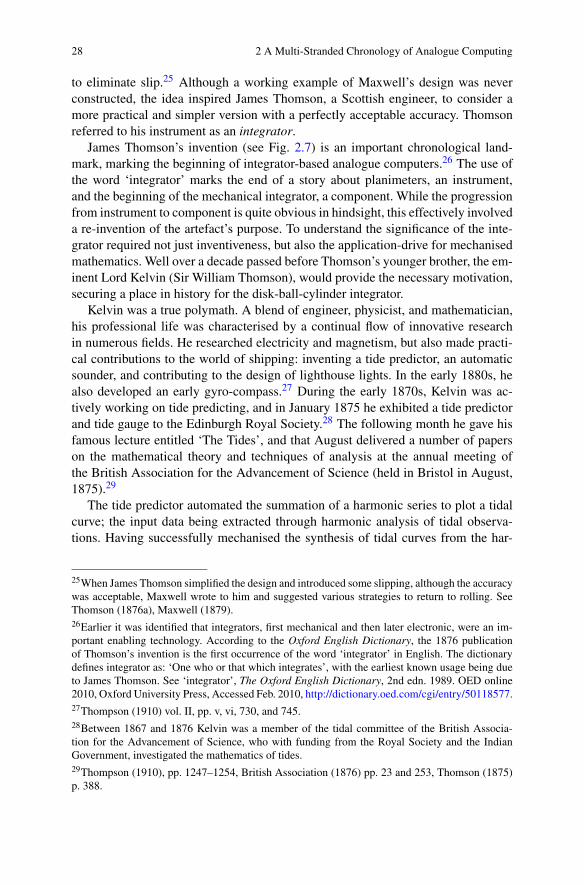
to eliminate slip.25 Although a working example of Maxwell’s design was neverconstructed, the idea inspired James Thomson, a Scottish engineer, to consider amore practical and simpler version with a perfectly acceptable accuracy. Thomsonreferred to his instrument as an integrator.

James Thomson’s invention (see Fig. 2.7) is an important chronological land-mark, marking the beginning of integrator-based analogue computers.26 The use ofthe word ‘integrator’ marks the end of a story about planimeters, an instrument,and the beginning of the mechanical integrator, a component. While the progressionfrom instrument to component is quite obvious in hindsight, this effectively involveda re-invention of the artefact’s purpose. To understand the significance of the inte-grator required not just inventiveness, but also the application-drive for mechanisedmathematics. Well over a decade passed before Thomson’s younger brother, the em-inent Lord Kelvin (Sir William Thomson), would provide the necessary motivation,securing a place in history for the disk-ball-cylinder integrator.

Kelvin was a true polymath. A blend of engineer, physicist, and mathematician,his professional life was characterised by a continual flow of innovative researchin numerous fields. He researched electricity and magnetism, but also made practi-cal contributions to the world of shipping: inventing a tide predictor, an automaticsounder, and contributing to the design of lighthouse lights. In the early 1880s, healso developed an early gyro-compass.27 During the early 1870s, Kelvin was ac-tively working on tide predicting, and in January 1875 he exhibited a tide predictorand tide gauge to the Edinburgh Royal Society.28 The following month he gave hisfamous lecture entitled ‘The Tides’, and that August delivered a number of paperson the mathematical theory and techniques of analysis at the annual meeting ofthe British Association for the Advancement of Science (held in Bristol in August,1875).29

The tide predictor automated the summation of a harmonic series to plot a tidalcurve; the input data being extracted through harmonic analysis of tidal observa-tions. Having successfully mechanised the synthesis of tidal curves from the har-

25When James Thomson simplified the design and introduced some slipping, although the accuracywas acceptable, Maxwell wrote to him and suggested various strategies to return to rolling. SeeThomson (1876a), Maxwell (1879).26Earlier it was identified that integrators, first mechanical and then later electronic, were an im-portant enabling technology. According to the Oxford English Dictionary, the 1876 publicationof Thomson’s invention is the first occurrence of the word ‘integrator’ in English. The dictionarydefines integrator as: ‘One who or that which integrates’, with the earliest known usage being dueto James Thomson. See ‘integrator’, The Oxford English Dictionary, 2nd edn. 1989. OED online2010, Oxford University Press, Accessed Feb. 2010, http://dictionary.oed.com/cgi/entry/50118577.27Thompson (1910) vol. II, pp. v, vi, 730, and 745.28Between 1867 and 1876 Kelvin was a member of the tidal committee of the British Associa-tion for the Advancement of Science, who with funding from the Royal Society and the IndianGovernment, investigated the mathematics of tides.29Thompson (1910), pp. 1247–1254, British Association (1876) pp. 23 and 253, Thomson (1875)p. 388.



Fig. 2.7 The Thomson ‘Integrator’ employed a wheel and sphere mechanism. It is similar to theWetli wheel-and-disk mechanism but uses some of the enhancements of pure rolling that Maxwellargued were so important. Source: Thomson (1876a)

monic base data, Kelvin desired to automatically generate this data. His engineer-ing brain yearned for a machine that could extract the harmonic components ofan arbitrary function. On his return from the Bristol meeting, Kelvin discussed theproblem with his brother, determined to find a solution for what he thought ‘oughtto be accomplished by some simple mechanical means.’30 He outlined his ideas toThomson, who in return mentioned the disk-ball-cylinder integrator. In a flash ofinspiration Kelvin saw how the mechanical integrator could offer ‘a much simplermeans of attaining my special object than anything I had been able to think of pre-viously.’31

From this revelation, Kelvin moved with rapid speed and within days, four in-fluential papers were prepared to be given before the Royal Society of London.32

The first was written by Thomson and described his integrator in detail, the remain-der were by Kelvin and discussed its application. These papers, published in early1876, testified to the significance of the mechanical integrator: broadcasting to theworld of science that it was now possible to integrate products, solve second orderdifferential equations, and with a particular set-up, solve differential equations of an

30Thomson (1876b) p. 266.31Thomson (1876b) p. 266.32These papers were communicated to the Royal Society by Kelvin. A few years later (in 1878)James would, like his brother and father before him, be elected to FRS.


Fig. 2.8 Line drawing of the Kelvin harmonic analyser. Source: Scott and Curtis (1886)

arbitrary order.33 Kelvin’s final paper concluded with a powerful remark about theinvention’s significance:

Thus we have a complete mechanical integration of the problem of finding the free motionsof any number of mutually influencing particles, not restricted by any of the approximatesuppositions which the analytical treatment of the lunar and planetary theories requires.34

It was not long before this insight was engineered into the harmonic analyser,a machine that ‘substitute[d] brass for brain in the great mechanical labour of cal-culating the elementary constituents of whole tidal rise and fall’.35 The harmonicanalyser (see Fig. 2.8) was used to derive the composite harmonics of tidal data, andalso to solve equations for the Meteorological Office.36 As a technology, it usheredin a new genre of calculating instrument: the continuous calculating machine.37

33Thomson (1876a, 1876c, 1876d).34Thomson (1876d) p. 275. Note that this was only a theoretical result. To employ the integratorsin this way would require torque amplification.35Thomson (1882) p. 280.36After its exhibition, Kelvin’s model analyser was transferred to the Meteorological Office whereit was ‘brought immediately into practical work.’ After preliminary trials, a ‘favourable report’was submitted to the Meteorological Council and the council agreed purchase a full-size machineconstructed. The new machine, delivered in December 1879, was first put to use in the ‘determi-nation of temperature constants.’ The results were compared to those measured from photographicthermograms, and others determined through numerical calculations. Previous work had used apolar planimeter to determine a mean value of these plots, the harmonic analyser allowed for moresophisticated processing. The test was successful: ‘. . .the accordance is so very close as to provethat the machine may safely be trusted to effect reductions which could only otherwise be ac-complished by the far more laborious process of measurement and calculation.’ Scott and Curtis(1886), p. 386, Thomson (1878).37Special purpose analogue machines that could extract harmonics continued to be adapted andreworked well into the following century. Examples of mechanical harmonic analysers were de-veloped by Hele-Shaw in the late nineteenth century. For instance Fisher (1957) described howR. Pepinsky, working at Pennsylvania State College had, in 1952, developed ‘a very large com-puter capable of performing directly two-dimensional Fourier syntheses and analyses’ (p. 1.5).Also, it was through the development of a harmonic analyser in the 1930s that Mauchly, one of themajor pioneers of the ENIAC, would begin his career in computing.


2.3.3 1870–1900: The Age of the Continuous Calculating Machine

The latter half of the nineteenth century was a period of intense innovation for thosedeveloping calculating aids, and it was in this period that ‘discrete’ calculating de-vices became common. Two inventions of particular significance to the history ofdiscrete calculators were the variable toothed gear by Frank S. Baldwin (and itsEuropean equivalent invented by Willgodt Odhner), and Dorr E. Felt’s key-drivenmechanism (developed in the 1880s). These technologies paved the way for com-mercial products such as the Brunsviga calculator and the Comptometer.38

In the context of this rapidly developing calculating technology, new machinesinspired the creation of classifications, as well as debate over the ‘proper’ approachto designing such mechanisms. The phrase ‘continuous calculating machine’, a fore-runner of ‘analogue computer’, was coined by those making technical distinctions.39

It was used within the British scientific circle to refer to devices like the planimeterand the harmonic analyser which represented data as a continuous physical quantity.

2.3.3.1 1885: H.S. Hele-Shaw and H.P. Babbage: An Early Analogue–DigitalDebate

A major part of the history of analogue computing are the debates that analogueusers and inventors had with their digital counterparts. Even before the two cate-gories of computer were firmly defined, people posed questions and had discussionsabout what the ‘best’ approaches to mechanising calculation might be. At a meetingof the Physical Society of London in April 1885, we can find a particularly interest-ing example of such a debate between two well-known characters in the history ofcomputing. On the digital side, we find Henry Prevost Babbage, the youngest sonof Charles Babbage.40 Arguing for analogue (then called ‘continuous’) is ProfessorHenry Selby Hele-Shaw, an eminent engineer and inventor of a number of analoguecomputing mechanisms.

Then working at the Royal School of Mines (Now part of Imperial College, Lon-don), Hele-Shaw had advanced the design of integrator mechanisms and understood

38Aspray (1990c) pp. 51–54.39At this time ‘analogue’ would have referred solely to analogy.40Despite his father’s pioneering work on computing, Henry’s interest in computing came laterin life. Henry spent most his career with the East India Company’s Bengal Army. He returned toEngland in 1874 and, in retirement, continued to promote his father’s work on calculating engines,publishing an account of them in 1889. During the 1880s he also assembled some remaining frag-ments of the difference engine and gifted them to several learned institutions including Cambridge,University College London, and Harvard University. Henry’s obituary in The Times refers to pub-lications in subjects including occulting lights and calculating machines, topics that had been ofgreat interest to his father. See Anon. (1918a, 1918b), Babbage (1915) p. 10–11, Hyman (2002)p. 90. The ‘fragment’ of calculating wheels given to Harvard would later provide an interestinglink between Babbage and Howard Aiken’s Harvard Mark I, an early electro-mechanical computerconstructed in the 1940s. Henry died in January 1918, aged 93. See Swade (2004), Cohen (1988).


the distinction between such devices and the numerical calculating machines avail-able for basic arithmetical tasks. At this meeting of the Physical Society, he waspresenting a paper that provided a comprehensive review of all the various classesof mechanical integrator. While his paper is an interesting source for understandingthe various technologies available for mechanising integration, it was in the dis-cussion of that paper (transcribed in the society’s Proceedings) where our ‘debate’occurred. Henry Babbage’s comments, directed towards Hele-Shaw, are perhaps theearliest example of such a debate.41

Major-General H.P. Babbage remarked that which most interested him was the contrast be-tween arithmetical calculating machines and these integrators. In the first there was absoluteaccuracy of result, and the same with all operators; and there were mechanical means forcorrecting, to a certain extent, slackness of the machinery. Friction too had to be avoided. Inthe other instruments nearly all this was reversed, and it would seem that with the multipli-cation of reliable calculating machines, all except the simplest planimeters would becomeobsolete.. . .

[Professor Shaw] was obliged to express his disagreement with the opinion of GeneralBabbage, that all integrators except the simplest planimeters would become obsolete andgive place to arithmetical calculating machines. Continuous and discontinuous calculatingmachines, as they had respectively been called, had entirely different kinds of operation toperform, and there was a wide field for employment of both. All efforts to employ a merecombination of trains of wheelwork for such operations as were required in continuousintegrators had hitherto entirely failed, and the Author did not see how it was possible todeal in this way with the continuously varying quantities which came in to the problem. Nodoubt the mechanical difficulties were great, but that they were not insuperable was provedby the daily use of the disk, globe and cylinder of Professor James Thomson in connectionwith tidal calculations and meteorological work, and, indeed this of itself was sufficientrefutation of General Babbage’s view.42

Was Henry Babbage correct to criticise Hele-Shaw’s view of continuous calcu-lators? In many ways, Babbage should be respected for his commitment to digital,because in the long term his view ran true. However, since a reliable digital com-puter was not to be invented until the 1940s, Hele-Shaw’s position would remaindominant for many years. While the potential benefits of digital could be seen byvisionaries, many advances in technology, coupled with a significant research bud-get, would be needed to realise the digital vision.

The concerns, articulated by Babbage, of the consistent and reliable accuracyavailable with digital computing would be at the centre of arguments for the digitalapproach well into the 1960s. Similarly, Hele-Shaw’s position, that both technolo-gies had their place (each being suited to different purposes), would be a commonresponse of analogue proponents throughout the following century.

41Of course, this is really a continuous-discontinuous debate. The exchange focuses solely oncontinuity and could not be any broader until the first and second thematic time-lines blendedtogether.42Shaw (1885) pp. 163–164.


2.3.4 1880–1920: The Integrator Becomes an EmbeddedComponent Initiating Associations Between Controland Calculation

While Kelvin’s innovation had enrolled planimeter mechanisms into the techno-logical genre of calculating machines, integrators also had to be re-invented as anembedded component. As well as being used in calculating devices, mechanical in-tegrators would become embedded in real-time calculation systems, initiating theclass of technology known today as control systems. However, in the 1800s therewas no general purpose culture and it was not obvious that the technology of acalculating machine could become part of a control mechanism. Essentially, eachnew application of integrators needed to be discovered. One good example of thisis the Blythswood indicator, a simple device based on a cone mechanical integrator,used to determine the speed of a ship’s propeller (or its speed relative to a secondpropeller).

2.3.4.1 1884: Determining the Engine Speed of a Royal Navy Warship:The Blythswood Speed Indicator, an Example of an EmbeddedIntegrator

In a paper communicated to the Physical Society of London, engineers Sir ArchibaldCampbell and W.T. Goolden describe a device developed for measuring the angularvelocity of a propeller shaft. The text records how on a visit to the Dockyards of theRoyal Navy in 1883 they had been drawn to the ‘very urgent need’ for an enginespeed indicator that did not rely on gravity.43 To offer increased speed and manoeu-vrability, ships were being built with two engines driving separate propellers. Thisled to the difficulty that two separate engineering systems had to be coordinated,a challenge when they were located in separate engine rooms. The idea behind theBlythswood indicator was to automatically measure the speed of the propellers, andto communicate the data back to a central location from where both engine roomscould be managed.

The speed indicator employed a cone and wheel in the same way as the planime-ters had done previously (see Fig. 2.9). The cone was rotated at a steady speed andthe wheel shaft at engine speed, forcing the wheel to travel along the surface of thecone until the mechanical constraints imposed by the integrator were satisfied. Thespeed of the engine was read by measuring the displacement of this wheel (integrat-ing a velocity results in a displacement). The inventors then used a series of electri-cal contacts to sense the location of the wheel and drive a repeater instrument at aremote location. With the cone being rotated by clockwork, the instrument could beused to determine the speed of one propeller shaft. Alternatively, if the cone was ro-tated by a second propeller shaft, the instrument would calculate the relative speed.

43Campbell and Goolden (1884) p. 147.


Fig. 2.9 Side elevation of the ‘Blythswood Speed Indicator’, the cone is clearly visible, the wheel(viewed here sideways-on) is halfway along its shaft. Source: Campbell and Goolden (1884).Reprinted with permission of The Institute of Physics

The Blythswood indicator is an early example of embedded analogue computing forcontrol systems.

2.3.4.2 1911: Integrators in Fire Control: Arthur Hungerford Pollenand the Royal Navy

Calculations relating to ballistics problems, such as the trajectories of shells, consti-tute one of the most established uses of applied mathematics. However, during theearly twentieth century advances in gunnery meant that ordinance ranges came to bemeasured in miles rather than yards. Warships now had to engage in battle at greaterdistances; over such distances, variables such as the relative speed and heading ofthe target ship, the ship’s pitch and roll, and wind speed became important factors.Dominance in battle was no longer simply a matter of possessing superior guns orthe fastest ships, naval engagement also demanded advanced computing methods.44

In terms of computation, there were two main approaches to solving the com-plexity: either users were supplied with pre-calculated data, or mechanical comput-ers were installed to provide ‘on the fly’ calculation. The pre-calculated solution wasto tabulate the gun settings for a pre-defined range of important parameters such asair speed, direction or speed of target. The alternative was to build a real-time sys-tem whose mechanism reflected the actual relationships between different variablesin the problem domain and established the correct gun settings. These were knownas fire control systems.45 One of the earliest fire control systems was designed for

44A few decades later, advances in aviation would move the battle ground into the skies, requiringeven faster modelling of three-dimensional dynamics.45Computation on the fly needed to operate at high speed, an application that digital technologycould not begin to address until after World War II. It was much easier and faster if calculations


the British Royal Navy by Arthur Hungerford Pollen. Pollen had invented a numberof weapons systems for warships and had in 1904 been introduced by Kelvin to theThomson integrator. So when Pollen turned his mind towards the problems of firecontrol, it was with integrators that he pieced together his system.46

2.3.4.3 1915: Technology Transfer: Elmer Sperry, Hannibal Ford and FireControl in the US Navy

Despite Pollen’s invention, fire control would initially find a more natural home onAmerican warships. The principal inventor of the analogue computers used for firecontrol in the US was Hannibal Ford who, in 1903, had graduated from Cornellwith a degree in mechanical engineering. His first employer was the J.G. WhiteCompany, where he developed mechanisms to control the speed of trains on theNew York subway. In 1909 Ford began working for Elmer Sperry, assisting withthe development of a naval gyroscope. When Sperry formed the Sperry GyroscopeCompany the following year, Ford became both its first employee and chief engi-neer. Within Sperry, he enjoyed working closely with the US Navy developing earlyfire control technology, and this eventually resulted in the establishment of his ownventure, the Ford Instrument Company, in 1915.47

While working at Sperry, Ford had been given access to the designs of the Pollensystem and so it is perhaps unsurprising that his integrator was also derived fromthe Thomson integrator. Drawing from his expertise on speed controllers, he madesignificant modifications to improve the torque output of the integrator, principallyby adding an extra sphere and compressing the mechanism with heavy springs (seeFig. 2.10).48

2.3.5 1920–1946: The ‘Heyday’ of Analogue Computing?

During the inter-war years, application of mechanical analogue computers flour-ished and became an important part of the warfare technologies employed in World

could be embedded into an artefact. This is not a new concept, for example, a simple instrumentrecently uncovered from the wreck of the Mary Rose used a stepped rule to encode the size of shotand amount of gun powder required for a variety of guns (Johnston 2005). Gunnery resolvers werealso used in anti-aircraft defence, see Bromley (1990) pp. 198–159.46See Pollen and Isherwood (1911a, 1911b), and Mindell (2002) pp. 38–39. Pollen found it difficultto sell his idea to the Royal Navy, which had very conservative views towards automation. Thisconservatism would not be sustainable. May 1916 saw the World War I sea battle of Jutland, a nowfamous defeat for the Royal Navy, who were unable to compete against the German long rangegunnery. Their defeat was partly due to a lack of gunnery computing devices, and Mindell noteshow the one ship that was fitted with the Pollen system out-performed the rest of the fleet. SeeMindell (2002) pp. 19–21.47Mindell (2002) pp. 24–25.48Ford (1919/1916a), Clymer (1993) pp. 24–25, and Mindell (2002) pp. 37–39.


Fig. 2.10 Images fromHannibal Ford’s patent for anintegrator. The disk andcylinder inherited from theThomson integrator areclearly visible. Source: Ford(1919/1916a). Ford’sintegrator employed a springto compresses the disk on to adouble-sphere mechanism,delivering maximum torque,an invention for which Fordwas granted a second patent(Ford 1919/1916b)

War II. As a consequence, historians have christened this pre-1946 period a ‘heyday’of analogue computing.49 During this period there was simply no digital competi-tion, thus analogue computing was computing. This would remain the case until theemergence of electronic digital computers in World War II research programmes. Interms of the technology’s use, David Mindell described World War II as ‘analog’sfinest hour’.50

49As exemplified by Campbell-Kelly and Aspray (1996), this was based on the observation thatmany archetypal analogue computers (e.g. the differential analyser) dominated in this period. Small(2001) countered this idea because it contributed to the historical devaluation of post-war analoguecomputers. However, labelling this period a ‘heyday’ does not have to imply that there was nosuccessful post-war story.50Mindell (2002) p. 231.


2.3.5.1 1931: Vannevar Bush and the Differential Analyser

Although Kelvin had conceived of how mechanical integrators could be connectedtogether to solve differential equations, a full realisation of the idea would notemerge until the differential analyser was developed in the 1930s. The solution ofhigher order differential equations required the output of one integrator to drive theinput of another (integrating the result of a previous integration). Even more prob-lematic was that automatically solving an equation required a feedback loop andKelvin lacked the required torque amplifier. The torque amplifier used in the differ-ential analyser was developed by Niemann at the Bethlehem Steel Corporation.51

Vannevar Bush (1870–1974) is well known for his contribution to twentieth cen-tury American science. Alongside his technical ingenuity, he was a superb admin-istrator and during World War II was the chief scientific adviser to President Roo-sevelt.52 Bush’s involvement with analogue computing began during his Masters de-gree when he developed the profile tracer, an instrument which, when pushed along,used a mechanical integrator to record changes in ground level. He joined MIT in1919, and initiated a research program that developed a variety of integrator-basedcalculating machines including the Product Integraph developed between 1925 and1927, and the differential analyser.53

The differential analyser was completed between 1930 and 1931. It consisted ofa large table with long shafts running down the centre. Alongside were eight me-chanical integrators and a number of input and output tables. By using the differentshafts to connect together the inputs and outputs of the different functional com-ponents, it was possible to construct a system whose behaviour was governed by adifferential equation (see Fig. 2.11).54 The differential analyser was an exceedinglypopular instrument and many copies were made and installed in research centresacross the world. During the late 1930s, MIT received funding from the Rockefellerfoundation to construct a larger and more accurate machine. The Rockefeller anal-yser still employed mechanical integrators, but used servo mechanisms to speed upthe programming of the machine.55

51The torque amplifier works in a similar way to a ship’s capstan, allowing a small load to con-trol a heavier load. Various means of torque amplification were used in the differential analysersand in later years the Niemann amplifier was replaced by electrical and optical servomechanisms.Bromley (1983) p. 180, Fifer (1961) vol. III, pp. 665–669, and Mindell (2002) pp. 158–159.52There are many correspondences between Bush and Kelvin. Both were successful scientists andtechnologists. Each not only advanced their field, but also became known for their successful man-agement of large projects. Kelvin was directly involved in the successful laying of an Atlantictelegraph cable in 1865. See Smith (2004).53Campbell-Kelly and Aspray (1996) pp. 53–54, Small (2001) p. 41, Mindell (2002) pp. 153–161,Wildes and Lindgren (1985) pp. 82–95.54An accessible introduction to the differential analyser (with diagrams) is given by Bromley(1990). A number of differential analysers were constructed out of Meccano (See Chap. 5, p. 99)and had reasonable accuracy.55See Owens (1996), Mindell (2002) pp. 170–173.


Fig. 2.11 A ‘program’ for the differential analyser of a free-fall problem. Each linkage betweenshafts corresponded to a different mathematical operator in the original equations. Based on anexample given in Bush (1931) p. 457

As an icon of mathematical mechanisation, the differential analyser became afocal point in the formation of early computing culture. In an introductory article tothe first issue of the Journal of the ACM, Samuel Williams, the fourth president ofthe Association of Computing Machinery (ACM), referred to the 1945 MIT confer-ence where the Bush-Caldwell differential analyser was first publicised as the ‘firstmeeting of those interested in the field’. For Williams, the differential analyser wascentral in the formation of the ‘automatic computing’ community.56

In an address to the American Mathematical Society, Vannevar Bush presentedthe differential analyser as an instrument that provided a ‘suggestive auxiliary toprecise reasoning’.57 His belief was that the machine could provide significant cog-nitive support for mathematical work and he fully expected this ‘instrumental analy-sis’ to become a major approach in mathematics. In his autobiography he describedthe differential analyser’s educational dimension, which allowed the calculus to becommunicated in mechanical terms. Here, both the referent and analogy were sowell accepted that the set-up began to communicate knowledge about the relation-ship between them. For Bush’s draftsman, the differential analyser provided a phys-ical insight into dynamic problems without need for mathematical formulation.

56See Williams (1954) p. 1, Care (2007b).57Bush (1936) p. 649.

2.4 From Analogy to Computation: the Development of Electrical Modelling 39

As an example of how easy it is to teach fundamental calculus, when I built the first dif-ferential analyzer. . . I had a mechanic who had in fact been hired as a draftsman and as aninexperienced one at that. . . I never consciously taught this man any part of the subject ofdifferential equations; but in building that machine, managing it, he learned what differen-tial equations were himself. He got to the point that when some professor was using themachine and got stuck—things went off-scale or something of the sort—he could discussthe problem with the user and very often find out what was wrong. It was very interesting todiscuss this subject with him because he had learned the calculus in mechanical terms—astrange approach and yet he understood it. That is, he did not understand it in any formalsense, but he understood the fundamentals; he had it under his skin.58

On reflection, ‘differential analyser’ was an interesting name to choose for thismachine, and a number of other prominent members of the computing commu-nity questioned this choice of terminology. For instance, In January 1938, Dou-glas Rayner Hartree gave a talk to the Mathematical Association. He argued thatthe name of the differential analyser was, as he wrote, ‘scarcely appropriate as themachine neither differentiates nor analyses, but, much more nearly, carries out theinverse of each of these operations.’59 Similarly Hollingdale and Toothill (1970)suggested that a better name might have been ‘integrating synthesizer’. In describ-ing how the machine was used they noted that mathematical expressions were builtup ‘term by term’ and that this process was ‘hardly a process of analysis’.60 Thus wecan see that when thinking about the nature of computing, the distinction betweenanalysis and synthesis was an important contrast to make. George Philbrick, anotherpioneer of analogue computing, also observed that not all computing was analysis,advocating synthesis as part of his ‘lightning empiricism’.61

The differential analyser is a good place to complete this time line. We have seenhow the demands for calculation inspired the creation of a number of analogue de-vices such as planimeters and integrators. These devices were then aggregated intolarger systems for equation solving, such as the differential analyser. However, notall analogue devices were used to solve equations. The following time line describesthose used for modelling: machines where synthesis, not analysis, was the centralconcern.

2.4 Second Thematic Time-Line—From Analogyto Computation: the Development of Electrical Modelling

As previously described, there are two main aspects to analogue computing: con-tinuous representation and physical analogy. In the last section, the history of themechanical integrator gave us a story of the continuous calculating machine. In this

58Bush (1970), p. 262.59Hartree did however concede that since it was Bush’s ‘child’, he had ‘the right to christen it’. SeeFischer (2003) p. 87.60Hollingdale and Toothill (1970) pp. 79–80.61See Sect. 4.3.1, p. 86, below.


section, we turn to the tradition of analogue computing that emphasises the con-struction of analogies.

In a sense, analogue computers based on analogy are more closely related to nat-ural science experimentation than to the history of calculating machines. Scientistshave for generations constructed models to illustrate theories and to reduce complexsituations into an experimental medium. Since the mid-nineteenth century, the tech-nology available for creating models (or analogies) gradually became part of thehistory of computing: developing from ad-hoc laboratory set-ups into sophisticated,general purpose tools.

2.4.1 1845–1920: The Development of Analogy Methods

During the nineteenth century, model construction embraced the new medium ofelectricity. Electrical components offered improved flexibility and extended thescope of what could be represented in a machine. In many ways, the history ofthe development of modern computing is also the history of ongoing attempts tomanage an electrical (and later electronic) modelling medium.

In the context of direct analogue computing, this modelling medium took twoforms: analogues were either based on circuit models, of which the network anal-yser became an archetype; or alternatively, an analogue was established by exploit-ing the physical shapes and properties of a conducting medium such as conduct-ing paper or electrolytic tanks.62 Electrolytic tanks offered a continuous conductivemedium while resistance networks had a necessarily discrete representation of theflow space.63 Together, these techniques became grouped under the umbrella con-cept of ‘electrical analogy’. Analogue models were first referred to as ‘electricalanalogies’, and then later as ‘electrical analogues’. Gradually, the experimentalistculture of the laboratory was replaced by more generic technologies, laying thefoundations for approaches based on physical analogy to become computing tech-nology.

2.4.1.1 Tracing Field Lines, Field Analogies and Electrolytic Tanks

A whole class of analogue computing was dedicated to the modelling of field po-tentials. These analogues were typically used for solving problems that would oth-erwise have required the solution of partial differential equations. They employed

62As well as tanks and networks, other novel media were employed, for instance the Hydrocal,a research analogue developed at the University of Florida around 1950, was based on pipes andtanks of fluid (Anon. 1951b, p. 864). Typically, the applications that employed an indirect computermoved to digital more quickly because the problems were already in a mathematical form thatcould be programmed. For direct analogue computers, the transition took longer because a suitableand trustworthy digital representation had to be established.63Note that this starts to frustrate certain clear-cut definitions of analogue computing. Contempo-rary actors were using the labels ‘discrete analogue’ and ‘continuous analogue.’


the principle that heat flow, aerodynamic flow, and a whole class of other problemsgoverned by Laplace’s equation, could be investigated through the analogous dis-tributions of electrical potential in a conductive medium such as conductive paperor an electrolytic tank. The identification that lines of electrical flux could representflow dates back to early work by the German physicist, Gustav Robert Kirchhoff.In 1845 Kirchhoff used conducting paper to explore the distribution of potential inan electrical field. The so-called ‘field plot’ turned an invisible phenomenon into avisual diagram and allowed scientists to begin exploring the analogy between fluidflow and electrical fields.64

Electrolytic tanks were the logical extension of paper-based field plots. In 1876,in the same volume of the Proceedings of the Royal Society that Kelvin publishedhis account of the use of integrators to solve differential equations, a differentform of modelling technology was communicated to members of the Royal Soci-ety. This was an electrolytic tank developed by the British scientist William GryllsAdams, the younger brother of the astronomer who co-discovered the planet Nep-tune. Adams spent most of his academic career at King’s College, London, wherehe established its Physical Laboratory (1868) and actively pursued the teaching andresearch of experimental physics.65 Initially part of the material culture of experi-mental physics, electrolytic tanks would later become an important technology ofanalogue computing.

Adams’ electrolytic tank further contributed to the visualisation of electrical fieldlines. The apparatus consisted of a wooden tank containing water, two fixed metalelectrodes, and two mobile electrodes. Connecting an alternating electrical currentto the fixed electrodes established an electrical field which could be explored withthe mobile electrodes (see Fig. 2.12). A galvanometer connected in series showedthe difference in electrical potential between the two mobile electrodes, and thisallowed these roaming probes to be used to find points of equal electrical potential(signified by a zero displacement of the galvanometer needle).66 In this way gradientlines of an electrical field could be mapped.

64Small (2001) p. 34. As well as conductive electrolyte, conductive ‘Teledeltos’ paper was alsoused extensively during the 1950s and 1960s.65Adams joined King’s College firstly as a lecturer, and subsequently held the chair of natural phi-losophy between 1865 and 1905. This position had been previously held by James Clerk Maxwell.Adams was an active member of the London scientific scene. He was elected Fellow of the RoyalSociety in 1872 and was a founding member of the Physical Society of London (now the Instituteof Physics) for which he acted as president between 1878 and 1880. During 1898 Adams servedon the council of the Royal Society and in 1884 was president of the Society of Telegraph Engi-neers and Electricians (later the Institution of Electrical Engineers). In 1888, Cambridge Universityawarded him a DSc. See Anon. (1897b, 1915), G.C.F. (1915), Anon. (1897a, 1888). His empha-sis on experimental methods is an interesting link with other actors in this history, such as theengineers Vannevar Bush and George Philbrick, as well as the meteorologist, Dave Fultz.66See Adams (1876).


Fig. 2.12 A diagram of Adams’ electrolytic tank from his original paper. The fixed electrodes aremarked A and B , the mobile electrodes are connected to the T-shaped handles. Source: Adams(1876). Reproduced courtesy of the Royal Society

2.4.1.2 Miniature Power Networks and Resistor-Capacitor Models

Another important technology was electrical network models, also originating in thenineteenth century. For instance, in the 1880s Thomas Edison, the inventor of thelight bulb, employed a research assistant to build scale models of power networks.Initially one-off models, over a number of years electrical networks evolved frombeing special purpose laboratory experiments into more general purpose set-ups.Subsequently, these electrical analogues were replaced by programmable analoguecomputers, before a final transition to programmable digital computers was madeduring the 1960s and 1970s.

2.4.2 1920–1946: Pre-digital Analogue Modelling

It was during the 1920s that electrical analogy became properly established as amodelling medium and a number of contemporary publications regard an early pa-per by the engineer Clifford A. Nickle as a seminal development. In this paper,Nickle articulated a general approach to developing electrical models of complexsystems, initiating the uptake of electrical analogue methods in engineering.67 Itwas around this time that analogue culture was beginning to stabilise, allowing thediscipline of electrical analogy to become enclosed and established. As a result,electrical network analogues became part of the literature of computing.68 The his-

67See, for instance, Nickle (1925) or Karplus and Soroka (1959).68This is shown in the annual subject indexes of the Review of Scientific Instruments, a journalpublished by the American Institute of Physics during this period. Between 1947 and 1950, the


tory of the enclosure and stabilisation of the analogue discipline will be covered inChap. 4.

The following sections outline some major landmarks in analogue modelling be-tween 1920 and 1950, including: the development of electrical networks, electrolytictanks in France, the modelling culture associated with high-speed analogue circuits,and the electrical modelling of oil reservoirs.

2.4.2.1 1924: The Origins of the MIT Network Analyser

Resistance network analogue computers had their origins in the pre-war work onelectrical networks at MIT. In particular, the network analyser was designed to rea-son about full scale electrical supply networks in miniature by analogy.

Just as Edison had constructed scale models during the 1880s, researchers atMIT began to build special purpose models to assist with the design of new powerdistribution networks.69 Developing an individual model for each network was notvery flexible and researchers realised that they needed a more generic tool. Thenetwork analyser occupied a large room and through its patch panels it allowed auser to quickly set up a specific network. Initially the analyser was used just toreason about electrical supply networks in miniature. However, its users soon de-veloped techniques for wider modelling applications, representing more exotic ref-erents (such as hydraulic systems) within the framework of resistor-capacitor net-works. It is clear that contemporary users saw this technology more as a modellingtool than equation solver. For example, Bush described the network analyser as aninstrument in which whole equations mapped to a particular set-up. By contrast, heunderstood that the differential analyser established analogies between the machineand individual components of a differential equation.70

Resistor-capacitor circuits could also be harnessed to directly solve mathemati-cal equations. For instance, during the early 1930s, the Cambridge scientist RawlinMallock devised an electrical device to solve simultaneous equations. Using trans-former winding ratios to mirror relationships in a set of mathematical equations,Mallock was able to directly extract a solution through measurement. Mallock de-veloped an experimental machine in 1931 and the construction of a full-size ma-chine (capable of solving ten simultaneous equations) was completed in 1933.71

number of articles classified under ‘computer devices and techniques’ grew to encompass bothelectrical networks and more conventional analogue computers. The growth of this section is notsimply due to advances in the technology. Instead we can see that there is an enclosure of theidentity of ‘computing technology’—the older classifications of ‘electrical network’ and ‘countercircuits’ that existed in 1947, being either reduced in size, or removed by the early 1950s.69This was in part due to the expansion and amalgamation of American regional power grids duringthe 1920s. The complexities of large scale transmission networks caused unstable black-holing inthe power grid. See Akera (2007) p. 31.70See Bush (1936).71A patent application was submitted in 1931, and granted in March 1933 (Mallock 1933/1931).Later that month Mallock submitted a paper describing the machine in the Proceedings of the RoyalSociety (Mallock 1933).


Because it modelled mathematical equations, the Mallock machine is a fine ex-ample of the kind of analogue device known as ‘indirect’. Each equation was mod-elled by a circuit connecting a number of transformers; the number of transformerscorresponding to the number of variables in the equation.72 Vannevar Bush wasimpressed with the technique of using transformers, and used it as a starting pointfor further work in circuit models.73 Although Mallock’s machine was intended asan indirect equation-solver, Bush would make significant use of its principles inthe development of methods for structural analysis, an example of direct analoguecomputing. This blurring of the two types of analogue computation was typical ofBush’s approach to computing. At MIT the two perspectives of analysis and synthe-sis were managed within one research program.74 We will return to this ‘blurring’ inthe third thematic time-line, but first we need to consider other important analogy-making technologies.

Techniques using resistance networks were particularly useful in geographicalmodelling (such as hydrological planning) because the layout of the problem couldphysically map to the geography of the real-world problem. The co-evolution ofnetwork analysers and machines based on integrators came together in the researchat MIT, where both network and differential analysers were developed. These de-velopments marked the beginning of the entwinement between analogy and calcula-tion; a mixture of mathematics and experiment that would become blended in ‘ana-logue computing’. The two types of analyser represented different activities—twoperspectives of use—sub-dividing the analogue computing class. Small describedthem as competitive technologies that ‘maintained distinct lineages, but neverthelessshared a similar conclusion; their displacement by electronic digital computers.’75

2.4.2.2 1932: Le Laboratoire des Analogies Electriques: Electrolytic Tanksin France

So far we have mainly reviewed the Anglo-American story, however, there was sig-nificant parallel activity in other countries. One particularly interesting exampleis the work of the French mathematician Joseph Pérès (1890–1962) who became

72The coefficients of each variable were ‘programmed’ by the number of windings connecting thattransformer to the others—clockwise windings for positive coefficients, and anti-clockwise fornegative. Through applying an alternating current supply to one of the coils, the electrical circuitswould reach a steady state corresponding to the equations’ solution.73See Bush (1934).74Mindell (2002) describes how Bush’s two perspectives of ‘modeling’ and ‘calculation’ wereheld in tension, indicating that this was the beginning of an entwinement between the empiricalapproaches of analogy making, simulation, and modelling; and the analytical approaches of calcu-lation, theory and mathematics. Bush had a natural leaning towards the use of analogies. This canbe seen in his earlier work on gimbal stabilisation (Bush 1919). See Mindell (2002) pp. 149–150,Akera (2007) pp. 31–32, Owens (1986), Wildes and Lindgren (1985) pp. 86–87.75Small (2001) p. 40.


well-known for his use of electrolytic tanks to model physical systems.76 In 1921Pérès had been appointed Professor of Rational and Applied Mechanics at Mar-seilles where he was inspired by the analogue modelling of his colleague J. Valensi.Valensi had been working on a fluid dynamic problem by employing an analogybetween streamlines of fluid flow and potentials in an electrical field.77

By 1930, Valensi and Pérès had founded the Institute of Fluid Mechanics atMarseilles and over the following years, applied electrolytic tanks as a computingtechnology. Around 1932 Pérès accepted a Chair at the Université Paris-Sorbonnewhere, along with his researcher Lucian Malavard, he established a Department ofElectrical Analogy (Le Laboratoire des Analogies Electriques) within the Paris Fac-ulté des Sciences. In Paris, Pérès and Malavard began to develop various refinementsto electrolytic tank methods. In particular they developed applications using tanksof various depths, a technique that had been employed within British aeronauticalresearch. The outcome of the work was the Wing Calculator, a tank that could solvethe equations governing a lifting wing. The calculator was used by a number of air-craft manufacturers until 1940 when the outbreak of war in Europe prompted thelaboratory to be dispersed and the remaining equipment destroyed.78

The uptake of electrolytic analogue methods in Britain might have been greaterhad the work of Pérès and Malavard not been interrupted during the war years.The post-war re-opening of communication saw British use of the electrolytic tankrapidly increase. The use of tanks in aeronautical research is discussed further inChap. 7.

2.4.2.3 1935: George Philbrick and the Polyphemus: Developmentof Electronic Modelling at Foxboro

Another type of analogue technology arose from the electronic modelling of con-trol systems. This lead to the popular class of machine referred to as the ‘GeneralPurpose Analogue Computer’ (or GPAC). The GPAC was essentially an electronicversion of the differential analyser.

Many of the pioneers of these high speed analogue computers had previouslyundertaken research in control systems analysis or similar fields. One such char-acter was George Philbrick (1913–1974), a Harvard-educated engineer.79 Working

76Pérès came from an academic family and for his doctorate had studied under the supervision ofthe Italian mathematician Vito Volterra. Pérès’ thesis Sur les fonctions permutable du Volterra wassubmitted in 1915.77In 1924, the same year that Valensi used an electrical analogue to represent flow and the MITnetwork analyser was unveiled, similar work was done by E.F. Relf. A future fellow of the RoyalSociety (elected in 1936), Relf held the position of superintendent of NPL’s Aeronautics Divisionbetween 1925 and 1946. He also established the College of Aeronautics at Cranfield. See Pankhurst(1970), Taylor and Sharman (1928).78Pérès (1938), Mounier-Kuhn (1989) p. 257.79Mindell (2002) p. 307, Holst (1982). His obituary describes how he completed the Harvard un-dergraduate program in ‘record time’, entering the school in 1932 and receiving his degree in 1935.


at the Foxboro Corporation, Philbrick developed the Automatic Control Analyzer(ACA) simulator (nicknamed ‘Polyphemus’), an early electronic computer.80 Likemany prominent control engineers, Philbrick worked for the US government as afire control researcher during World War II. Working within Division 7 of the Na-tional Defense Research Council (NDRC), he met several, later eminent, engineerswho were involved in the early seminal work on control electronics and servomech-anisms.81 Once his wartime research was completed, Philbrick had intended to enrolat MIT as a graduate student and develop a high-speed analogue computer. How-ever, this project was indefinitely put on hold when he was approached to design aspecial purpose simulator for the Wright Aeronautical Corporation. He successfullyconstructed the simulator in his spare bedroom and, as a result, set up his own com-pany: George A. Philbrick Researches, Inc. (often abbreviated to GAP/R). GAP/Rwere the first company to manufacture and market a commercial operational am-plifier and later became a major manufacturer of analogue computers.82 Philbrick’sapproach to analogue computing is discussed in Chap. 4.

2.4.2.4 1942: William A. Bruce and the Modelling of Oil Reservoirs

An interesting example of analogue computing as a modelling medium is the appli-cation of electrolytic tanks and resistive networks to the modelling of oil reservoirs.This application dates back to the 1930s, when researchers for large petroleum cor-porations began to develop electrical models of the hydrodynamics of subterraneanoil reservoirs. Within reservoir engineering literature, the first well-known applica-tion of analogue computing to such problems is attributed to William A. Bruce, a re-searcher of Carter Oil. He invented his ‘analyzer for subterranean fluid reservoirs’in 1942, demonstrating that the dynamics of an underground oil reservoir could berepresented by electrical circuits.83

He worked for Foxboro between 1936 and 1942, under the eminent control engineer Clesson E.Mason. Mason was awarded the Rufus Oldenburger Medal for his work on automatic control in1973. See Paynter (1975) and Anon. (2005b).80Similar activities were going on in other engineering contexts. In 1939 Helmut Hoelzer wasworking on early analogue computing as part of German missile research, and in Britain a team de-veloping radar crew trainers at the Telecommunications Research Establishment (TRE) constructedan analogue simulator using electro-mechanical integrators, which they called ‘the velodyne’. TheTRE was central in laying the foundations of post-war analogue computing research. Another sig-nificant research program was American research into operational amplifiers for computing at Belllabs, from which came seminal papers from Ragazzini, Randall, and Russell, whom John McLeodreferred to as the ‘three-Rs’ of simulation. These three had also been involved with the wartimeNDRC analogue culture. See Small (2001) pp. 66–67, 69–71, McLeod (1968) p. 15.81See Mindell (2002) pp. 199–200. Mindell lists a number of important names who worked withinthis research team throughout the wartime period, including the famed J.R. Ragazzini and G. Stib-itz.82Alongside these activities, Philbrick continued to act as a consultant to Foxboro. See Holst (1982)p. 156.83Peaceman (1990) pp. 106–108, Bruce (1947/1943).

2.5 Analogue Computing and the Entwining of Calculation and Modelling 47

Throughout the following two decades, large numbers of patents for reservoiranalysers were granted. Initially, the inventors made no reference to analogue, anal-ogy or computing. Throughout his 1945 patent application, Bruce described his cir-cuits as an ‘electrical counterpart of a reservoir’. However, later reservoir analyserswould be described as ‘electrical analogies’ and thus become part of the history ofanalogue computing. Their story is told in Chap. 6.

2.5 Third Thematic Time-Line—Analogue Computingand the Entwining of Calculation and Modelling

The previous sections described the major technologies considered important to thehistory of analogue computing. However, it was only after the emergence of the dig-ital computer that it became necessary to assemble these various technologies underthe umbrella term of ‘analogue computing’. In the formation of an analogue iden-tity, the two concepts of continuity and analogy were blended together, entwiningthe chronologies of calculation and modelling into a coherent body of technologyand practice.

2.5.1 1940: The Emergence of Analogue Computingas a Technical Label and Class of Machine

According to the Oxford English Dictionary the earliest use of the word ‘analogue’to describe a class of computers occurs in a 1946 article authored by DouglasHartree.84 Published in Nature, the article stated that the classification was estab-lished on the other side of the Atlantic.85 It is assumed that Hartree was introducedto the analogue–digital classification during his visits to the Moore School of Elec-trical Engineering at the University of Pennsylvania. This was possibly from ENIAC

pioneer John W. Mauchly who is known to have used the classification in commu-nication with John Vincent Atanasoff (another pioneer) in 1941.

Mauchly and Atanasoff’s usage is the earliest explicit reference to analogue asa class of computer technology. Indeed, in an autobiographical article, Atanasoffclaimed to have first used the classification a year earlier. He recollected that thedistinction between the two classes of computer ‘came from [his] own mind’ and

84‘Analogue, n., and a.’, The Oxford English Dictionary, 2nd edn. 1989. OED on-line 2010, Oxford University Press, Accessed Feb. 2010, http://dictionary.oed.com/cgi/entry/50007887.85Hartree wrote that ‘the American usage is analogue and digital machines’, (Hartree 1946, p. 500).In fact, Hartree actually preferred to use ‘calculating machine’ for digital and ‘calculating instru-ment’ for analogue, a distinction which he derived from the Encyclopaedia Britannica where the‘two classes of equipment [were] considered in different articles’ (Hartree 1949, p. 1). These werethe articles on ‘calculating machines’ and ‘mathematical instruments’ respectively.




identified a paper describing a digital computing technique (Atanasoff 1940) as theearliest record of his usage.86 In this paper he wrote that ‘he was aware of the pos-sibility of using a mechanical or electrical analogue but discarded this method, asbeing too inaccurate and cumbersome.’87

Atanasoff’s use of the word ‘analogue’ refers to a method of computation, ratherthan a particular class of device, subtly weakening the claim that his publication hadbeen the first reference to analogue as a class of computer. However, the terminol-ogy appears to have crystallised during early 1941, and within a couple of monthsAtanasoff was communicating to Mauchly a definition of analogue computing farmore recognisable as what would later become mainstream. The dialogue betweenAtanasoff and Mauchly began when they first met in December 1940 and resultedin Mauchly visiting Atanasoff in the summer of 1941.88 On his return, Mauchlyprepared some notes in which he described two classes of computing. In these notesattention is drawn to the principle of analogy, and the limited accuracy of analoguetechnology:

Computing machines may be conveniently classified as either ‘analog’ or ‘impulse’ types.The analog devices utilize some sort of analogue or analogy, such as Ohm’s Law or thepolar planimeter mechanism, to effect a solution of a given equation. The accuracy of suchdevices is obviously subject to limitations; at times the attainable is more than sufficient,but there is increasing need for more computational aid not so restricted. Impulse devicescomprise all those which ‘count’ or operate upon discrete units corresponding to the integersof some number system. There is no theoretical limit to the accuracy to which such deviceswill work; practical limitations on the bulk or cost or convenience of operation provide theonly restrictions. The usual mechanical computing machine, utilizing gears, pauls, etc., areexamples of impulse calculators.89

For Mauchly and Atanasoff, the technology they named ‘analog’ was based onphysical analogy. Hence, an analogue was a machine or set-up which maintained acorrespondence or analogy between two physical systems. The continuous natureof the machine was coincidental. A similar emphasis was made by Douglas Hartreewho considered measurement to be a central aspect of his analogue instruments,the technology that operated by ‘. . .translating numbers into physical quantities of

86Atanasoff (1984) p. 234. Although he acknowledges that ‘others may previously have had thesame idea’ about the separation of computers into two classes, Atanasoff (1984) claimed that hehad been ‘the first to use the word analog for computers . . .the term I devised at the time I madethis distinction and used in my 1940 manuscript (spelled there analogue)’. Even the originalityof ‘analogue’ is questionable. David Mindell noted that while Atanasoff ‘may have been the firstto specifically apply the term analog to a computing machine’, others were using analogy to re-fer to earlier circuit models (Mindell 2002, p. 387). Although used for calculation, such circuitswould have not been called computers, so perhaps the real contribution of this 1940 paper was theconnection between the linguistic labels ‘analogue’ and ‘computer’.87Atanasoff (1940) p. 316.88Mauchly (1984) pp. 125–126.89Mauchly (1941)—this usage was attributed to Atanasoff. While Mauchly made no direct refer-ence in these notes to the relationship between analogue computing and the continuous represen-tation of variables, he was aware of the connection. Note his spelling of ‘analog’ for the category,and ‘analogue’ for the concept.


which the numbers are the measures. . . finally measuring some physical quantityto give the result.’90 Even forty years on, Atanasoff retained an emphasis on mea-surement rather than continuity: ‘In analog computers. . .’, he writes, ‘a number isrepresented by a physical quantity in the machine as measured by some system ofunits’.91

2.5.2 1945–1960: The Development and Stabilisation of ComputerTechnology

World War II was a scientific war, and large research funds were distributed to de-velop computing aids for the science and engineering underpinning the war effort.Due to rapid innovation, and secrecy of projects, various different technologicalpaths were pursued, some analogue, some digital.

One of the major technical benefits of the wartime research was the improvementin electronics. During the years after 1945, analog computers were constructed us-ing electronic components, the mechanical integrators being replaced with capacitorcharging circuits. The replacement of the mechanical with electronic was not im-mediate. The electronic components often had a lower accuracy than the precisionengineering of mechanical integrators, but were considerably cheaper and could beused at higher speeds.92 High speed components facilitated a new type of analoguecomputing which supported repetitive operation (or rep-op), where the computercalculated many solutions per second, supporting parameter variation and explo-rative modelling. Rep-op allowed problems to be time-scaled, supporting problemsto be solved via parameter variation. As a piece of contemporary sales literature putit:

Time itself becomes the servant, not the master, enabling protracted processes to be repeatedmany times in a minute or disturbances too fast for the human mind to be examined atleisure.’93

2.5.2.1 The Development of Electronic Differential Analysers

Now unified under ‘analogue computing’, analogues came to be classified as eitherdirect or indirect. The indirect analogues were essentially the developments of the

90Hartree (1947) pp. 7–8. Hartree did refer to continuous data, but not as a defining feature ofanalogue computing. He wrote that ‘analogue machines can be designed to handle continuousvariables, and in particular can handle integration as a continuous process’ (p. 8).91Atanasoff (1984) p. 234. This can provide insight into his use of the phrase ‘direct calculation’which is central to Atanasoff’s understanding of the distinction. Digital computers allow the com-putation to work with numbers directly whereas analogue computing manipulates measures thatrepresent numbers. Atanasoff’s use of direct should not be confused with the two categories ofanalogue computers—direct and indirect—that came later.92Small (2001) pp. 54–56.93EMI (1955–1965).


equation solving tradition. The development of electronic versions of the differen-tial analyser emerged from the wartime work on control systems, which had de-veloped the electronic amplifiers needed to construct an electronic integrator. Onesuch example of a high speed electronic analogue computer was developed by Mac-nee (1949). Similarly research machines were developed in various universities andresearch establishments. In America most post-war analogue computing was organ-ised by the Office of Naval Research (ONR), which organised a number of largeprojects and symposia. In the UK, most of the early research was undertaken inrelation to aeronautics, the large TRIDAC machine becoming operational in 1954.94

On the other hand, the development of direct electronic computing followed thesame path as it had before the war. Much of the work on resistive networks andelectrolytic tanks was focused on specific application domains such as engineer-ing structures and power system analysis. These techniques were used extensivelyfor quick, explorative investigations. Examples include the flutter simulators andelectrolytic tanks used in aeronautics (see Chap. 7), resistance analogues used inhydrology and ground water research (see Chaps. 5 and 6), and modelling electrictransmission networks.

2.5.2.2 Early Digital Computers as the Evolution of Analogue Architectures

Although digital computers are a distinct technology from analogue, it is possibleto see many of the early digital machines as the evolution of an analogue architec-ture. Indeed, if the distinction between analogue and digital only emerged after thedevelopment of digital computing, it makes sense that the earliest machines mightexpose a closer relationship between the two.

Earlier we referred to ENIAC, arguably the first programmable electronic dig-ital computer.95 Although fundamentally a digital machine, ENIAC was in manyways an extension of the analog culture that had existed previously. The choice ofacronym (standing for Electronic Numerical Integrator and Computer) emphasisesthe link. A major application of analogue computers was mechanising the calcu-lus and the ENIAC was intended to solve those problems. Essentially, this machinewas the digital replacement of the differential analyser. An insightful quote fromthe ENIAC patent (submitted in 1947) shows that making an analogue computationwas understood as akin to conducting a laboratory experiment. The digital ENIAC

offered a ‘cleaner’, more mathematical alternative:

It may be noted that much of the present experimental work consists essentially of thesolution of mathematical problems by analogy methods. If one had a computing machine ofsufficient flexibility the necessity for these experiments would be obviated. Our inventionmakes available such a machine.

In discussing the speed of computing machines it is desirable to distinguish betweenso-called continuous variable and digital machines. Although existing continuous variable

94Small (2001) pp. 181–182.95ENIAC ran its first successful program in 1946. It should be noted that deciding which machineswere ‘first’ relies largely on personal definition and is often a contested issue amongst historians.


machines such as the differential analyser and the AC network analyser are exceedinglyrapid, the class of problems which they can solve is limited.96

As can be seen from the quote, the 1940s was the period when the concept of theanalogue computer was introduced to encompass both of the traditions explored inour first two time-lines. Here Eckert and Mauchly separated the technical concept ofcontinuous variables, a defining characteristic of continuous calculating machines,and the conceptual idea of analogy, characteristic of modelling technologies.

When John Brainerd, the original supervisor of the ENIAC project, recollectedthe background developments to building the ENIAC, he stressed the importanceof the Moore School’s prior experience with the differential analyser.97 Further-more, recent scholarship by Burks (2002) proposes an interesting theory behind theprocess of innovation of the early digital computers. Drawing a parallel betweenthe developments of Atanasoff and Travis in their journey from analogue to digital,Burks’ investigations into this causal sequence of design shows how the architectureof the ENIAC mirrored the differential analyser, whereas experience with a differentanalogue—the Laplaciometer—led Atanasoff to his different approach to buildinga digital computer.98

2.5.2.3 Analogue Techniques on Digital Hardware: The Digital DifferentialAnalyser

While the ENIAC was partly inspired by the analogue computers that preceded it,another technical evolution based on analogue concepts was the Digital DifferentialAnalyser (or DDA). The principle behind the DDA was that the analogue integratorscould be replaced by software integrators running on a simplified digital computer.This underlying software would be built into the machine, and the computer wouldbe ‘programmed’ by constructing circuits of feedback between virtual summers,integrators, and other analogue components, just as on a differential analyser orGPAC. In this sense, the DDA was an attempt to separate the analogue approachfrom the analogue technology.

One example of a DDA is the MADDIDA computer constructed by engineers atNorthrop aircraft.99 During the early years of the cold war, Northrop were managingtwo important projects for the US military. These were the Snark missile, an inter-continental missile designed to deliver a nuclear warhead, and the ‘flying wing’ nu-clear bomber. Both of these projects required sophisticated computing technology,both in the design stages (calculation perspective), and also in the air as embeddedcontrol systems. Because of the novel design of the flying wing, complex stabili-sation controls were required. In the case of the Snark, a computer was required to

96Eckert and Mauchly (1964/1947) col. 3.97Brainerd (1976) p. 483.98Burks (2002).99Northrop were an important early user of computing technology. To signify their importance,Ceruzzi referred to them as the ‘midwife of the computer industry’ (Ceruzzi 1989, p. 19).


perform celestial navigation functions. The Snark was to fly independently, makingits own celestial observations to navigate.

Ceruzzi described how in their search for automatic navigation technology, theresearchers at Northrop turned to the EDVAC project.100 They commissioned theBINAC, a smaller digital computer prototype manufactured by the Eckert-MauchlyComputer Corporation. However, the BINAC was too large to be used as an airbornesystem, and this led to the MADDIDA project, a special-purpose digital computer de-signed to work in a similar way to an analogue differential analyser.101 Invented in1949, the main success of the MADDIDA was the demonstration that through sacri-ficing generality when it was not required, a digital computer could be significantlyreduced in size. This was a computer that was able to travel to conferences and beassembled in a hotel bedroom.102 By 1951, Northrup were marketing the machineas a tool ‘. . .for general use in science and industry’, with the first production modelbeing sold to the Experimental Towing Tank research facility at the Stevens Instituteof Technology, New Jersey. This installation was used for modelling the stability oftorpedoes, submarines and ships.103

By the mid-1950s a variety of other DDAs had been developed, for instance, theDART computer built through a collaboration between the US Air Force and theNaval Ordinance Laboratory.104 In describing the set-up of a computer centre of theday, Cozzone suggested that a facility comprising of an IBM digital machine and aMADDIDA could support the computing needs of an engineering department.105 InBritain, DDAs were referred to as ‘incremental computers’ and over the followingdecade, they became a popular technology for computation on board aircraft. Forinstance, in December 1960, engineers from a British aircraft firm presented a newDDA to a guided weapons forum of the Society of British Aircraft Constructors(SBAC). They claimed that the technology was sufficiently advanced for DDAs to be‘adequate for most airborne applications’. However, when compared to traditionalanalogue computers, they still had ‘a speed disadvantage’ when used for simulationwork.106

In an article about the history of the MADDIDA, Spicer (2000) described it as a‘bridge between worlds’. The concept of the digital differential analyser crossed theboundary between analogue and digital. Here was a digital machine that employed

100EDVAC (Electronic Discrete Variable Computer) was the first stored-program computer devel-oped by the digital computer pioneers at the Moore School, Pennsylvania.101Ironically, the MADDIDA was still too large for use in the Snark, so the final guidance systemwas fully analogue.102Eckdahl et al. (2003), Tropp (1987) pp. 266, 357.103Anon. (1951a). For a technical overview of the DDA, see Donan (1952), Sprague (1952).104Meissner (1954) pp. 134, 137.105See Cozzone (1952). Cozzone is also mentioned in a series of short accounts of IBM 701 users(Various 1983).106Rowley (1960) p. 9. The computer being described had been developed by AV Roe and Co. attheir Chertsey research laboratories. The computer was primarily developed to manage on boardnavigation and also simple simulations.


the benefits of numerical representation, and yet organised its computing like a dif-ferential analyser. For many contemporary engineers, blending of analogue and dig-ital approaches appeared to be the logical direction in which the technology woulddevelop. Commenting on the history of DDAs, Maurice Wilkes wrote that machineslike the MADDIDA were ‘on an impressively small scale’ when compared with thedigital alternatives of the day.107 However, general purpose digital computers even-tually became small enough to compete without having to sacrifice generality.

2.5.3 1950–1965: The Commercialisation of the AnalogueComputer, and the Invention of Hybrid Computing

During the years after 1950, the analogue computer became a commercial product.Engineering and scientific firms began to install pre-bought computers rather thandeveloping their own. Small (2001) offers an excellent and detailed study of thecommercialisation that occurred in Britain and the US, with US analogue manufac-turers eventually dominating the market, both in America and Europe. Electronicanalogue computers were typically used for three major applications: solving dif-ferential equations, modelling complex systems, and simulating control systems.In Chap. 5 we will return to these three types of application. The history of ana-logue computing in British academia followed different trajectories for each type ofuse.108

The demise of the analogue computer was a gradual process and the technol-ogy went through one more stage of innovation before disappearing. This was thedevelopment of hybrid computing. Although the DDA was a form of hybrid, therewere various other types. These ranged from conventional analogues whose patch-board and control circuits were managed by a digital computer, through to comput-ers where analogue-to-digital converters were installed to allow analogue variablesto be stored in memory and manipulated by a digital computer. The analogue partof the computer would typically handle differential equations, and the digital wouldmanage special numerical operations such as function generation or the extractionof a logarithm.

However, during the 1960s most analogue applications were in decline. This wasthe result not just of the ever-improving digital technologies which were becomingfaster and cheaper, but also due to the development of new mathematical methods,such as the introduction of the Discrete Fourier Transform (DFT). Allan Newelldescribed the DFT as ‘penetrating the major bastion of analog computation’.109

The qualities of new digital software laid analogue’s traditional advantages of speed,cost, and ease of use, to one side. As one commentator put it:

107Wilkes (2000) p. 538.108For Small, the commercialisation of analogue computers began in America in 1948 and inBritain in 1953. See Small (2001) p. 179.109Newell (1983) p. 196.


By the late 1970s it was obvious that soon digital solutions would be faster—and consider-ably more accurate and convenient to use. . . The old axiom that ‘. . .when digital computersare programmed to solve equations as fast as analogs, they are less accurate and when pro-grammed to be as accurate, digital computer are much slower,’ was no longer true.110

Despite the demise of analogue computers, there was a continuation of analogueculture. In a similar vein to the DDA projects, the next stage of evolution was thesimulation of analogue computers, not with digital hardware (as with the DDA), butwith software. Various simulation languages were proposed, allowing the users ofanalogue computing to transfer their programming knowledge from the old technol-ogy to the new. It is tempting to frame the transition from analogue to digital as aclear cut example of success and failure. However, the invention of such softwareand the fact that existing installations of hybrid and analogue computers were notimmediately decommissioned, highlights that a mixture of both analogue and digitalcomputers were being used during the late 1960s and early 1970s.

It is because of this gradual demise that we see the inclusion of the module ‘Ana-log and Hybrid Computing’ in Curriculum 68, a document published by the Associ-ation of Computing Machinery outlining the Computer Science curriculum in 1968.Suggested as a way to introduce analogue simulation languages such as ‘MIDAS,PACTOLUS and DSL/90,’ the module was ‘. . .concerned with analog, hybrid, andrelated digital techniques for solving systems of ordinary and partial differentialequations, both linear and nonlinear’. The writers of the curriculum imagined that‘a portion of the course should be devoted to digital languages for the simulation ofcontinuous or hybrid systems’.111 The future was digital, but the ideas, techniquesand language of analogue would persist. Even today, engineering modelling andsimulation practice still uses the language of integrators, summers and other ana-logue computing components. This is best exemplified in the graphical interface tothe popular MATLAB Simulink.112

2.6 Conclusions

This chapter has proposed a chronology of landmark themes in the developmentof analogue computing. Such an analysis cannot be complete, nor do justice to therich stories behind each technology. One of the purposes of this chronology wasto demonstrate the wide variety of technologies that are relevant to the history ofanalogue computing and to highlight that defining ‘analogue computing’ is a chal-lenging problem. This is mainly because the majority of the history covers periodswhen the dichotomy analogue–digital did not exist.

110Holst (2000) p. 59.111ACM (1968) p. 159. The development of analogue simulation languages is discussed further inSect. 4.4.1, p. 90, below.112Atherton (2005) p. 67, Bissell (2004) pp. 7–8.

2.6 Conclusions 55

Through investigating analogue’s identity, it becomes evident that there were twokey aspects to analogue computers: the use of continuous representation (reflectingthe modern analogue/digital classification), and the application of analogy (visiblein the etymology of the word ‘analogue’). While clearly interrelated, these two as-pects of continuity and analogy belong to two separate (albeit closely interrelated)histories of technology. Each of these histories became entwined when computerpioneers began to refer to the concept of an ‘analogue computer’ in the 1940s. Al-though the dual-meaning of analogue is implicit in previous accounts, authors havetended to mix their discussions of continuity and analogy. In this chapter, the historyof analogue computing was structured around this dual-meaning. It was only onceanalogous modelling and continuous calculation were enrolled into the discourse ofcomputing, that firstly, they became recognised as two different approaches of thesame ‘whole’; and secondly, that the need arose to name this ‘whole’. This conver-gence appears to have begun during the 1930s, and came to fruition during the early1940s.

Previous research on the history of analogue computing has tended to focus onthose artefacts that are more easily understood within a trajectory of informationprocessing. Often this is adequate, as analogue computing is described to providea background context for the history of early digital computers and their inven-tion. However, focusing solely on this part of the history emphasises analogue asa precursor to digital, but not as an alternative. This resulted in a number of schol-ars attempting to revisit the post-war analogue history, questioning why analoguecomputers were in use well into the 1970s. The work of James Small is the largestcontribution to this literature and revisits post-war developments of general pur-pose analogue computing.113 While the history of the equation solvers is quite wellunderstood, there has been less research into those technologies described in thesecond time-line. The technologies that came to be classified direct analogues werenovel computing tools which provided visual experimental modelling environments.These were not just used for information processing, but also for modelling.

Having looked in detail at the history of analogue devices of the first time-line,we can now move on from the stories of differential analysers, planimeters, andintegrators—the analogue equation solvers. The rest of this book concentrates onthose technologies detailed in our second time-line, and their development into thepost-1940 period (when they became part of the third time-line). This is a story ofelectrolytic tanks, resistance networks, and other, more direct, analogue modellingtechniques. In Chap. 3, we turn our attention to how a history of computing canaccount for the computer as a modelling machine. Later, Chap. 4 returns to the re-lationship between electrical analogy and analogue computing, exploring how ana-logue culture emerged. Finally, the second half of this book investigates a numberof specific contexts where analogue computing was used as a modelling technology.

113Small (2001).

chapter 2 a multi-stranded chronology of analogue computing

Documents