chapter 19: two-sample problems stat 1450. connecting chapter 18 to our current knowledge of...
TRANSCRIPT

Chapter 19: Two-Sample Problems
STAT 1450

Connecting Chapter 18 to our Current Knowledge of Statistics
▸ Remember that these formulas are only valid when appropriate simple
conditions apply!
19.0 Two-Sample Problems
PopulationParameter
Point EstimateConfidence
IntervalTest Statistic
μ (σ known)
μ (σ unknown) s

Connecting Chapter 19 to our Current Knowledge of Statistics
▸ Matched pairs were covered at the end of Chapter 18. A common situation requiring matched pairs is when before-and-
after measurements are taken on individual subjects.
▸ Example: Prices for a random sample of tickets to a 2008 Katy Perry concert were compared with the ticket prices (for the same seats) to her 2013 concert..
The data could be consolidated into 1 column of differences in ticket prices.
A test of significance, or, a confidence interval would then occur for
“1 sample of data.”
19.0 Two-Sample Problems
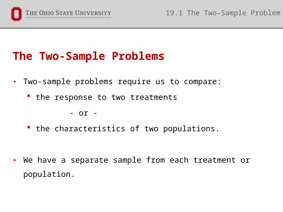
The Two-Sample Problems
▸ Two-sample problems require us to compare:
the response to two treatments
- or -
the characteristics of two populations.
▸ We have a separate sample from each treatment or population.
19.1 The Two-Sample Problem

Two-Sample Problems
▸ The end of Chapter 18 described inference procedures for the mean difference in two measurements on one group of subjects (e.g., pulse rates for 12 students before-and-after listening to music).
▸ Given our answer from above, and the likelihood that each sample has different sample sizes, variances, etc… Chapter 19 focuses on the difference in means for 2 different groups.
PopulationParameter
Point EstimateConfidence
IntervalTest Statistic
19.1 The Two-Sample Problem

Sampling Distribution of Two Sample Means
▸ Recall that for a single sample mean The standard deviation of a statistic is estimated from data the
result is called the standard error of the statistic.
The standard error of is .
▸ Inference in the two-sample problem will require the standard error of the difference of two sample means .
19.2 Comparing Two Population Means

Sampling Distribution of Two Sample Means
▸ The following table stems from the above comment on standard error
and statistical theory.
19.2 Comparing Two Population Means
Variable Parameter Point Estimate PopulationStandard Deviation
Standard Error
x1m1 s1
x2m2 s2
Diff = x1 - x2
m1 - m2
1x2x1x2x
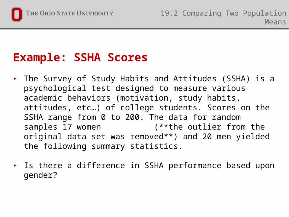
Example: SSHA Scores
▸ The Survey of Study Habits and Attitudes (SSHA) is a psychological test designed to measure various academic behaviors (motivation, study habits, attitudes, etc…) of college students. Scores on the SSHA range from 0 to 200. The data for random samples 17 women (**the outlier from the original data set was removed**) and 20 men yielded the following summary statistics.
▸ Is there a difference in SSHA performance based upon gender?
19.2 Comparing Two Population Means

Example: SSHA Scores
▸ Summary statistics for the two groups are below:
There is a difference in these two groups. The women’s average was 17 points > than the men’s average.
Group Sample Mean
Sample Standard Deviation
Sample Size
Women** 139.588 20.363 17
Men 122.5 32.132 20
19.2 Comparing Two Population Means

Example: SSHA Scores
▸ Summary statistics for the two groups are below:
There is a difference in these two groups. The women’s average was 17 points > than the men’s average.
Yet, the standard deviations are larger than this sample difference, and the sample sizes are about the same.
Is this difference significant enough to conclude that women is different than men?
Group Sample Mean
Sample Standard Deviation
Sample Size
Women** 139.588 20.363 17
Men 122.5 32.132 20
19.2 Comparing Two Population Means

Example: SSHA Scores
▸ Summary statistics for the two groups are below:
There is a difference in these two groups. The women’s average was 17 points > than the men’s average.
Yet, the standard deviations are larger than this sample difference, and the sample sizes are about the same.
Is this difference significant enough to conclude that women is different than men? Let’s
learn more!
Group Sample Mean
Sample Standard Deviation
Sample Size
Women** 139.588 20.363 17
Men 122.5 32.132 20
19.2 Comparing Two Population Means
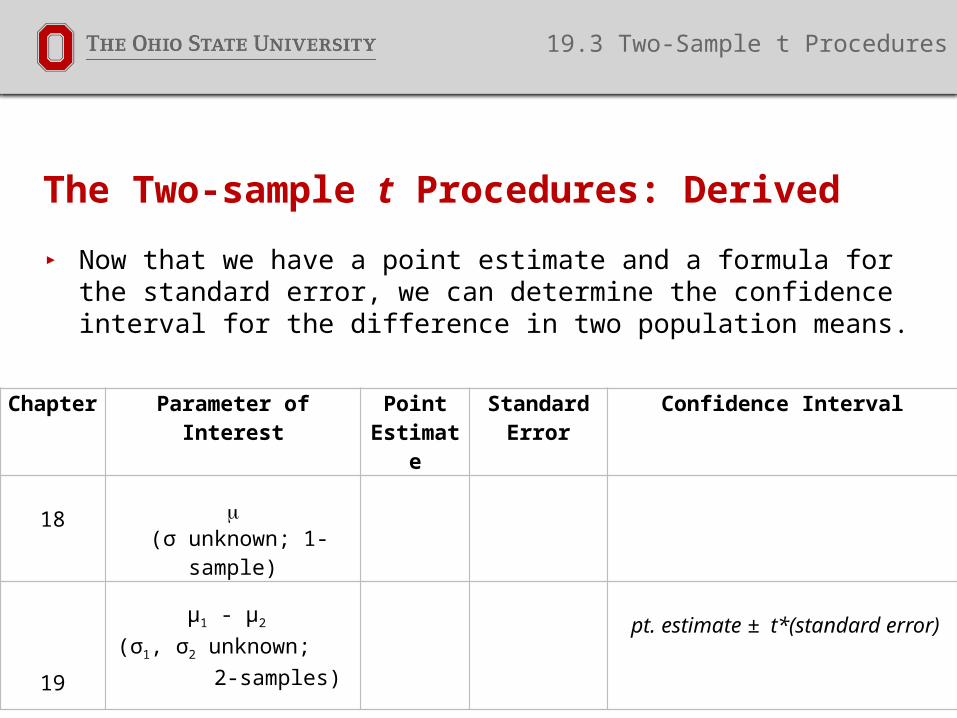
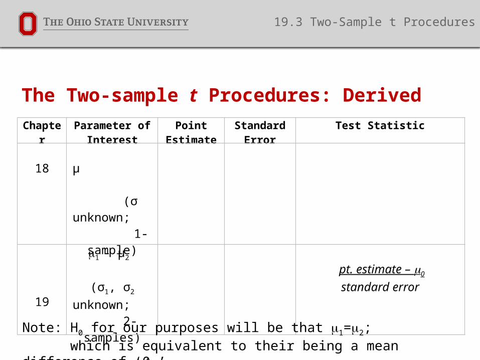
The Two-sample t Procedures: Derived
▸ Now that we have a point estimate and a formula for the standard error, we can determine the confidence interval for the difference in two population means.
Chapter Parameter of Interest Point Estimate
Standard Error
Confidence Interval
18 m (σ unknown; 1-sample)
19
μ1 - μ2 (σ1, σ2 unknown; 2-
samples)
pt. estimate ± t*(standard error)
19.3 Two-Sample t Procedures

The Two-sample t Procedures: Derived
▸ Now that we have a point estimate and a formula for the standard error, we can determine the confidence interval for the difference in two population means.
Chapter Parameter of Interest Point Estimate
Standard Error
Confidence Interval
18 m (σ unknown; 1-sample)
19
μ1 - μ2 (σ1, σ2 unknown; 2-
samples)
pt. estimate ± t*(standard error)
() ± t*
19.3 Two-Sample t Procedures
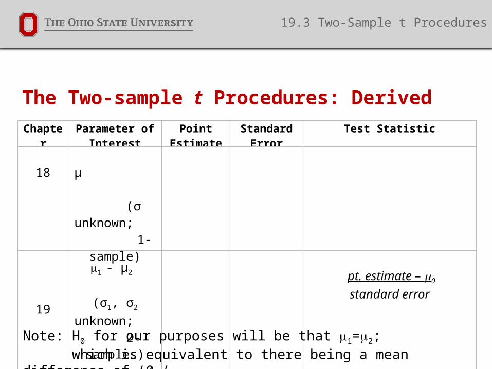
The Two-sample t Procedures: Derived
19.3 Two-Sample t Procedures
Chapter Parameter of Interest
Point Estimate
Standard Error
Test Statistic
18 μ (σ unknown;
1-sample)
19
m1 - μ2
(σ1, σ2 unknown;
2-samples)
pt. estimate – m0
standard error
Note: H0 for our purposes will be that m1=m2; which is equivalent to there being a mean difference of ‘0.’
The Two-sample t Procedures: Derived
19.3 Two-Sample t Procedures
Chapter Parameter of Interest
Point Estimate
Standard Error
Test Statistic
18 μ (σ unknown;
1-sample)
19
m1 - μ2
(σ1, σ2 unknown;
2-samples)
pt. estimate – m0
standard error
Note: H0 for our purposes will be that m1=m2; which is equivalent to their being a mean difference of ‘0.’
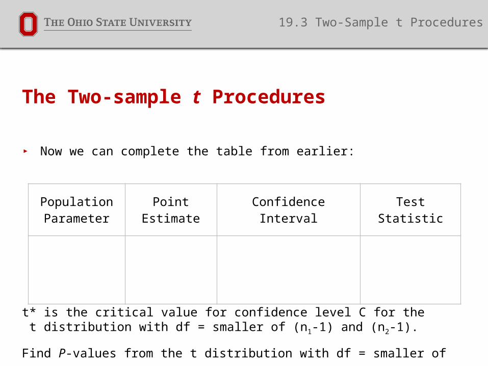
The Two-sample t Procedures
▸ Now we can complete the table from earlier:
t* is the critical value for confidence level C for the t distribution with df = smaller of (n1-1) and (n2-1).
Find P-values from the t distribution with df = smaller of (n1-1) and (n2-1).
PopulationParameter
Point Estimate Confidence Interval Test Statistic
19.3 Two-Sample t Procedures

The Two-sample t Procedures
▸ Now we can complete the table from earlier:
t* is the critical value for confidence level C for the t distribution with df = smaller of (n1-1) and (n2-1).
Find P-values from the t distribution with df = smaller of (n1-1) and (n2-1).
PopulationParameter
Point Estimate Confidence Interval Test Statistic
() ± t*
19.3 Two-Sample t Procedures
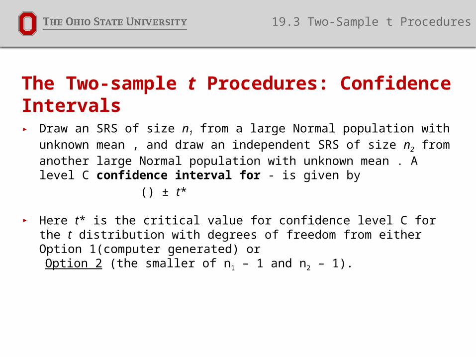
The Two-sample t Procedures: Confidence Intervals▸ Draw an SRS of size n1 from a large Normal population with unknown mean ,
and draw an independent SRS of size n2 from another large Normal population with unknown mean . A level C confidence interval for - is given by
() ± t*
▸ Here t* is the critical value for confidence level C for the t distribution with degrees of freedom from either Option 1(computer generated) or
Option 2 (the smaller of n1 – 1 and n2 – 1).
19.3 Two-Sample t Procedures
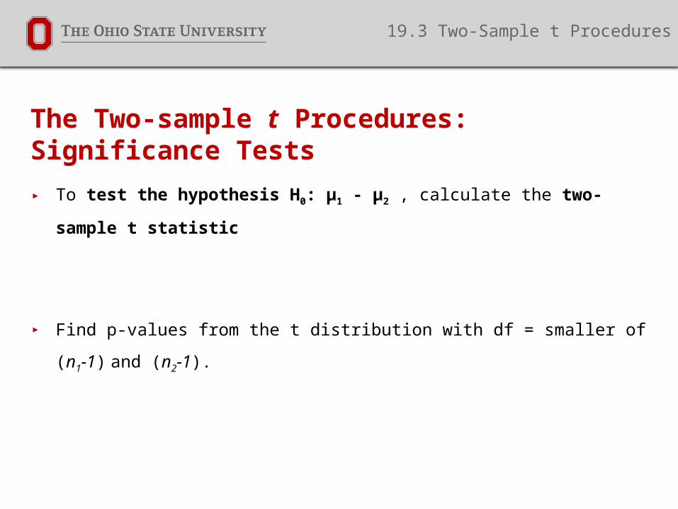
The Two-sample t Procedures: Significance Tests
▸ To test the hypothesis H0: μ1 - μ2 , calculate the two-sample t statistic
▸ Find p-values from the t distribution with df = smaller of (n1-1) and (n2-1).
19.3 Two-Sample t Procedures

Conditions for Inference Comparing Two- Sample Means and Robustness of t Procedures▸ The general structure of our necessary conditions is an extension of
the one-sample cases.
Simple Random Samples:
Do we have 2 simple random samples?
Population : Sample Ratio:
The samples must be independent and from two large populations of
interest.
19.0 Two-Sample Problems
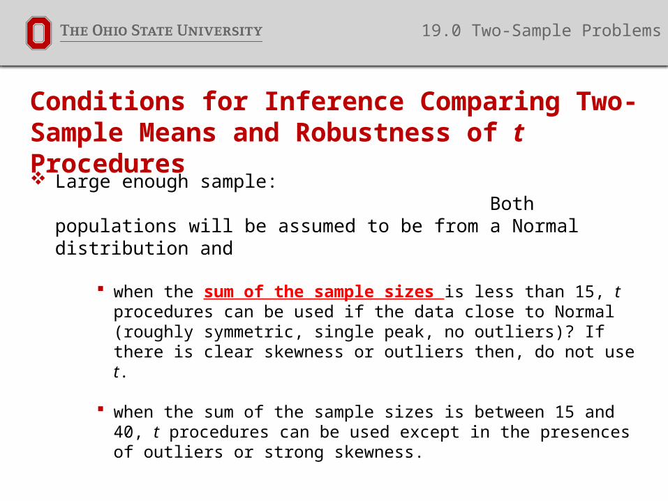
Conditions for Inference Comparing Two- Sample Means and Robustness of t Procedures Large enough sample:
Both populations will be assumed to be from a Normal distribution and
when the sum of the sample sizes is less than 15, t procedures can be used if the data close to Normal (roughly symmetric, single peak, no outliers)? If there is clear skewness or outliers then, do not use t.
when the sum of the sample sizes is between 15 and 40, t procedures can be used except in the presences of outliers or strong skewness.
when the sum of the sample sizes is at least 40, the t procedures can be used even for clearly skewed distributions.
19.0 Two-Sample Problems

Conditions for Inference Comparing Two- Sample Means and Robustness of t Procedures▸ Note: In practice it is enough that the two distributions have similar
shape with no strong outliers. The two-sample t procedures are even more robust against non-Normality than the one-sample procedures.
19.0 Two-Sample Problems

Example: SSHA Scores
▸ The summary statistics for the SSHA scores for random samples of
men and women are below. There was neither significant skewness,
nor, strong outliers, in either data set. Use this information to construct
a 90% confidence interval for the mean difference.
19.3 Two-Sample t Procedures
Group Sample Mean
Sample Standard Deviation
Sample Size
Women 139.588 20.363 17
Men 122.5 32.132 20

Example: 90% CI for SSHA Scores
1. Components Do we have two simple random samples?
Yes. It was stated.
Large enough population: sample ratio? Yes. NW > 20*17 = 340
NM > 20*20 = 400(Independence)
Large enough sample? Yes. nW + nM =37 < 40
but outlier has been removed. No skewness.
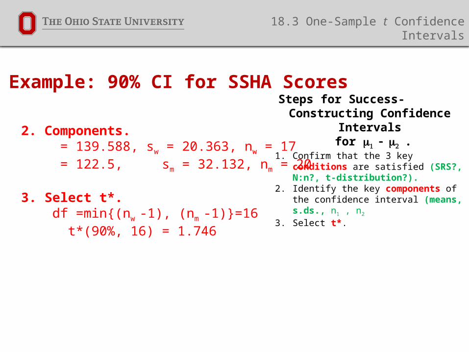
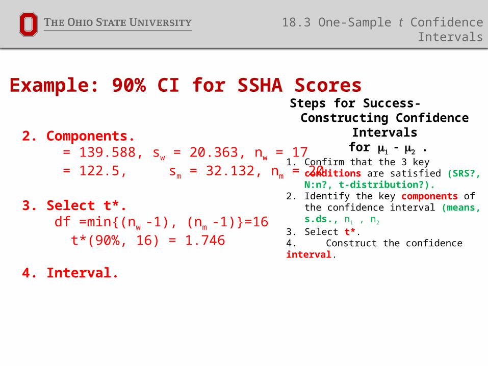
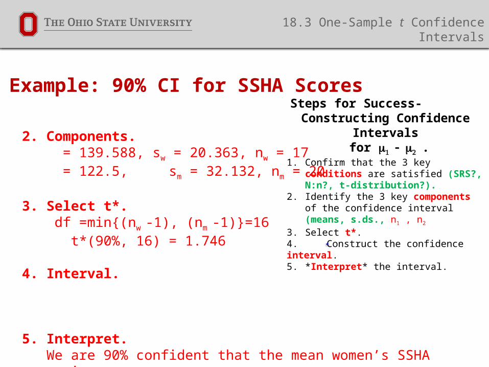
Steps for Success- Constructing Confidence Intervals
for m1 - m2 .1. Confirm that the 3 key conditions are satisfied
(SRS?, N:n?, t-distribution?).
18.3 One-Sample t Confidence Intervals

Example: 90% CI for SSHA Scores Steps for Success-
Constructing Confidence Intervals for m1 - m2 .
1. Confirm that the 3 key conditions are satisfied (SRS?, N:n?, t-distribution?).
2. Identify the key components of the confidence interval (means, s.ds., n1 , n2
18.3 One-Sample t Confidence Intervals

Example: 90% CI for SSHA Scores
2. Components. = 139.588, sw = 20.363, nw = 17 = 122.5, sm = 32.132, nm = 20
Steps for Success- Constructing Confidence Intervals
for m1 - m2 .1. Confirm that the 3 key conditions are satisfied
(SRS?, N:n?, t-distribution?). 2. Identify the key components of the
confidence interval (means, s.ds., n1 , n2
18.3 One-Sample t Confidence Intervals

Example: 90% CI for SSHA Scores
2. Components. = 139.588, sw = 20.363, nw = 17 = 122.5, sm = 32.132, nm = 20
Steps for Success- Constructing Confidence Intervals
for m1 - m2 .1. Confirm that the 3 key conditions are satisfied
(SRS?, N:n?, t-distribution?). 2. Identify the key components of the
confidence interval (means, s.ds., n1 , n2 3. Select t*.
18.3 One-Sample t Confidence Intervals
Example: 90% CI for SSHA Scores
2. Components. = 139.588, sw = 20.363, nw = 17 = 122.5, sm = 32.132, nm = 20
3. Select t*. df =min{(nw -1), (nm -1)}=16 t*(90%, 16) = 1.746
Steps for Success- Constructing Confidence Intervals
for m1 - m2 .1. Confirm that the 3 key conditions are satisfied
(SRS?, N:n?, t-distribution?). 2. Identify the key components of the
confidence interval (means, s.ds., n1 , n2 3. Select t*.
18.3 One-Sample t Confidence Intervals

Example: 90% CI for SSHA Scores
2. Components. = 139.588, sw = 20.363, nw = 17 = 122.5, sm = 32.132, nm = 20
3. Select t*. df =min{(nw -1), (nm -1)}=16 t*(90%, 16) = 1.746
Steps for Success- Constructing Confidence Intervals
for m1 - m2 .1. Confirm that the 3 key conditions are satisfied
(SRS?, N:n?, t-distribution?). 2. Identify the key components of the
confidence interval (means, s.ds., n1 , n2 3. Select t*.4. Construct the confidence interval.
18.3 One-Sample t Confidence Intervals
Example: 90% CI for SSHA Scores
2. Components. = 139.588, sw = 20.363, nw = 17 = 122.5, sm = 32.132, nm = 20
3. Select t*. df =min{(nw -1), (nm -1)}=16 t*(90%, 16) = 1.746
4. Interval.
Steps for Success- Constructing Confidence Intervals
for m1 - m2 .1. Confirm that the 3 key conditions are satisfied
(SRS?, N:n?, t-distribution?). 2. Identify the key components of the
confidence interval (means, s.ds., n1 , n2 3. Select t*.4. Construct the confidence interval.
18.3 One-Sample t Confidence Intervals

Example: 90% CI for SSHA Scores
2. Components. = 139.588, sw = 20.363, nw = 17 = 122.5, sm = 32.132, nm = 20
3. Select t*. df =min{(nw -1), (nm -1)}=16 t*(90%, 16) = 1.746
4. Interval.
Steps for Success- Constructing Confidence Intervals
for m1 - m2 .1. Confirm that the 3 key conditions are satisfied
(SRS?, N:n?, t-distribution?). 2. Identify the key components of the
confidence interval (means, s.ds., n1 , n2 3. Select t*.4. Construct the confidence interval.5. *Interpret* the interval.
18.3 One-Sample t Confidence Intervals
Example: 90% CI for SSHA Scores
2. Components. = 139.588, sw = 20.363, nw = 17 = 122.5, sm = 32.132, nm = 20
3. Select t*. df =min{(nw -1), (nm -1)}=16 t*(90%, 16) = 1.746
4. Interval.
5. Interpret.We are 90% confident that the mean women’s SSHA score is
between 1.866 and 32.31 points higher than men’s.
Steps for Success- Constructing Confidence Intervals
for m1 - m2 .1. Confirm that the 3 key conditions are satisfied
(SRS?, N:n?, t-distribution?). 2. Identify the 3 key components of the
confidence interval (means, s.ds., n1 , n2 3. Select t*.4. Construct the confidence interval.5. *Interpret* the interval.
18.3 One-Sample t Confidence Intervals

Example: SSHA Scores
▸ Let’s continue with this example by now conducting a test of
significance for the mean difference in SSHA by gender at a=0.10.
19.3 Two-Sample t Procedures
Group Sample Mean
Sample Standard Deviation
Sample Size
Women 139.588 20.363 17
Men 122.5 32.132 20
Example: SSHA Scores
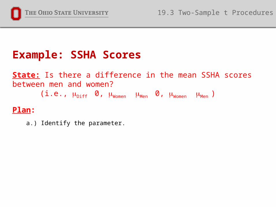
State: Is there a difference in the mean SSHA scores between men and women? (i.e., mDiff 0, mWomen mMen 0, mWomen mMen )
Plan:
a.) Identify the parameter.
19.3 Two-Sample t Procedures

Example: SSHA Scores
State: Is there a difference in the mean SSHA scores between men and women? (i.e., mDiff 0, mWomen mMen 0, mWomen mMen )
Plan:
a.) Identify the parameter. mDiff =mWomen - mMen.
b) List all given information from the data collected.
19.3 Two-Sample t Procedures
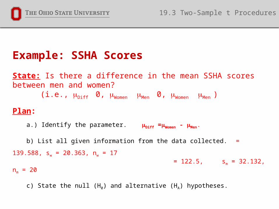
Example: SSHA Scores
State: Is there a difference in the mean SSHA scores between men and women? (i.e., mDiff 0, mWomen mMen 0, mWomen mMen )
Plan:
a.) Identify the parameter. mDiff =mWomen - mMen.
b) List all given information from the data collected. = 139.588, sw = 20.363, nw =
17
= 122.5, sm = 32.132, nm = 20
c) State the null (H0) and alternative (HA) hypotheses.
19.3 Two-Sample t Procedures

Example: SSHA Scores
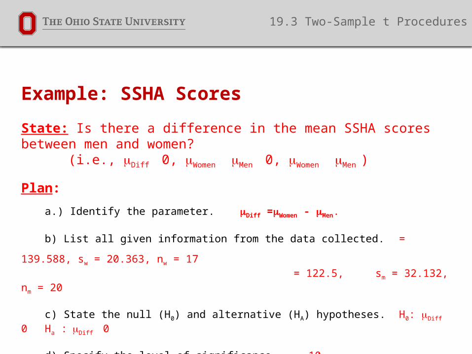
State: Is there a difference in the mean SSHA scores between men and women? (i.e., mDiff 0, mWomen mMen 0, mWomen mMen )
Plan:
a.) Identify the parameter. mDiff =mWomen - mMen.
b) List all given information from the data collected. = 139.588, sw = 20.363, nw =
17
= 122.5, sm = 32.132, nm = 20
c) State the null (H0) and alternative (HA) hypotheses. H0: mDiff 0Ha : mDiff 0
19.3 Two-Sample t Procedures
Example: SSHA Scores
State: Is there a difference in the mean SSHA scores between men and women? (i.e., mDiff 0, mWomen mMen 0, mWomen mMen )
Plan:
a.) Identify the parameter. mDiff =mWomen - mMen.
b) List all given information from the data collected. = 139.588, sw = 20.363, nw =
17
= 122.5, sm = 32.132, nm = 20
c) State the null (H0) and alternative (HA) hypotheses. H0: mDiff 0Ha : mDiff 0
d) Specify the level of significance. a =.10
e) Determine the type of test. Left-tailed Right-tailed Two-
Tailed
19.3 Two-Sample t Procedures

Example: SSHA Scores
Plan:
f) Sketch the region(s) of “extremely unlikely” test statistics.
19.3 Two-Sample t Procedures

Example: SSHA Scores
Solve:
a) Check the conditions for the test you plan to use.
Two Simple Random Samples?
Large enough population: sample ratios?
Large enough samples?
19.3 Two-Sample t Procedures

Example: SSHA Scores
Solve:
a) Check the conditions for the test you plan to use.
Two Simple Random Samples?
Yes. Stated as a random sample.
Large enough population: sample ratios?
Yes. Both populations are arbitrarily large; much greater than, NW > 20*17 = 340; NM > 20*20
= 400
Large enough samples?
Yes. nW + nM =37 < 40 outlier has been removed. No skewness.
19.3 Two-Sample t Procedures

Example: SSHA Scores
Solve:
b) Calculate the test statistic
c) Determine (or approximate) the P-Value.
t =
19.3 Two-Sample t Procedures
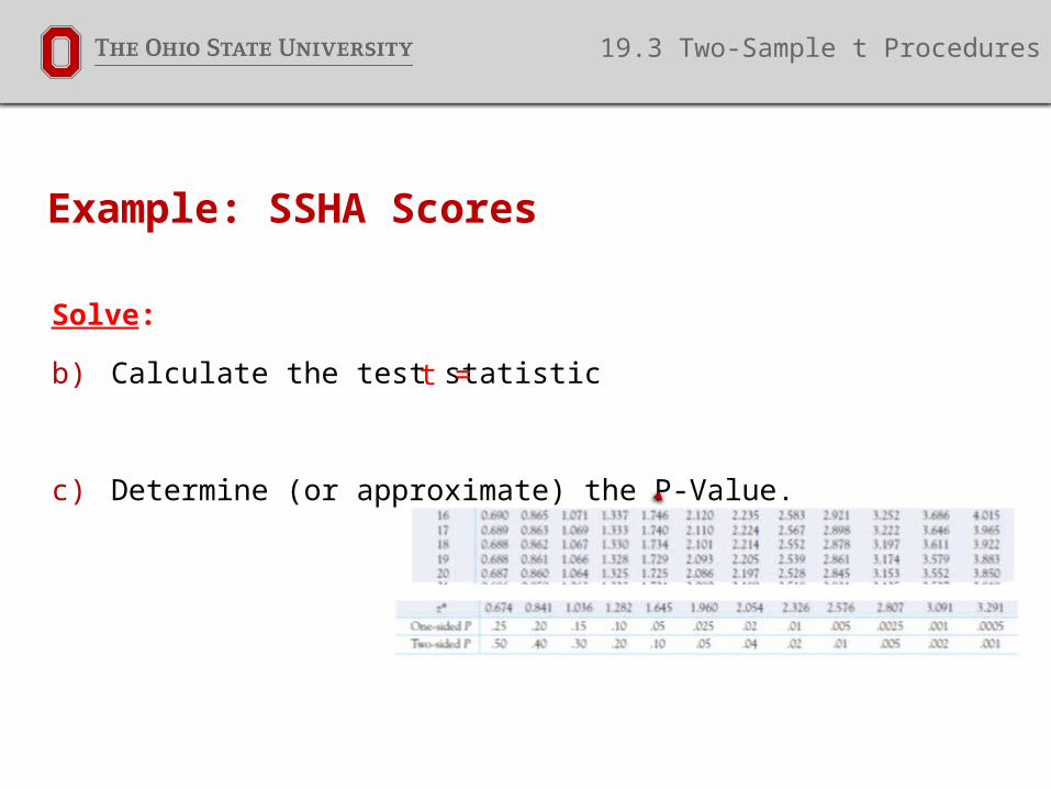
Example: SSHA Scores
Solve:
b) Calculate the test statistic
c) Determine (or approximate) the P-Value.
t =
19.3 Two-Sample t Procedures
Example: SSHA Scores
Solve:
b) Calculate the test statistic
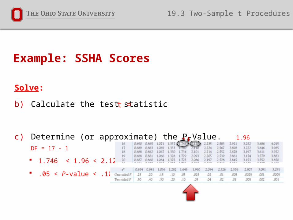
c) Determine (or approximate) the P-Value. 1.96 DF = 17 - 1
1.746 < 1.96 < 2.12
.05 < P-value < .10
P-value
t =
19.3 Two-Sample t Procedures

Example: SSHA Scores
Conclude: a) Make a decision about the null hypothesis (Reject H0 or Fail to reject H0).
19.3 Two-Sample t Procedures

Example: SSHA Scores
Conclude: a) Make a decision about the null hypothesis (Reject H0 or Fail to reject H0).
Because the approximate P-value is smaller than 0.10, we reject the null hypothesis.
b) Interpret the decision in the context of the original claim.
19.3 Two-Sample t Procedures

Example: SSHA Scores
Conclude: a) Make a decision about the null hypothesis (Reject H0 or Fail to reject H0).
Because the approximate P-value is smaller than 0.10, we reject the null hypothesis.
b) Interpret the decision in the context of the original claim.There is enough evidence (at a=.10)
that there is a difference in the mean SSHA score between men and women.
19.3 Two-Sample t Procedures
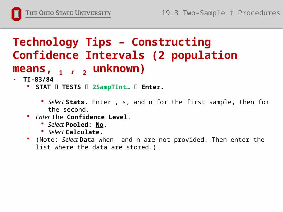
Technology Tips – Constructing Confidence Intervals (2 population means, 1 , 2 unknown)
▸ TI-83/84 STAT TESTS 2SampTInt… Enter.
Select Stats. Enter , s, and n for the first sample, then for the second.
Enter the Confidence Level. Select Pooled: No. Select Calculate.
(Note: Select Data when and n are not provided. Then enter the list where the data are stored.)
19.3 Two-Sample t Procedures

Technology Tips – Constructing Confidence Intervals (2 population means, 1 , 2 unknown)
▸ JMP Enter the quantitative data into one of the columns. In the next column, enter an abridged description of the categorical variable
associated with each row of quantitative data. (Note: Pay attention to the spelling and capitalization of the abridged descriptions.)
Analyze Fit Y by X. “Click-and-Drag” (the quantitative variable) into the ‘Y, Response’ box. “Click-and-
Drag” (the categorical variable) into the ‘X, Factor’ box. Click on OK. Click on the red upside-down triangle next to the title “Oneway Analysis of …”
Proceed to ‘Means and Std Dev.’
Click on the red upside-down triangle next to the title “Oneway Analysis of …”
Proceed to ‘t Test.’
19.3 Two-Sample t Procedures

Technology Tips – Significance Tests (2 population means, 1 , 2 unknown)
▸ TI-83/84
STAT TESTS 2SampTTest Enter.
Select Stats. Enter , s, and n for the first sample, then for the second.
(Note: Select Data when and n are not provided. Then enter the list where
the data are stored.)
Select the inequality that corresponds to the alternative hypothesis.
Select Pooled: No.
Select Calculate.
19.3 Two-Sample t Procedures

Technology Tips – Significance Tests (2 population means, 1 , 2 unknown)▸ JMP
Enter the quantitative data into one of the columns.
In the next column, enter an abridged description of the categorical variable associated with
each row of quantitative data.
▸ (Note: Pay attention to the spelling and capitalization of the abridged descriptions.)
Analyze Fit Y by X.
“Click-and-Drag” (the quantitative variable) into the ‘Y, Response’ box.
“Click-and-Drag” (the categorical variable) into the ‘X, Factor’ box. Click on OK.
Click on the red upside-down triangle next to the title “Oneway Analysis of …”
Proceed to ‘Means and Std Dev.’
Click on the red upside-down triangle next to the title “Oneway Analysis of …”
Proceed to ‘t Test.’
19.3 Two-Sample t Procedures
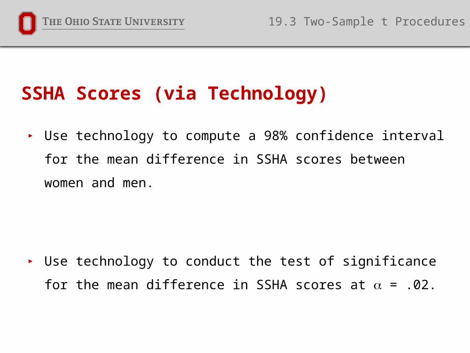
SSHA Scores (via Technology)
▸ Use technology to compute a 98% confidence interval for the mean
difference in SSHA scores between women and men.
▸ Use technology to conduct the test of significance for the mean
difference in SSHA scores at a = .02.
19.3 Two-Sample t Procedures

98% confidence interval for the mean difference in SSHA scores between women & men.
▸ TI-83/84
STAT >> TESTS >> 2SampTInt… >> Enter
Note: Select Data when and are not provided. Then
enter the list where the data are stored.
(for this example)
Inpt >> STATS
1:139.588 >> sx1: 20.363 >> n1: 17 2:122.5 >> sx1: 32.13 >> n1: 20
C-Level : 98
Pooled : No
Calculate (ENTER)
19.3 Two-Sample t Procedures

98% confidence interval for the mean difference in SSHA scores between women & men.
▸ TI-83/84
STAT >> TESTS >> 2SampTInt… >> Enter
Note: Select Data when and are not provided. Then
enter the list where the data are stored.
(for this example)
Inpt >> STATS
1:139.588 >> sx1: 20.363 >> n1: 17 2:122.5 >> sx2: 32.13 >> n2: 20
C-Level : 98
Pooled : No
Calculate (ENTER) ( -4.241, 38.417)
19.3 Two-Sample t Procedures
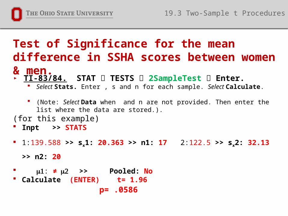
Test of Significance for the mean difference in SSHA scores between women & men.▸ TI-83/84. STAT TESTS 2SampleTest Enter.
Select Stats. Enter , s and n for each sample. Select Calculate. (Note: Select Data when and n are not provided. Then enter the list where the data
are stored.).
(for this example) Inpt >> STATS
1:139.588 >> sx1: 20.363 >> n1: 17 2:122.5 >> sx2: 32.13 >> n2: 20
1m : ≠ 2 m >> Pooled: No Calculate (ENTER) t= 1.96
p= .0586
19.3 Two-Sample t Procedures
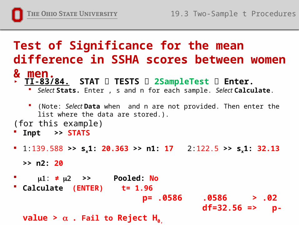
Test of Significance for the mean difference in SSHA scores between women & men.▸ TI-83/84. STAT TESTS 2SampleTest Enter.
Select Stats. Enter , s and n for each sample. Select Calculate. (Note: Select Data when and n are not provided. Then enter the list where the data
are stored.).
(for this example) Inpt >> STATS
1:139.588 >> sx1: 20.363 >> n1: 17 2:122.5 >> sx1: 32.13 >> n2: 20
1m : ≠ 2 m >> Pooled: No Calculate (ENTER) t= 1.96
p= .0586 .0586 > .02
df=32.56 => p-value > a . Fail to Reject H0,
There is not enough evidence (at a = .02) that there is a significant difference in SSHA scores between men and
women. (Note: we did have enough evidence at a = .10).
19.3 Two-Sample t Procedures

Example: SSHA Scores
▸ Technology output for Two Sample Means:
JMP output for the Two-Sample Means’ test of significance and and confidence interval: Means and Std Deviations
Level Number Mean Std Dev Std Err Mean Lower 95% Upper 95% Men 20 122.500 32.1321 7.1850 107.46 137.54 Women 17 139.588 20.3625 4.9386 129.12 150.06
t Test of SSHA by Gender (women – men)
60
80
100
120
140
160
180
200
SSHA
m w
Gender
-30 -20 -10 0 10 20 30
Difference 17.088 t Ratio 1.959977
Std Err Dif 8.719 DF 32.56308
Upper CL Dif 34.835 Prob > |t| 0.0586
Lower CL Dif -0.659 Prob > t 0.0293*
Confidence 0.95 Prob < t 0.9707
19.3 Two-Sample t Procedures

Closing Caveats and Comments
▸ The two-sample t statistic has an approximate (but accurate) t
distribution. The approximate distribution of the two-sample t has an
elaborate degrees of freedom computation (p.480). Computers use
this formula in determining degrees of freedom.
▸ We will use Option 2 (p.470). This has df= smaller of (n1-1) and (n2-1).
▸ Because of the above fact, output in JMP (or other software packages)
might have different df and p-values from manual analyses.
19.3 Two-Sample t Procedures
Closing Caveats and Comments
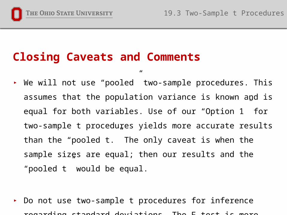
▸ We will not use “pooled” two-sample procedures. This assumes that
the population variance is known and is equal for both variables. Use
of our “Option 1” for two-sample t procedures yields more accurate
results than the “pooled t.” The only caveat is when the sample sizes
are equal; then our results and the “pooled t” would be equal.
▸ Do not use two-sample t procedures for inference regarding standard
deviations. The F-test is more appropriate in those cases.
19.3 Two-Sample t Procedures

Closing Caveats and Comments
▸ Practitioners prefer having equal sample sizes for the two groups when
possible.
▸ Exercises for this chapter will all assume that the SRS is from a
Normal distribution.
19.3 Two-Sample t Procedures

Five-Minute Summary
▸ List at least 3 concepts that had the most impact on your knowledge of
two-sample problems.
_______________ ______________
____________