chapter 17:image post processing and analysis · iaea chapter 17 table of contents 17.1....
TRANSCRIPT

IAEAInternational Atomic Energy Agency
Slide set of 176 slides based on the chapter authored by
P.A. Yushkevich
of the IAEA publication (ISBN 978-92-0-131010-1):
Diagnostic Radiology Physics:
A Handbook for Teachers and Students
Objective:
To familiarize the student with the most common problems in
image post processing and analysis, and the algorithms to
address them.
Chapter 17: Image Post Processing and
Analysis
Slide set prepared
by E. Berry (Leeds, UK and
The Open University in
London)

IAEA
CHAPTER 17 TABLE OF CONTENTS
17.1. Introduction
17.2. Deterministic Image Processing and Feature Enhancement
17.3. Image Segmentation
17.4. Image Registration
17.5. Open-source tools for image analysis
Diagnostic Radiology Physics: A Handbook for Teachers and Students – 17. Slide 1 (02/176)

IAEA
17.1 INTRODUCTION17.1
Diagnostic Radiology Physics: A Handbook for Teachers and Students – 17.1 Slide 1 (03/176)

IAEA
17.1 INTRODUCTION17.1
Introduction (1 of 2)
For decades, scientists have used computers to enhance
and analyze medical images
Initially simple computer algorithms were used to enhance
the appearance of interesting features in images, helping
humans read and interpret them better
Later, more advanced algorithms were developed, where
the computer would not only enhance images, but also
participate in understanding their content
Diagnostic Radiology Physics: A Handbook for Teachers and Students – 17.1 Slide 2 (04/176)
IAEA
17.1 INTRODUCTION17.1
Introduction (2 of 2)
Segmentation algorithms were developed to detect and extract
specific anatomical objects in images, such as malignant lesions in
mammograms
Registration algorithms were developed to align images of different
modalities and to find corresponding anatomical locations in images
from different subjects
These algorithms have made computer-aided detection and diagnosis,
computer-guided surgery, and other highly complex medical
technologies possible
Today, the field of image processing and analysis is a complex branch
of science that lies at the intersection of applied mathematics,
computer science, physics, statistics, and biomedical sciences
Diagnostic Radiology Physics: A Handbook for Teachers and Students – 17.1 Slide 3 (05/176)

IAEA
17.1 INTRODUCTION17.1
Overview
This chapter is divided into two main sections
• classical image processing algorithms
• image filtering, noise reduction, and edge/feature extraction
from images.
• more modern image analysis approaches
• including segmentation and registration
Diagnostic Radiology Physics: A Handbook for Teachers and Students – 17.1 Slide 4 (06/176)

IAEA
17.1 INTRODUCTION17.1
Image processing vs. Image analysis
The main feature that distinguishes image analysis from
image processing is the use of external knowledge about
the objects appearing in the image
This external knowledge can be based on
• heuristic knowledge
• physical models
• data obtained from previous analysis of similar images
Image analysis algorithms use this external knowledge to
fill in the information that is otherwise missing or
ambiguous in the images
Diagnostic Radiology Physics: A Handbook for Teachers and Students – 17.1 Slide 5 (07/176)

IAEA
17.1 INTRODUCTION17.1
Example of image analysis
A biomechanical model of the heart may be used by an
image analysis algorithm to help find the boundaries of the
heart in a CT or MR image
This model can help the algorithm tell true heart
boundaries from various other anatomical boundaries that
have similar appearance in the image
Diagnostic Radiology Physics: A Handbook for Teachers and Students – 17.1 Slide 6 (08/176)

IAEA
17.1 INTRODUCTION17.1
The most important limitation of image processing
Image processing cannot increase the amount of
information available in the input image
Applying mathematical operations to images can only
remove information present in an image
• sometimes, removing information that is not relevant can make it
easier for humans to understand images
Image processing is always limited by the quality of the
input data
• if an imaging system provides data of unacceptable quality, it is
better to try to improve the imaging system, rather than hope that
the “magic” of image processing will compensate for poor imaging
Diagnostic Radiology Physics: A Handbook for Teachers and Students – 17.1 Slide 7 (09/176)
IAEA
17.1 INTRODUCTION17.1
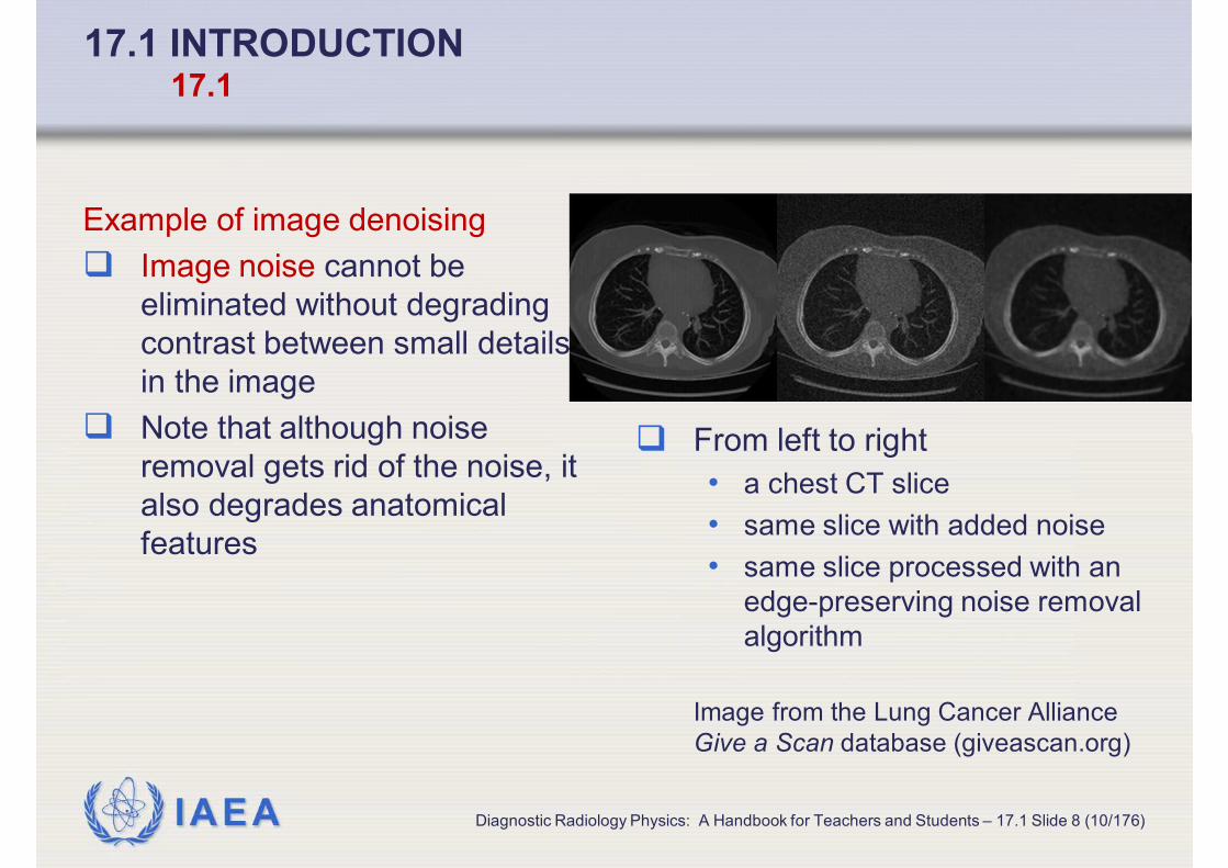
Example of image denoising
Image noise cannot be
eliminated without degrading
contrast between small details
in the image
Note that although noise
removal gets rid of the noise, it
also degrades anatomical
features
From left to right
• a chest CT slice
• same slice with added noise
• same slice processed with an
edge-preserving noise removal
algorithm
Image from the Lung Cancer Alliance
Give a Scan database (giveascan.org)
Diagnostic Radiology Physics: A Handbook for Teachers and Students – 17.1 Slide 8 (10/176)

IAEA
17.1 INTRODUCTION17.1
Changing resolution of an image
The fundamental resolution of
the input image (i.e. the ability
to separate a pair of nearby
structures) is limited by the
imaging system and cannot be
improved by image processing
• in centre image, the system’s
resolution is less than the distance
between the impulses - we cannot
tell from the image that there were
two impulses in the data.
• in the processed image at right we
still cannot tell that there were two
impulses in the input data
From left to right
• the input to an imaging system,
it consists of two nearby point
impulses
• a 16x16 image produced by
the imaging system
• image resampled to 128x128
resolution using cubic
interpolation
Diagnostic Radiology Physics: A Handbook for Teachers and Students – 17.1 Slide 9 (11/176)

IAEA
17.2 DETERMINISTIC IMAGE PROCESSING
AND FEATURE ENHANCEMENT17.2
Diagnostic Radiology Physics: A Handbook for Teachers and Students – 17.2 Slide 1 (12/176)
IAEA
17.2 DETERMINISTIC IMAGE PROCESSING
AND FEATURE ENHANCEMENT17.2.1 SPATIAL FILTERING AND NOISE REMOVAL
Diagnostic Radiology Physics: A Handbook for Teachers and Students – 17.2.1 Slide 1 (13/176)

IAEA
17.2 DETERMINISTIC IMAGE PROCESSING AND
FEATURE ENHANCEMENT 17.2.1 Spatial Filtering and Noise Removal
Filtering
Filtering is an operation that changes the observable
quality of an image, in terms of
• resolution
• contrast
• noise
Typically, filtering involves applying the same or similar
mathematical operation at every pixel in an image
• for example, spatial filtering modifies the intensity of each pixel in
an image using some function of the neighbouring pixels
Filtering is one of the most elementary image processing
operations
Diagnostic Radiology Physics: A Handbook for Teachers and Students – 17.2.1 Slide 2 (14/176)

IAEA
17.2 DETERMINISTIC IMAGE PROCESSING AND
FEATURE ENHANCEMENT 17.2.1 Spatial Filtering and Noise Removal
Mean filtering in the image domain
A very simple example of a spatial filter is the mean filter
Replaces each pixel in an image with the mean of the N x
N neighbourhood around the pixel
The output of the filter is an image that appears more
“smooth” and less “noisy” than the input image
Averaging over the small neighbourhood reduces the
magnitude of the intensity discontinuities in the image
Diagnostic Radiology Physics: A Handbook for Teachers and Students – 17.2.1 Slide 3 (15/176)
Input image convolved
with a 7x7 mean filterInput X ray image

IAEA
17.2 DETERMINISTIC IMAGE PROCESSING AND
FEATURE ENHANCEMENT 17.2.1 Spatial Filtering and Noise Removal
Mean filtering
Mathematically, the mean filter is defined as a convolution
between the image and a constant-valued N x N matrix
The N x N mean filter is a low-pass filter
A low-pass filter reduces high-frequency components in
the Fourier transform (FT) of the image
Diagnostic Radiology Physics: A Handbook for Teachers and Students – 17.2.1 Slide 4 (16/176)
filtered 2
1 1 1
1 1 11;
1 1 1
I I K KN
= =
L
Lo
M M O M
L

IAEA
17.2 DETERMINISTIC IMAGE PROCESSING AND
FEATURE ENHANCEMENT 17.2.1 Spatial Filtering and Noise Removal
Convolution and the Fourier transform
The relationship between Fourier transform (FT) and
convolution is
Convolution of a digital image with a matrix of constant
values is the discrete equivalent of the convolution of a
continuous image function with the rect (boxcar) function
The FT of the rect function is the sinc function
So, mean filtering is equivalent to multiplying the FT of the
image by the sinc function
• this mostly preserves the low-frequency components of the image
and diminishes the high-frequency components
Diagnostic Radiology Physics: A Handbook for Teachers and Students – 17.2.1 Slide 5 (17/176)
F A B F A F B .=o
IAEA
17.2 DETERMINISTIC IMAGE PROCESSING AND
FEATURE ENHANCEMENT 17.2.1 Spatial Filtering and Noise Removal
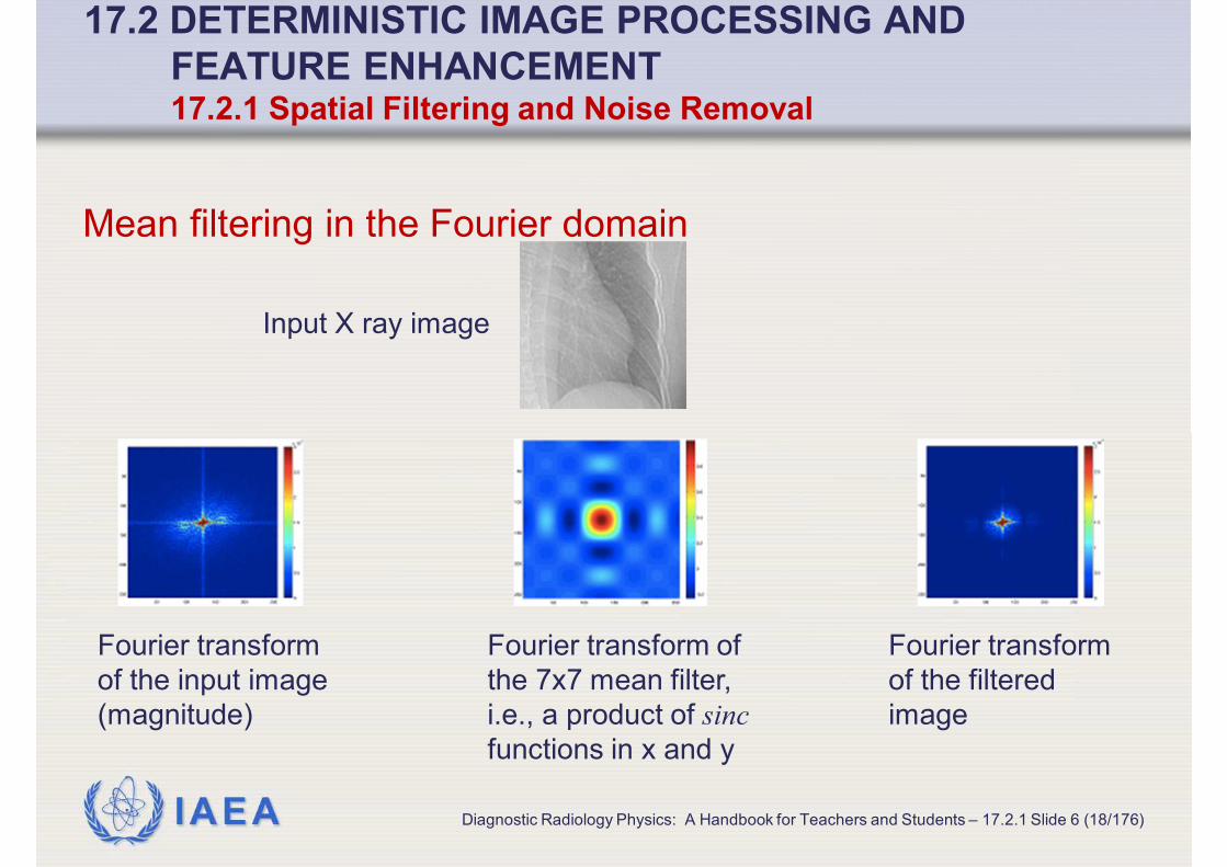
Mean filtering in the Fourier domain
Diagnostic Radiology Physics: A Handbook for Teachers and Students – 17.2.1 Slide 6 (18/176)
Fourier transform of
the 7x7 mean filter,
i.e., a product of sinc
functions in x and y
Input X ray image
Fourier transform
of the input image
(magnitude)
Fourier transform
of the filtered
image
IAEA
17.2 DETERMINISTIC IMAGE PROCESSING AND
FEATURE ENHANCEMENT 17.2.1 Spatial Filtering and Noise Removal
Image smoothing
Mean filtering is an example of an image smoothing
operation
Smoothing and removal of high-frequency noise can help
human observers understand medical images
Smoothing is also an important intermediate step for
advanced image analysis algorithms
Modern image analysis algorithms involve numerical
optimization and require computation of derivatives of
functions derived from image data
• smoothing helps make derivative computation numerically stable
Diagnostic Radiology Physics: A Handbook for Teachers and Students – 17.2.1 Slide 7 (19/176)
IAEA
17.2 DETERMINISTIC IMAGE PROCESSING AND
FEATURE ENHANCEMENT 17.2.1 Spatial Filtering and Noise Removal
Ideal Low-Pass Filter
The so-called ideal low-pass filter cuts off all frequencies above a
certain threshold in the FT of the image
• in the Fourier domain, this is achieved by multiplying the FT of the image
by a cylinder-shaped filter generated by rotating a one-dimensional rect
function around the origin
• theoretically, the same effect is accomplished in the image domain by
convolution with a one-dimensional sinc function rotated around the origin
Assumes that images are periodic functions on an infinite domain
• in practice, most images are not periodic
• convolution with the rotated sinc function results in an artefact called
ringing
Another drawback of the ideal low-pass filter is the computational cost,
which is very high in comparison to mean filtering
Diagnostic Radiology Physics: A Handbook for Teachers and Students – 17.2.1 Slide 8 (20/176)

IAEA
17.2 DETERMINISTIC IMAGE PROCESSING AND
FEATURE ENHANCEMENT 17.2.1 Spatial Filtering and Noise Removal
Ideal low-pass filter and ringing artefact
Diagnostic Radiology Physics: A Handbook for Teachers and Students – 17.2.1 Slide 9 (21/176)
The ideal low-pass filter, i.e.,
a sinc function rotated around
the centre of the image
The original image The image after
convolution with the low-
pass filter. Notice how the
bright intensity of the rib
bones on the right of the
image is replicated in the
soft tissue to the right

IAEA
17.2 DETERMINISTIC IMAGE PROCESSING AND
FEATURE ENHANCEMENT 17.2.1 Spatial Filtering and Noise Removal
Gaussian Filtering
The Gaussian filter is a low-pass filter that is not affected
by the ringing artefact
In the continuous domain, the Gaussian filter is defined as
the normal probability density function with standard
deviation σ, which has been rotated about the origin in x,y
space
Formally, the Gaussian filter is defined as
where the value σ is called the width of the Gaussian filter
Diagnostic Radiology Physics: A Handbook for Teachers and Students – 17.2.1 Slide 10 (22/176)
2 2
222
1( , )
2
x y
G x y e σσ πσ
+−
=

IAEA
17.2 DETERMINISTIC IMAGE PROCESSING AND
FEATURE ENHANCEMENT 17.2.1 Spatial Filtering and Noise Removal
FT of Gaussian filter
The FT of the Gaussian filter is also a Gaussian filter with
reciprocal width 1/σ
where η,υ are spatial frequencies
Diagnostic Radiology Physics: A Handbook for Teachers and Students – 17.2.1 Slide 11 (23/176)
( ) 1/( , ) ( , )F G x y Gσ σ η ν=

IAEA
17.2 DETERMINISTIC IMAGE PROCESSING AND
FEATURE ENHANCEMENT 17.2.1 Spatial Filtering and Noise Removal
Discrete Gaussian filter
The discrete Gaussian filter is a matrix
Its elements, Gij, are given by
The size of the matrix, 2N+1, determines how accurately
the discrete Gaussian approximates the continuous
Gaussian
A common choice is
Diagnostic Radiology Physics: A Handbook for Teachers and Students – 17.2.1 Slide 12 (24/176)
(2 1) (2 1)N N+ × +
( 1, 1)ijG G i N j Nσ= − − − −
3N σ>=

IAEA
17.2 DETERMINISTIC IMAGE PROCESSING AND
FEATURE ENHANCEMENT 17.2.1 Spatial Filtering and Noise Removal
Examples of Gaussian filters
Diagnostic Radiology Physics: A Handbook for Teachers and Students – 17.2.1 Slide 13 (25/176)
A continuous 2D Gaussian
with σ = 2
A discrete 21x21
Gaussian filter with σ = 2

IAEA
17.2 DETERMINISTIC IMAGE PROCESSING AND
FEATURE ENHANCEMENT 17.2.1 Spatial Filtering and Noise Removal
Application of the Gaussian filter
To apply low-pass filtering to a digital image, we
• perform convolution between the image and the Gaussian filter
• this is equivalent to multiplying the FT of the image by a Gaussian filter
with width 1/σ
The Gaussian function decreases very quickly as we move away from
the peak
• at the distance 4σ from the peak, the value of the Gaussian is only 0.0003
of the value at the peak
Convolution with the Gaussian filter
• removes high frequencies in the image
• low frequencies are mostly retained
• the larger the standard deviation of the Gaussian filter, the smoother the
result of the filtering
Diagnostic Radiology Physics: A Handbook for Teachers and Students – 17.2.1 Slide 14 (26/176)

IAEA
17.2 DETERMINISTIC IMAGE PROCESSING AND
FEATURE ENHANCEMENT 17.2.1 Spatial Filtering and Noise Removal
An image convolved with Gaussian filters with different widths
Diagnostic Radiology Physics: A Handbook for Teachers and Students – 17.2.1 Slide 15 (27/176)
Original image σ=1 σ=4 σ=16

IAEA
17.2 DETERMINISTIC IMAGE PROCESSING AND
FEATURE ENHANCEMENT 17.2.1 Spatial Filtering and Noise Removal
Median Filtering
The median filter replaces each pixel in the image with the
median of the pixel values in an N x N neighbourhood
Taking the median of a set of numbers is a non-linear
operation
• therefore, median filtering cannon be represented as convolution
The median filter is useful for removing impulse noise, a
type of noise where some isolated pixels in the image
have very high or very low intensity values
The disadvantage of median filtering is that it can remove
important features, such as thin edges
Diagnostic Radiology Physics: A Handbook for Teachers and Students – 17.2.1 Slide 16 (28/176)

IAEA
17.2 DETERMINISTIC IMAGE PROCESSING AND
FEATURE ENHANCEMENT 17.2.1 Spatial Filtering and Noise Removal
Example of Median Filtering
Diagnostic Radiology Physics: A Handbook for Teachers and Students – 17.2.1 Slide 17 (29/176)
Original image Image degraded by
adding “salt and
pepper” noise. The
intensity of a tenth of
the pixels has been
replaced by 0 or 255
The result of filtering
the degraded image
with a 5x5 mean filter
The result of filtering
with a 5x5 median
filter. Much of the salt
and pepper noise has
been removed – but
some of the fine lines
in the image have
also been removed
by the filtering

IAEA
17.2 DETERMINISTIC IMAGE PROCESSING AND
FEATURE ENHANCEMENT 17.2.1 Spatial Filtering and Noise Removal
Edge-preserving smoothing and de-noising
When we smooth an image, we remove high-frequency
components
This helps reduce noise in the image, but it also can
remove important high-frequency features such as edges
• an edge in image processing is a discontinuity in the intensity
function
• for example, in an X ray image, the intensity is discontinuous along
the boundaries between bone and soft tissue
Some advanced filtering algorithms try to remove noise in
images without smoothing edges
• e.g. the anisotropic diffusion algorithm (Perona and Malik)
Diagnostic Radiology Physics: A Handbook for Teachers and Students – 17.2.1 Slide 18 (30/176)

IAEA
17.2 DETERMINISTIC IMAGE PROCESSING AND
FEATURE ENHANCEMENT 17.2.1 Spatial Filtering and Noise Removal
Anisotropic Diffusion algorithm
Mathematically, smoothing an image with a Gaussian filter is
analogous to simulating heat diffusion in a homogeneous body
In anisotropic diffusion, the image is treated as an inhomogeneous
body, with different heat conductance at different places in the image
• near edges, the conductance is lower, so heat diffuses more slowly,
preventing the edge from being smoothed away
• away from edges, the conductance is faster
The result is that less smoothing is applied near image edges
The approach is only as good as our ability to detect image edges
Diagnostic Radiology Physics: A Handbook for Teachers and Students – 17.2.1 Slide 19 (31/176)
IAEA
17.2 DETERMINISTIC IMAGE PROCESSING
AND FEATURE ENHANCEMENT17.2.2 EDGE, RIDGE AND SIMPLE SHAPE DETECTION
Diagnostic Radiology Physics: A Handbook for Teachers and Students – 17.2.2 Slide 1 (32/176)
IAEA
17.2 DETERMINISTIC IMAGE PROCESSING AND
FEATURE ENHANCEMENT 17.2.2 Edge, Ridge and Simple Shape Detection
Edges
One of the main applications of image processing and
image analysis is to detect structures of interest in images
In many situations, the structure of interest and the
surrounding structures have different image intensities
By searching for discontinuities in the image intensity
function, we can find the boundaries of structures of
interest
• these discontinuities are called edges
• for example, in an X ray image, there is an edge at the boundary
between bone and soft tissue
Diagnostic Radiology Physics: A Handbook for Teachers and Students – 17.2.2 Slide 2 (33/176)

IAEA
17.2 DETERMINISTIC IMAGE PROCESSING AND
FEATURE ENHANCEMENT 17.2.2 Edge, Ridge and Simple Shape Detection
Edge detection
Edge detection algorithms search for edges in images automatically
Because medical images are complex, they have very many
discontinuities in the image intensity
• most of these are not related to the structure of interest
• may be discontinuities due to noise, imaging artefacts, or other structures
Good edge detection algorithms identify edges that are more likely to
be of interest
However, no matter how good an edge detection algorithm is, it will
frequently find irrelevant edges
• edge detection algorithms are not powerful enough to completely
automatically identify structures of interest in most medical images
• instead, they are a helpful tool for more complex segmentation algorithms,
as well as a useful visualization tool
Diagnostic Radiology Physics: A Handbook for Teachers and Students – 17.2.2 Slide 3 (34/176)

IAEA
17.2 DETERMINISTIC IMAGE PROCESSING AND
FEATURE ENHANCEMENT 17.2.2 Edge, Ridge and Simple Shape Detection
Tube detection
Some structures in medical images have very
characteristic shapes
For example, blood vessels are tube-like structures with
• gradually varying width
• two edges that are roughly parallel to each other
This property can be exploited by special tube-detection
algorithms
Diagnostic Radiology Physics: A Handbook for Teachers and Students – 17.2.2 Slide 4 (35/176)

IAEA
17.2 DETERMINISTIC IMAGE PROCESSING AND
FEATURE ENHANCEMENT 17.2.2 Edge, Ridge and Simple Shape Detection
Illustration of edges and tubes in an image
Diagnostic Radiology Physics: A Handbook for Teachers and Students – 17.2.2 Slide 5 (36/176)
Detail from a chest CT image –
The yellow profile crosses an
edge, and the green profile
crosses a tube-like structure
Plot (blue) of image
intensity along the yellow
profile and a plot (red) of
image intensity after
smoothing the input image
with a Gaussian filter with
σ = 1
Plot of image intensity
along the green profile.
Edge and tube detectors
use properties of image
derivative to detect edges
and tube

IAEA
17.2 DETERMINISTIC IMAGE PROCESSING AND
FEATURE ENHANCEMENT 17.2.2 Edge, Ridge and Simple Shape Detection
How image derivatives are computed
An edge is a discontinuity in the image intensity
Therefore, the directional derivative of the image intensity
in the direction orthogonal to the edge must be large, as
seen in the preceding figure
Edge detection algorithms exploit this property
In order to compute derivatives, we require a continuous
function, but an image is just an array of numbers
One solution is to use the finite difference approximation of
the derivative
Diagnostic Radiology Physics: A Handbook for Teachers and Students – 17.2.2 Slide 6 (37/176)

IAEA
17.2 DETERMINISTIC IMAGE PROCESSING AND
FEATURE ENHANCEMENT 17.2.2 Edge, Ridge and Simple Shape Detection
Finite difference approximation in 1D
From the Taylor series expansion, it is easy to derive the
following approximation of the derivative
where
• δ is a real number
• is the error term, involving δ to the power of two and greater
• when δ<< 1 these error terms are very small and can be ignored for
the purpose of approximation
Diagnostic Radiology Physics: A Handbook for Teachers and Students – 17.2.2 Slide 7 (38/176)
2( ) ( )'( ) ( ),
2
f x f xf x O
δ δδ
δ+ − −
= +
( )2δO

IAEA
17.2 DETERMINISTIC IMAGE PROCESSING AND
FEATURE ENHANCEMENT 17.2.2 Edge, Ridge and Simple Shape Detection
Finite difference approximation in 2D (1 of 2)
Likewise, the partial derivatives of a function of two
variables can be approximated as
Diagnostic Radiology Physics: A Handbook for Teachers and Students – 17.2.2 Slide 8 (39/176)
2
2
( , ) ( , )( , )( ),
2
( , ) ( , )( , )( ).
2
x xx
x
y y
y
y
f x y f x yf x yO
x
f x y f x yf x yO
y
δ δδ
δ
δ δδ
δ
+ − −∂= +
∂
+ − −∂= +
∂

IAEA
17.2 DETERMINISTIC IMAGE PROCESSING AND
FEATURE ENHANCEMENT 17.2.2 Edge, Ridge and Simple Shape Detection
Finite difference approximation in 2D (2 of 2)
If we
• treat a digital image as a set of samples from a continuous image
function
• set δx and δy to be equal to the pixel spacing
We can compute approximate image derivatives using
these formulae
However, the error term is relatively high, of the order of 1
pixel width
In practice, derivatives computed using finite difference
formulae are dominated by noise
Diagnostic Radiology Physics: A Handbook for Teachers and Students – 17.2.2 Slide 9 (40/176)

IAEA
17.2 DETERMINISTIC IMAGE PROCESSING AND
FEATURE ENHANCEMENT 17.2.2 Edge, Ridge and Simple Shape Detection
Computing image derivatives by filtering (1 of 3)
There is another, often more effective, approach to
computing image derivatives
We can reconstruct a continuous signal from an image by
convolution with a smooth kernel (such as a Gaussian),
which allows us to take the derivative of the continuous
signal
Diagnostic Radiology Physics: A Handbook for Teachers and Students – 17.2.2 Slide 10 (41/176)

IAEA
17.2 DETERMINISTIC IMAGE PROCESSING AND
FEATURE ENHANCEMENT 17.2.2 Edge, Ridge and Simple Shape Detection
Computing image derivatives by filtering (2 of 3)
In the above, Dv
denotes the directional derivative of a
function in the direction v
One of the most elegant ways to compute image
derivatives arises from the fact that differentiation and
convolution are commutable operations
• both are linear operations, and the order in which they are applied
does not matter
Diagnostic Radiology Physics: A Handbook for Teachers and Students – 17.2.2 Slide 11 (42/176)
( , ) ( )( , );
( )( , ) ( )( , )
f x y I G x y
D f x y D I G x y
=
=v v
o
o

IAEA
17.2 DETERMINISTIC IMAGE PROCESSING AND
FEATURE ENHANCEMENT 17.2.2 Edge, Ridge and Simple Shape Detection
Computing image derivatives by filtering (3 of 3)
Therefore, we can achieve the same effect by computing
the convolution of the image with the derivative of the
smooth kernel
This leads to a very practical and efficient way of
computing derivatives
• create a filter, which is just a matrix that approximates
• compute numerical convolution between this filter and the image
• this is just another example of filtering described earlier
Diagnostic Radiology Physics: A Handbook for Teachers and Students – 17.2.2 Slide 12 (43/176)
( , ) ( )( , )D f x y I D G x y=v v
o
D Gv

IAEA
17.2 DETERMINISTIC IMAGE PROCESSING AND
FEATURE ENHANCEMENT 17.2.2 Edge, Ridge and Simple Shape Detection
Computing image derivatives by Gaussian filtering
Most frequently G is a Gaussian filter
The Gaussian is infinitely differentiable, so it is possibly to
take an image derivative of any order using this approach
The width of the Gaussian is chosen empirically
• the width determines how smooth the interpolation of the digital
image is
• the more smoothing is applied, the less sensitive will the derivative
function be to small local changes in image intensity
• this can help selection between more prominent and less
prominent edges
Diagnostic Radiology Physics: A Handbook for Teachers and Students – 17.2.2 Slide 13 (44/176)

IAEA
17.2 DETERMINISTIC IMAGE PROCESSING AND
FEATURE ENHANCEMENT 17.2.2 Edge, Ridge and Simple Shape Detection
Examples of Gaussian derivative filters
Diagnostic Radiology Physics: A Handbook for Teachers and Students – 17.2.2 Slide 14 (45/176)
First and second partial derivatives in x of
the Gaussian with σ =2
Corresponding 21 × 21 discrete Gaussian
derivative filters

IAEA
17.2 DETERMINISTIC IMAGE PROCESSING AND
FEATURE ENHANCEMENT 17.2.2 Edge, Ridge and Simple Shape Detection
Edge Detectors Based on First Derivative
A popular and simple edge detector is the Sobel operator
To apply this operator, the image is convolved with a pair
of filters
Diagnostic Radiology Physics: A Handbook for Teachers and Students – 17.2.2 Slide 15 (46/176)
1 0 1 1 2 1
2 0 2 ; 0 0 0
1 0 1 1 2 1
x yS S
− = − = − − − −

IAEA
17.2 DETERMINISTIC IMAGE PROCESSING AND
FEATURE ENHANCEMENT 17.2.2 Edge, Ridge and Simple Shape Detection
Sobel operator
It can be shown that this convolution is quite similar to the
finite difference approximation of the partial derivatives of
the image
In fact, the Sobel operator
• approximates the derivative at the given pixel and the two
neighbouring pixels
• computes a weighted average of these three values with weights
(1,2,-1)
This averaging makes the output of the Sobel operator
slightly less sensitive to noise than simple finite differences
Diagnostic Radiology Physics: A Handbook for Teachers and Students – 17.2.2 Slide 16 (47/176)

IAEA
17.2 DETERMINISTIC IMAGE PROCESSING AND
FEATURE ENHANCEMENT 17.2.2 Edge, Ridge and Simple Shape Detection
Illustration of the Sobel operator
The gradient magnitude is high at image edges, but also at isolated
pixels where image intensity varies due to noise
Diagnostic Radiology Physics: A Handbook for Teachers and Students – 17.2.2 Slide 17 (48/176)
Image from the U.S. National Biomedical Imaging Archive Osteoarthritis Initiative (https://imaging.nci.nih.gov/ncia)
MR image of the
knee
Convolution of
the image with
the Sobel x
derivative filter Sx
Convolution of
the image with
the Sobel y
derivative filter Sy
Gradient
magnitude
image
IAEA
17.2 DETERMINISTIC IMAGE PROCESSING AND
FEATURE ENHANCEMENT 17.2.2 Edge, Ridge and Simple Shape Detection
Gradient magnitude image
The last image is the so-called gradient magnitude image, given by
• large values of the gradient magnitude correspond to edges
• low values are regions where intensity is nearly constant
However, there is no absolute value of the gradient magnitude that
distinguishes an edge from non-edge
• for each image, one has to empirically come up with a threshold to apply
to the gradient magnitude image in order to separate the edges of interest
from spurious edges caused by noise and image artefact
This is one of the greatest limitations of edge detection based on first
derivatives
Diagnostic Radiology Physics: A Handbook for Teachers and Students – 17.2.2 Slide 18 (49/176)
2 2( )x yS S+

IAEA
17.2 DETERMINISTIC IMAGE PROCESSING AND
FEATURE ENHANCEMENT 17.2.2 Edge, Ridge and Simple Shape Detection
Convolution with Gaussian derivative filters
Often, the small amount of smoothing performed by the
Sobel operator is not enough to eliminate the edges
associated with image noise
If we are only interested in very strong edges in the image,
we may want to perform additional smoothing
A common alternative to the Sobel filter is to compute the
partial derivatives of the image intensity using convolution
of the image with Gaussian derivative operators
and
Diagnostic Radiology Physics: A Handbook for Teachers and Students – 17.2.2 Slide 19 (50/176)
xD G yD G

IAEA
17.2 DETERMINISTIC IMAGE PROCESSING AND
FEATURE ENHANCEMENT 17.2.2 Edge, Ridge and Simple Shape Detection
Illustration of Gaussian derivative filters
The gradient magnitude is higher at the image edges, but less than for
the Sobel operator at isolated pixels where image intensity varies due
to noise
Diagnostic Radiology Physics: A Handbook for Teachers and Students – 17.2.2 Slide 20 (51/176)
Image from the U.S. National Biomedical Imaging Archive
Osteoarthritis Initiative (https://imaging.nci.nih.gov/ncia)
MR image of the
knee
Convolution of the
image with the
Gaussian x
derivative filter, with
σ=2
Convolution of the
image with the
Gaussian y
derivative filter, with
σ=2
Gradient
magnitude
image

IAEA
17.2 DETERMINISTIC IMAGE PROCESSING AND
FEATURE ENHANCEMENT 17.2.2 Edge, Ridge and Simple Shape Detection
First derivative filters and noise
Of course, too much smoothing can remove important
edges too
Finding the right amount of smoothing is a difficult and
often ill-posed problem
Diagnostic Radiology Physics: A Handbook for Teachers and Students – 17.2.2 Slide 21 (52/176)

IAEA
17.2 DETERMINISTIC IMAGE PROCESSING AND
FEATURE ENHANCEMENT 17.2.2 Edge, Ridge and Simple Shape Detection
Edge Detectors Based on First Derivative
Imagine a particle crossing an edge in a continuous
smooth image F, moving in the direction orthogonal to the
edge (i.e. in the direction of the image gradient)
If we plot the gradient magnitude of the image along the
path of the particle, we see that at the edge, there is a
local maximum of the gradient magnitude
Diagnostic Radiology Physics: A Handbook for Teachers and Students – 17.2.2 Slide 22 (53/176)
IAEA
17.2 DETERMINISTIC IMAGE PROCESSING AND
FEATURE ENHANCEMENT 17.2.2 Edge, Ridge and Simple Shape Detection
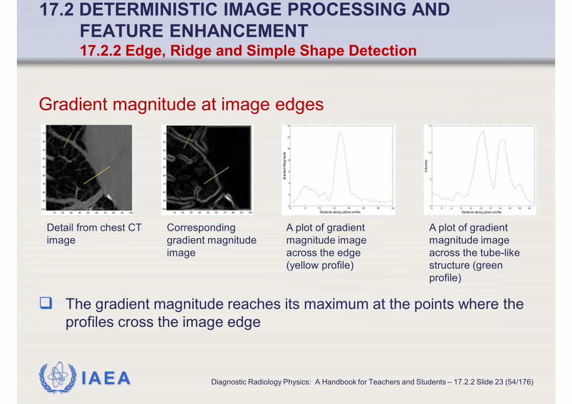
Gradient magnitude at image edges
The gradient magnitude reaches its maximum at the points where the
profiles cross the image edge
Diagnostic Radiology Physics: A Handbook for Teachers and Students – 17.2.2 Slide 23 (54/176)
Detail from chest CT
image
Corresponding
gradient magnitude
image
A plot of gradient
magnitude image
across the edge
(yellow profile)
A plot of gradient
magnitude image
across the tube-like
structure (green
profile)

IAEA
17.2 DETERMINISTIC IMAGE PROCESSING AND
FEATURE ENHANCEMENT 17.2.2 Edge, Ridge and Simple Shape Detection
Local maximum of gradient magnitude
Let us denote the unit vector in the particle’s direction as v,
and the point where the particle crosses the edge as x
The gradient magnitude of the image F at x is simply
The gradient magnitude reaches a local maximum at x in
the direction v if and only if
Several edge detectors leverage this property
Diagnostic Radiology Physics: A Handbook for Teachers and Students – 17.2.2 Slide 24 (55/176)
( ) |F D F∇ =v
x x
0 and 0D F D F= ≤vv vvv

IAEA
17.2 DETERMINISTIC IMAGE PROCESSING AND
FEATURE ENHANCEMENT 17.2.2 Edge, Ridge and Simple Shape Detection
Marr-Hildreth edge detector (1 of 2)
The earliest of these operators is the Marr-Hildreth edge
detector
It is based on the fact that the necessary (but not
sufficient) condition for is
The operator is the Laplacian operator
By finding the set of all points in the image where the
Laplacian of the image is zero, we find the superset of all
the points that satisfy
Diagnostic Radiology Physics: A Handbook for Teachers and Students – 17.2.2 Slide 25 (56/176)
0 and 0D F D F= ≤vv vvv
0xx yyD F D F+ =
xx yyD D+
0 and 0D F D F= ≤vv vvv

IAEA
17.2 DETERMINISTIC IMAGE PROCESSING AND
FEATURE ENHANCEMENT 17.2.2 Edge, Ridge and Simple Shape Detection
Marr-Hildreth edge detector (2 of 2)
When dealing with discrete images, we must use convolution with a
smooth filter (such as the Gaussian) when computing the second
derivatives and the Laplacian
The Marr-Hildreth edge detector convolves the discrete image I with
the Laplacian of Gaussian (LoG) filter:
Next, the Marr-Hildreth edge detector finds contours in the image
where J=0
• these contours are closed and form the superset of edges in the image
The last step is to eliminate the parts of the contour where the gradient
magnitude of the input image is below a user-specified threshold
Diagnostic Radiology Physics: A Handbook for Teachers and Students – 17.2.2 Slide 26 (57/176)
( ) ( ) ( )xx yy xx yyJ I D G D G D I G D I G= + = +o o o

IAEA
17.2 DETERMINISTIC IMAGE PROCESSING AND
FEATURE ENHANCEMENT 17.2.2 Edge, Ridge and Simple Shape Detection
Illustration of Marr-Hildreth edge detector
Diagnostic Radiology Physics: A Handbook for Teachers and Students – 17.2.2 Slide 27 (58/176)
Image from the U.S. National Biomedical Imaging Archive
Osteoarthritis Initiative (https://imaging.nci.nih.gov/ncia)
Input image Zero crossings
of the
convolution of
the image with
the LoG operator
Edges produced by the Marr-
Hildreth detector, i.e., a subset
of the zero crossings that have
gradient magnitude above a
threshold

IAEA
17.2 DETERMINISTIC IMAGE PROCESSING AND
FEATURE ENHANCEMENT 17.2.2 Edge, Ridge and Simple Shape Detection
Canny edge detector
The Canny edge detector is also rooted in the fact that the
second derivative of the image in the edge direction is zero
• applies Gaussian smoothing to the image
• finds the pixels in the image with high gradient magnitude using the
Sobel operator and thresholding
• eliminates pixels that do not satisfy the maximum condition
• uses a procedure called hysteresis to eliminate very short edges
that are most likely the product of noise in the image
The Canny edge detector has very good performance
characteristics compared to other edge detectors
• and is very popular in practice
Diagnostic Radiology Physics: A Handbook for Teachers and Students – 17.2.2 Slide 28 (59/176)
0 and 0D F D F= ≤vv vvv

IAEA
17.2 DETERMINISTIC IMAGE PROCESSING AND
FEATURE ENHANCEMENT 17.2.2 Edge, Ridge and Simple Shape Detection
Illustration of Canny edge detector
Diagnostic Radiology Physics: A Handbook for Teachers and Students – 17.2.2 Slide 29 (60/176)
Image from the U.S. National Biomedical Imaging Archive
Osteoarthritis Initiative (https://imaging.nci.nih.gov/ncia)
Input image Edges produced
by the Sobel
detector
Edges produced
by the Canny
detector

IAEA
17.2 DETERMINISTIC IMAGE PROCESSING AND
FEATURE ENHANCEMENT 17.2.2 Edge, Ridge and Simple Shape Detection
Hough Transform
So far, we have discussed image processing techniques
that search for edges
Sometimes, the objects that we are interested in detecting
have a very characteristic shape: circles, tubes, lines
In these cases, we are better off using detectors that
search for these shapes directly, rather than looking at
edges
The Hough transform is one such detector
Diagnostic Radiology Physics: A Handbook for Teachers and Students – 17.2.2 Slide 30 (61/176)

IAEA
17.2 DETERMINISTIC IMAGE PROCESSING AND
FEATURE ENHANCEMENT 17.2.2 Edge, Ridge and Simple Shape Detection
Hough Transform – simplified
problem (1 of 2)
Given a set of points in
the plane
Find lines, circles or
ellipses approximately
formed by these points
Diagnostic Radiology Physics: A Handbook for Teachers and Students – 17.2.2 Slide 31 (62/176)

IAEA
17.2 DETERMINISTIC IMAGE PROCESSING AND
FEATURE ENHANCEMENT 17.2.2 Edge, Ridge and Simple Shape Detection
Hough Transform – simplified problem (2 of 2)
Simple shapes, like lines, circles and ellipses, can be
described by a small number of parameters
• circles are parameterized by the centre (2 parameters) and radius
(1 parameter)
• ellipses are parameterized by four parameters
• lines are naturally parameterized by the slope and intercept (2
parameters)
• however, this parameterization is asymptotic for vertical lines
• an alternative parameterization by Duda and Hart (1972) uses
the distance from the line to the origin and the slope of the
normal to the line as the two parameters describing a line
Diagnostic Radiology Physics: A Handbook for Teachers and Students – 17.2.2 Slide 32 (63/176)
IAEA
17.2 DETERMINISTIC IMAGE PROCESSING AND
FEATURE ENHANCEMENT 17.2.2 Edge, Ridge and Simple Shape Detection
Hough Transform – parameter space
Each line, circle, or ellipse corresponds to a single point in
the corresponding 2, 3 or 4 dimensional parameter space
The set of all lines, circles, or ellipses passing through a
certain point (x,y) in the image space corresponds to an
infinite set of points in the parameter space
These points in the parameter space form a manifold
For example
• all lines passing through (x,y) form a sinusoid in the Duda and Hart
2-dimensional line parameter space
• all circles passing through (x,y) form a cone in the 3-dimensional
circle parameter space
Diagnostic Radiology Physics: A Handbook for Teachers and Students – 17.2.2 Slide 33 (64/176)

IAEA
17.2 DETERMINISTIC IMAGE PROCESSING AND
FEATURE ENHANCEMENT 17.2.2 Edge, Ridge and Simple Shape Detection
Hough Transform – image domain to parameter domain
This is the meaning of the Hough transform
It transforms points in the image domain into curves,
surfaces or hypersurfaces in the parameter domain
If several points in the image domain belong to a single
line, circle or ellipse, then their corresponding manifolds in
the parameter space intersect at a single point (p1, …, pk)
This gives rise to the shape detection algorithm
Diagnostic Radiology Physics: A Handbook for Teachers and Students – 17.2.2 Slide 34 (65/176)

IAEA
17.2 DETERMINISTIC IMAGE PROCESSING AND
FEATURE ENHANCEMENT 17.2.2 Edge, Ridge and Simple Shape Detection
Hough Transform – shape detection algorithm
The 2, 3 or 4-dimensional parameter space is divided into a finite set
of bins and every bin j is assigned a variable qj that is initialized to zero
For every point (xI,yI) in the image domain
• compute the corresponding curve, surface, or hypersurface in the
parameter space
• find all the bins in the parameter space though which the manifold passes
Every time that the curve, surface or hyper-surface passes through the
bin j
• increment the corresponding variable qj by 1
Once this procedure is completed for all N points
• look for the bins where qj is large
• these bins correspond to a set of qj points that approximately form a line,
circle or ellipse
Diagnostic Radiology Physics: A Handbook for Teachers and Students – 17.2.2 Slide 35 (66/176)

IAEA
17.2 DETERMINISTIC IMAGE PROCESSING AND
FEATURE ENHANCEMENT 17.2.2 Edge, Ridge and Simple Shape Detection
Hough Transform for shape detection
The Hough transform, combined with edge detection, can
be used to search for simple shapes in digital images
• the edge detector is used to find candidate boundary points
• then the Hough transform is used to find simple shapes
The Hough transform is an elegant and efficient approach,
but it scales poorly to more complex objects
• objects more complex than lines, circles, and ellipses require a
large number of parameters to describe them
• the higher the dimensionality of the parameter space, the more
memory- and computationally-intensive the Hough transform
Diagnostic Radiology Physics: A Handbook for Teachers and Students – 17.2.2 Slide 36 (67/176)
1 1( , ) ( , )N Nx y x y…

IAEA
17.2 DETERMINISTIC IMAGE PROCESSING AND
FEATURE ENHANCEMENT 17.2.2 Edge, Ridge and Simple Shape Detection
Illustration of Hough transform
Diagnostic Radiology Physics: A Handbook for Teachers and Students – 17.2.2 Slide 37 (68/176)
An input fluoroscopy
image of a surgical
catheter. The catheter
is almost straight,
making it a good
candidate for detection
with the Hough
transform
Edge map
produced by the
Canny edge
detector
Superimposed Hough
transforms of the edge
points. The Hough
transform of a point in
image space is a sinusoid
in Hough transform space.
The plot shows the number
of sinusoids that pass
through every bin in the
Hough transform space
The lines shown
correspond with
the two bins
through which
many sinusoids
pass
a. b. c. d.
IAEA
17.3 IMAGE SEGMENTATION17.3
Diagnostic Radiology Physics: A Handbook for Teachers and Students – 17.3 Slide 1 (69/176)

IAEA
17.3 IMAGE SEGMENTATION17.3
17.3.1 Object representation
17.3.2 Thresholding
17.3.3 Automatic tissue classification
17.3.4 Active contour segmentation methods
17.3.5 Atlas-based segmentation
Diagnostic Radiology Physics: A Handbook for Teachers and Students – 17.3 Slide 2 (70/176)
IAEA
17.3 IMAGE SEGMENTATION 17.3
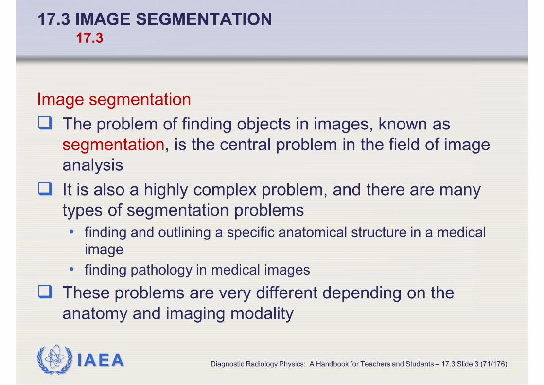
Image segmentation
The problem of finding objects in images, known as
segmentation, is the central problem in the field of image
analysis
It is also a highly complex problem, and there are many
types of segmentation problems
• finding and outlining a specific anatomical structure in a medical
image
• finding pathology in medical images
These problems are very different depending on the
anatomy and imaging modality
Diagnostic Radiology Physics: A Handbook for Teachers and Students – 17.3 Slide 3 (71/176)

IAEA
17.3 IMAGE SEGMENTATION 17.3
Challenges of image segmentation
Heart segmentation in CT is very different from heart segmentation in
MRI, which is very different from brain segmentation in MRI
Some structures move during imaging, while other structures are
almost still
Some structures have a simple shape that varies little from subject to
subject, while others have complex, unpredictable shapes
Some structures have good contrast with surrounding tissues, and
others do not
More often than not, a given combination of anatomical structure and
imaging modality requires a custom segmentation algorithm
Diagnostic Radiology Physics: A Handbook for Teachers and Students – 17.3 Slide 4 (72/176)

IAEA
17.3 IMAGE SEGMENTATION17.3.1 OBJECT REPRESENTATION
Diagnostic Radiology Physics: A Handbook for Teachers and Students – 17.3.1 Slide 1 (73/176)

IAEA
17.3 IMAGE SEGMENTATION 17.3.1 Object Representation
Methods of representing objects in images
Binary image or label image
Geometric boundary representations
Level sets of real-valued images
Several other representations are available, but they are
not discussed here
Diagnostic Radiology Physics: A Handbook for Teachers and Students – 17.3.1 Slide 2 (74/176)

IAEA
17.3 IMAGE SEGMENTATION 17.3.1 Object Representation
Binary image or label image
These are very simple ways to represent an object or a
collection of objects in an image
Given an image I that contains some object O, we can
construct another image S of the same dimensions as I,
whose pixels have values 0 and 1 according to
Such an image is called the binary image of O
Diagnostic Radiology Physics: A Handbook for Teachers and Students – 17.3.1 Slide 3 (75/176)
Objec1 if
0
t( )
otherwiseS
∈=
xx

IAEA
17.3 IMAGE SEGMENTATION 17.3.1 Object Representation
Label image
When I contains multiple objects of interest, we can
represent them
• as separate binary images (although this would not be very
memory-efficient)
• or as a single label image L
Diagnostic Radiology Physics: A Handbook for Teachers and Students – 17.3.1 Slide 4 (76/176)
Object 1
Object 2( )
1 if
2 if
0 otherwise
L
∈ ∈
=
x
xx
M

IAEA
17.3 IMAGE SEGMENTATION 17.3.1 Object Representation
Limitations of binary and label images
Their accuracy is limited by the resolution of the image I
They represent the boundaries of objects as very non-
smooth (piecewise linear) curves or surfaces
• whereas the actual anatomical objects typically have smooth
boundaries
Diagnostic Radiology Physics: A Handbook for Teachers and Students – 17.3.1 Slide 5 (77/176)

IAEA
17.3 IMAGE SEGMENTATION 17.3.1 Object Representation
Methods of representing objects in images
Binary image or label image
Geometric boundary representations
Level sets of real-valued images
Diagnostic Radiology Physics: A Handbook for Teachers and Students – 17.3.1 Slide 6 (78/176)

IAEA
17.3 IMAGE SEGMENTATION 17.3.1 Object Representation
Geometric boundary representations
Objects can be described by their boundaries
• more compact than the binary image representation
• allows sub-pixel accuracy
• smoothness can be ensured
The simplest geometric boundary representation is defined by
• a set of points on the boundary of an object, called vertices
• a set of line segments called edges (or in 3D, a set of polygons, called
faces) connecting the vertices
• or connect points using smooth cubic or higher order curves and surfaces
Such geometric constructs are called meshes
The object representation is defined by the coordinates of the points
and the connectivity between the points
Diagnostic Radiology Physics: A Handbook for Teachers and Students – 17.3.1 Slide 7 (79/176)
IAEA
17.3 IMAGE SEGMENTATION 17.3.1 Object Representation
Methods of representing objects in images
Binary image or label image
Geometric boundary representations
Level sets of real-valued images
Diagnostic Radiology Physics: A Handbook for Teachers and Students – 17.3.1 Slide 8 (80/176)

IAEA
17.3 IMAGE SEGMENTATION 17.3.1 Object Representation
Level sets of real-valued images (1 of 2)
This representation combines attractive properties of the
two preceding representations
• like binary images, this representation uses an image F of the
same dimensions as I to represent an object O in the image I
• unlike the binary representation, the level set representation can
achieve sub-pixel accuracy and smooth object boundaries
Every pixel (or voxel) in F
• has intensity values in the range [-M,M]
• where M is some real number
Diagnostic Radiology Physics: A Handbook for Teachers and Students – 17.3.1 Slide 9 (81/176)

IAEA
17.3 IMAGE SEGMENTATION 17.3.1 Object Representation
Level sets of real-valued images (2 of 2)
The boundary of O is given by the zero level set of the
function F
F is a discrete image and this definition requires a
continuous function
• in practice, linear interpolation is applied to the image F
Diagnostic Radiology Physics: A Handbook for Teachers and Students – 17.3.1 Slide 10 (82/176)
( ) : ( ) 0NB O F= ∈ =x x

IAEA
17.3 IMAGE SEGMENTATION 17.3.1 Object Representation
Conversion to geometric boundary representations
Binary and level set representations can be converted to
geometric boundary representations using contour
extraction algorithms
• such as the marching cubes algorithm
A binary or geometric boundary representation can be
converted to a level set representation using the distance
map algorithm
Diagnostic Radiology Physics: A Handbook for Teachers and Students – 17.3.1 Slide 11 (83/176)

IAEA
17.3 IMAGE SEGMENTATION 17.3.1 Object Representation
Examples of object representation
Diagnostic Radiology Physics: A Handbook for Teachers and Students – 17.3.1 Slide 12 (84/176)
Original image,
axial slice from a
brain MRI
Binary representation of
the lateral ventricles in
the image
Geometric
representation of the
lateral ventricles in the
image
Level sets
representation of
the lateral
ventricles in the
image

IAEA
17.3 IMAGE SEGMENTATION17.3.2 THRESHOLDING
Diagnostic Radiology Physics: A Handbook for Teachers and Students – 17.3.2 Slide 1 (85/176)

IAEA
17.3 IMAGE SEGMENTATION 17.3.2 Thresholding
Thresholding (1 of 2)
Thresholding is the simplest segmentation technique
possible
It is applicable in situations where the structure of interest
has excellent contrast with all other structures in the image
For example, in CT images, thresholding can be used to
identify bone, muscle, water, fat and air because these
tissue classes have different attenuation levels
Diagnostic Radiology Physics: A Handbook for Teachers and Students – 17.3.2 Slide 2 (86/176)

IAEA
17.3 IMAGE SEGMENTATION 17.3.2 Thresholding
Thresholding (2 of 2)
Thresholding produces a binary image using the following
simple rule
Here, Tlower is a value called the lower threshold and Tupper
is the upper threshold
• for example, for bone in CT, Tlower= 400 and Tupper = ∞
The segmentation is simply the set of pixels that have
intensity between the upper and lower thresholds
Diagnostic Radiology Physics: A Handbook for Teachers and Students – 17.3.2 Slide 3 (87/176)
( )lower upper( )otherwi
1 T I
0 se
TS
≤=
<xx

IAEA
17.3 IMAGE SEGMENTATION 17.3.2 Thresholding
Example of thresholding
Diagnostic Radiology Physics: A Handbook for Teachers and Students – 17.3.2 Slide 4 (88/176)
Original CT
imageThresholded image Thresholded
image, using a
higher Tlower

IAEA
17.3 IMAGE SEGMENTATION 17.3.2 Thresholding
Disadvantages of thresholding
In most medical image segmentation problems,
thresholding does not produce satisfactory results
• in noisy images, there are likely to be pixels inside the structure of
interest that are incorrectly labelled because their intensity is below
or above the threshold
• in MRI images, intensity is usually inhomogeneous across the
image, so that a pair of thresholds that works in one region of the
image is not going to work in a different region
• the structure of interest may be adjacent to other structures with
very similar intensity
In all of these situations, more advanced techniques are
required
Diagnostic Radiology Physics: A Handbook for Teachers and Students – 17.3.2 Slide 5 (89/176)

IAEA
17.3 IMAGE SEGMENTATION 17.3.2 Thresholding
Choice of threshold value
In some images, the results of thresholding are
satisfactory, but the value of the upper and lower threshold
is not known a priori
For example, in brain MRI images, it is possible to apply
intensity inhomogeneity correction to the image, to reduce
the effects of inhomogeneity
• but to segment the grey matter or white matter in these images
would typically need a different pair of thresholds for every scan
In these situations, automatic threshold detection is
required
Diagnostic Radiology Physics: A Handbook for Teachers and Students – 17.3.2 Slide 6 (90/176)

IAEA
17.3 IMAGE SEGMENTATION17.3.3 AUTOMATIC TISSUE CLASSIFICATION
Diagnostic Radiology Physics: A Handbook for Teachers and Students – 17.3.3 Slide 1 (91/176)

IAEA
17.3 IMAGE SEGMENTATION 17.3.3 Automatic Tissue Classification
Automatic Tissue Classification
We have to partition an image into regions corresponding to a fixed
number of tissue classes, k
In the brain, for example, there are three important tissue classes
• white matter, gray matter, and cerebrospinal fluid (CSF)
In T1-weighted MRI, these tissue classes produce different image
intensities: bright white matter and dark CSF
• unlike CT, the range of intensity values produced by each tissue class in
MRI is not known a priori
• because of MRI inhomogeneity artefacts, noise, and partial volume
effects, there is much variability in the intensity of each tissue class
Automatic tissue classification is a term used to describe various
computational algorithms that partition an image into tissue classes
based on statistical inference
Diagnostic Radiology Physics: A Handbook for Teachers and Students – 17.3.3 Slide 2 (92/176)

IAEA
17.3 IMAGE SEGMENTATION 17.3.3 Automatic Tissue Classification
Automatic Tissue Classification by thresholding
The simplest automatic tissue classification algorithms are closely
related to thresholding
Assume that the variance in the intensity of each tissue class is not too
large
In this case, we can expect the histogram of the image to have peaks
corresponding to the k tissue classes
Tissue classification simply involves finding thresholds that separate
these peaks
In a real MR image, the peaks in the histogram are not as well
separated and it is not obvious from just looking at the histogram what
the correct threshold values ought to be
Diagnostic Radiology Physics: A Handbook for Teachers and Students – 17.3.3 Slide 3 (93/176)

IAEA
17.3 IMAGE SEGMENTATION 17.3.3 Automatic Tissue Classification
Examples of tissue classification by thresholding
Diagnostic Radiology Physics: A Handbook for Teachers and Students – 17.3.3 Slide 4 (94/176)
A slice from the digital brain
MRI phantom from BrainWeb
(Collins et al 1998). This
synthetic image has very little
noise and intensity
inhomogeneity, so the intensity
values of all pixels in each
tissue class are very similar
The histogram of the
synthetic image, with
clearly visible peaks
corresponding to CSF, gray
matter and white matter. A
threshold at intensity value
100 would separate the
CSF class from the gray
matter class, and a
threshold of 200 would
separate the gray matter
from the white matter
A slice from a
real brain MRI,
with the skull
removed
The histogram of the
real MRI image.
Peaks in the
histogram are much
less obvious
IAEA
17.3 IMAGE SEGMENTATION 17.3.3 Automatic Tissue Classification
k-means clustering (1 of 3)
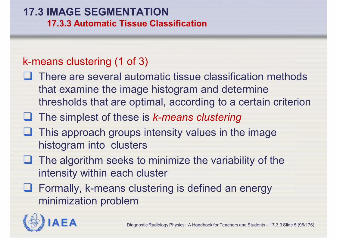
There are several automatic tissue classification methods
that examine the image histogram and determine
thresholds that are optimal, according to a certain criterion
The simplest of these is k-means clustering
This approach groups intensity values in the image
histogram into clusters
The algorithm seeks to minimize the variability of the
intensity within each cluster
Formally, k-means clustering is defined an energy
minimization problem
Diagnostic Radiology Physics: A Handbook for Teachers and Students – 17.3.3 Slide 5 (95/176)

IAEA
17.3 IMAGE SEGMENTATION 17.3.3 Automatic Tissue Classification
k-means clustering (2 of 3)
where
• αi is the cluster to which the pixel is assigned
• N is the number of pixels in the image
• Iq is the intensity of the pixel q
• µj is the mean of the cluster j , i.e., the average intensity of all
pixels assigned the label j
is read as “the point in the domain Ω where
the function f(x) attains its minimum”
Diagnostic Radiology Physics: A Handbook for Teachers and Students – 17.3.3 Slide 6 (96/176)
1
* * 2
1 [1 ]
1 :
arg min ( ) ,N
q
k
N k q j
j q j
Iα αα
α α µ… ∈ …= =
… = −∑ ∑
arg min ( )x
f x∈Ω

IAEA
17.3 IMAGE SEGMENTATION 17.3.3 Automatic Tissue Classification
k-means clustering (3 of 3)
Theoretically, the optimization problem is intractable
• but a simple iterative approach yields good approximations of the
global minimum in practice
This iterative approach requires the initial means of the
clusters to be specified
One of the drawbacks of k-means clustering is that it can
be sensitive to initialization
Diagnostic Radiology Physics: A Handbook for Teachers and Students – 17.3.3 Slide 7 (97/176)

IAEA
17.3 IMAGE SEGMENTATION 17.3.3 Automatic Tissue Classification
Example of segmentation by k-means clustering
Diagnostic Radiology Physics: A Handbook for Teachers and Students – 17.3.3 Slide 8 (98/176)
A slice from a brain
MRI
Partitioning of the image
histogram into clusters
based on initial cluster
means
Partitioning of the
histogram into clusters
after 10 iterations
Segmentation of the
image into gray
matter (GM), white
matter (WM) and
cerebrospinal fluid
(CSF)

IAEA
17.3 IMAGE SEGMENTATION 17.3.3 Automatic Tissue Classification
Fuzzy c-means clustering
In fuzzy c-means clustering, cluster membership is not
absolute
Instead, fuzzy set theory is used to describe partial cluster
membership
This results in segmentations where uncertainty can be
adequately represented
Diagnostic Radiology Physics: A Handbook for Teachers and Students – 17.3.3 Slide 9 (99/176)

IAEA
17.3 IMAGE SEGMENTATION 17.3.3 Automatic Tissue Classification
Gaussian mixture modelling (1 of 3)
Gaussian mixture modelling assumes that the pixel
intensities in an image are samples from a random
variable X with a probability density function f(x) that is a
weighted sum of n Gaussian probability densities, with
respective weights
where
• z is the standard normal distribution
• are unknown
Diagnostic Radiology Physics: A Handbook for Teachers and Students – 17.3.3 Slide 10 (100/176)
, ,i Nx x…
1,..., nα α
1
, , )( ; ) (k
mm m m m
m m
xzf x
µα µ σ α
σ=
−= ∑
, ,m m mα µ σ

IAEA
17.3 IMAGE SEGMENTATION 17.3.3 Automatic Tissue Classification
Gaussian mixture modelling (2 of 3)
The expectation-minimization algorithm (EM) is used to
find the maximum likelihood estimate of
Intuitively, Gaussian mixture modelling fits the image
histogram with a weighted sum of Gaussian densities
Once the optimal parameters have been found, the
probability that pixel belongs to a tissue class is found as
Diagnostic Radiology Physics: A Handbook for Teachers and Students – 17.3.3 Slide 11 (101/176)
* * *
1 , , , , 1
, , arg max ( , , ; , , ) arg max ( ; , , )m m m m m m
n
m m m N m m m i m m m
i
P x x f xα µ σ α µ σ
α µ σ α µ σ α µ σ=
= … = ∏
, ,m m mα µ σ
|( ) ( ).j m
j j
m
xm x zP L
µ
σ
−= =

IAEA
17.3 IMAGE SEGMENTATION 17.3.3 Automatic Tissue Classification
Gaussian mixture modelling (3 of 3)
Like fuzzy c-means, Gaussian mixture modelling can
describe uncertainty
For each tissue class, a probability image is generated
• estimating the probability that a given pixel belongs to a given
tissue class
It is possible to model partial volume effects
• for example, a pixel may be assigned 0.5 probability of being white
matter, 0.4 probability of being gray matter and 0.1 probability of
being CSF
• which can be interpreted as a partial volume effect, i.e., both white
matter and gray matter tissues present in the pixel
Diagnostic Radiology Physics: A Handbook for Teachers and Students – 17.3.3 Slide 12 (102/176)

IAEA
17.3 IMAGE SEGMENTATION 17.3.3 Automatic Tissue Classification
Example of segmentation using Gaussian mixture models
The mixture model (black curve) is a weighted sum of
three Gaussian probability densities, one for each tissue
type (red, blue and yellow curves)
Diagnostic Radiology Physics: A Handbook for Teachers and Students – 17.3.3 Slide 13 (103/176)
A mixture model
fitted to the
histogram of brain
MRI image
CSF probability
map generated
by the method
Grey matter
probability map
generated by the
method
White matter
probability map
generated by the
method

IAEA
17.3 IMAGE SEGMENTATION 17.3.3 Automatic Tissue Classification
Improving the performance of Gaussian mixture modelling
The performance of Gaussian mixture modelling can be
further improved by introducing constraints on consistency
of the segmentation between neighbouring pixels
Methods that combine Gaussian mixture modelling with
such spatial regularization constraints are among the most
widely used in brain tissue segmentation from MRI
Diagnostic Radiology Physics: A Handbook for Teachers and Students – 17.3.3 Slide 14 (104/176)

IAEA
17.3 IMAGE SEGMENTATION17.3.4 ACTIVE CONTOUR SEGMENTATION METHODS
Diagnostic Radiology Physics: A Handbook for Teachers and Students – 17.3.4 Slide 1 (105/176)

IAEA
17.3 IMAGE SEGMENTATION 17.3.4 Active Contour Segmentation Methods
Active contours
The term active contours is used to describe a family of image
segmentation algorithms
• emerged from the seminal work of Kass and Witkin (1988) on active
snakes
Before active snakes, the mainstream approach to object
segmentation involved edge detection, followed by linking edges to
form object boundaries
Such a deterministic approach is limited to simple segmentation
problems
Active snakes were a radical shift from the deterministic paradigm
• an early example of knowledge-based image analysis, where prior
knowledge about the shape and smoothness of object boundaries is used
to guide segmentation
Diagnostic Radiology Physics: A Handbook for Teachers and Students – 17.3.4 Slide 2 (106/176)

IAEA
17.3 IMAGE SEGMENTATION 17.3.4 Active Contour Segmentation Methods
Object segmentation
Unlike automatic tissue classification, active contour
methods address the problem of object segmentation
The goal is to identify a specific anatomical structure, or
small set of structures, in a biomedical image
The structure is represented by a contour (a closed curve
in 2D, or a closed surface in 3D)
The goal is to find a contour C that minimizes an energy
function E(C)
Diagnostic Radiology Physics: A Handbook for Teachers and Students – 17.3.4 Slide 3 (107/176)

IAEA
17.3 IMAGE SEGMENTATION 17.3.4 Active Contour Segmentation Methods
Minimising the energy function
The energy function typically comprises of two terms
• a term that measures how well the contour coincides with the
boundaries of objects in the image
• a term that measures how simple the contour C is
As an example, consider the 2D contour energy function
proposed by Caselles et al. (1997)
Diagnostic Radiology Physics: A Handbook for Teachers and Students – 17.3.4 Slide 4 (108/176)
1
0
1( ) where( ( )) ( ) d ( , )
( )( ,
1 | ) | I IC t C t t x y
G IE C g
x yg
σ
′ =∇
=+∫
o

IAEA
17.3 IMAGE SEGMENTATION 17.3.4 Active Contour Segmentation Methods
2D contour energy function
The contour C is parameterized by the variable
The function gI is called the speed function
• it is a monotonically decreasing function of the image gradient
magnitude
• it has very small values along the edges of I, and is close to 1
away from the edges of I
It is easy to verify that the energy E(C) is decreased by
• making C fall on edges in I, where gI is reduced
• making C shorter, which reduces
Diagnostic Radiology Physics: A Handbook for Teachers and Students – 17.3.4 Slide 5 (109/176)
1
0
1( ) where( ( )) ( ) d ( , )
( )( ,
1 | ) | I IC t C t t x y
G IE C g
x yg
σ
′ =∇
=+∫
o
, 0 1t t≤ ≤
( )C t′

IAEA
17.3 IMAGE SEGMENTATION 17.3.4 Active Contour Segmentation Methods
Evolution equation
Active contour methods are usually described not in terms
of the energy function E(C), but instead, in terms of an
evolution equation
where
• F is a scalar function of the image and the contour
• is the unit normal vector to C
This equation describes how to evolve the contour over
time T such that the energy E(C) decreases
Diagnostic Radiology Physics: A Handbook for Teachers and Students – 17.3.4 Slide 6 (110/176)
CF N
T
∂=
∂
r
Nr

IAEA
17.3 IMAGE SEGMENTATION 17.3.4 Active Contour Segmentation Methods
Deriving the evolution equation
The evolution equation and the function F can be derived
from the energy function using the calculus of variations
Different active contour methods use different functions F,
which correspond to different energy functions
• for example, the evolution equation for the 2D Caselles energy
function has the form
where κ is the curvature of the contour C
The same equation is used to describe contour evolution
in 3D, except that is used to describe the mean curvature
of the surface
Diagnostic Radiology Physics: A Handbook for Teachers and Students – 17.3.4 Slide 7 (111/176)
( )·I I
Cg g N N
Tκ − ∇
∂=
∂
r r

IAEA
17.3 IMAGE SEGMENTATION 17.3.4 Active Contour Segmentation Methods
Boundary representation for active contours (1 of 3)
In early active contour methods, the segmentation was
represented using a geometric boundary representation
• i.e. a piecewise cubic curve for 2D segmentation
• a surface for 3D segmentation
In modern active contour methods, the level set
representation is used instead, because of its numerical
stability and simplicity
The evolution equation can be adapted to the level set
representation
Diagnostic Radiology Physics: A Handbook for Teachers and Students – 17.3.4 Slide 8 (112/176)

IAEA
17.3 IMAGE SEGMENTATION 17.3.4 Active Contour Segmentation Methods
Boundary representation for active contours (2 of 3)
If φ is a function on , such that
• i.e. C is the zero level set of φ
Then the evolution equation can be rewritten in terms of φas
For instance, for the Caselles energy, the level set
evolution equation has the form
Diagnostic Radiology Physics: A Handbook for Teachers and Students – 17.3.4 Slide 9 (113/176)
n : ( ) 0nC φ= ∈ =x x
/ T Fφ φ∂ ∂ = ∇
divI Ig gT
φ φ φφ
φ φ
∂ ∇ ∇= + ∇ ∇ ∂ ∇ ∇

IAEA
17.3 IMAGE SEGMENTATION 17.3.4 Active Contour Segmentation Methods
Boundary representation for active contours (3 of 3)
The level set representation of the active contour has a
number of advantages
• level set methods are numerically robust and simple to implement
• with the level set representation, the topology of the segmentation
can change: multiple contours can merge into a single contour
• because the active contour is represented as a level set, the
contour is always a closed manifold
Diagnostic Radiology Physics: A Handbook for Teachers and Students – 17.3.4 Slide 10 (114/176)

IAEA
17.3 IMAGE SEGMENTATION 17.3.4 Active Contour Segmentation Methods
Active contours and tissue classification
Active contour segmentation can be used in conjunction with
automatic tissue classification
• using a method developed by Zhu and Yuille (1996)
This method uses the following definition for F
where
• and are the probabilities that a pixel at
position x belongs to the object of interest or to the background,
respectively
• these probabilities can be estimated from the image I using automatic
tissue classification or manual thresholding
• the constants α and β are user-specified weights that provide a trade-off
between the terms in the speed function
Diagnostic Radiology Physics: A Handbook for Teachers and Students – 17.3.4 Slide 11 (115/176)
[ ]) log ( Object) log ( Background)(F P Pα β κ= ∈ − ∈ −x x x
( Object)P ∈x ( Background)P ∈x

IAEA
17.3 IMAGE SEGMENTATION 17.3.4 Active Contour Segmentation Methods
Interpretation of evolution for tissue classification
The evolution has a very intuitive interpretation
The component of the force weighted by α• pushes the contour outwards if it lies inside of the object
• i.e.
• pushes the contour inwards if it lies outside of the object
The component -βκ
• pushes the contour inward at points with large negative curvature
• pushes it outwards at points with large positive curvature
The effect is to smooth out the sharp corners in the
contour, keeping the shape of the contour simple
Diagnostic Radiology Physics: A Handbook for Teachers and Students – 17.3.4 Slide 12 (116/176)
( Object) ( Background)P P∈ > ∈x x

IAEA
17.3 IMAGE SEGMENTATION 17.3.4 Active Contour Segmentation Methods
Active contours and segmentation
Regardless of the flavour of the active contour method, the
segmentation proceeds as follows
• the user provides an initial segmentation: for example, a circle or
sphere placed inside the object of interest
• contour evolution is then simulated by repeatedly applying the
evolution equation
• evolution is repeated
• until convergence
• or until the user interrupts it
Diagnostic Radiology Physics: A Handbook for Teachers and Students – 17.3.4 Slide 13 (117/176)

IAEA
17.3 IMAGE SEGMENTATION 17.3.4 Active Contour Segmentation Methods
Example of active contour segmentation
In the probability map white pixels have high object probability; blue
points have high background probability
Simple thresholding of the probability map will lead to a very noisy
segmentation
Diagnostic Radiology Physics: A Handbook for Teachers and Students – 17.3.4 Slide 14 (118/176)
An axial slice from
a low-contrast CT
volume
A map of
computed using
tissue classification
Initialization of the
active contour
method using five
spherical seeds
Segmentation after
1000 iterations of
evolution. Note that
the contours have
merged to form a
single surface
( Object) ( Background)P P∈ − ∈x x

IAEA
17.3 IMAGE SEGMENTATION 17.3.4 Active Contour Segmentation Methods
Extensions to active contour segmentation
Active contour segmentation is an area of active research
Numerous extensions to the methods have been proposed
in the recent years, including
• more general shape priors
• constraints on the topology of the segmentation
• various application-specific image-based criteria
Diagnostic Radiology Physics: A Handbook for Teachers and Students – 17.3.4 Slide 15 (119/176)

IAEA
17.3 IMAGE SEGMENTATION17.3.5 ATLAS-BASED SEGMENTATION
Diagnostic Radiology Physics: A Handbook for Teachers and Students – 17.3.5 Slide 1 (120/176)

IAEA
17.3 IMAGE SEGMENTATION 17.3.5 Atlas-Based Segmentation
Atlas-based segmentation (1 of 2)
Deformable image registration is a technique that
• automatically finds correspondences between pairs of images
• in recent years, has also become a popular tool for automatic
image segmentation
Perform registration between
• one image, called the atlas, in which the structure of interest has
been segmented, say manually
• another image I, in which we want to segment the structure of
interest
Diagnostic Radiology Physics: A Handbook for Teachers and Students – 17.3.5 Slide 2 (121/176)

IAEA
17.3 IMAGE SEGMENTATION 17.3.5 Atlas-Based Segmentation
Atlas-based segmentation (2 of 2)
By performing registration between the image and the
atlas
• we obtain a mapping φ(x) that maps every point in the image into a
corresponding point in the atlas
• this mapping can be used to transform the segmentation from the
atlas into image I
The quality of the segmentation is limited only by the
quality of the registration
Diagnostic Radiology Physics: A Handbook for Teachers and Students – 17.3.5 Slide 3 (122/176)

IAEA
17.3 IMAGE SEGMENTATION 17.3.5 Atlas-Based Segmentation
Example of atlas-based segmentation
Diagnostic Radiology Physics: A Handbook for Teachers and Students – 17.3.5 Slide 4 (123/176)
A brain MR image
used as the atlas
Manual
segmentation
of the
hippocampus
in the atlas
The target
image, in which
we want to
segment the
hippocampus
The atlas-
based
segmentation
of the target
image, overlaid
on the target
image
Atlas warped to
the target image
using
deformable
registration

IAEA
17.3 IMAGE SEGMENTATION 17.3.5 Atlas-Based Segmentation
Multiple atlas-based segmentation
Several authors have extended this simple idea to using
multiple atlases
Each atlas is registered to the image I, and segmentation
from each atlas is mapped into I
Because of registration errors, these warped
segmentations do not overlap perfectly
A voting scheme is used to derive a consensus
segmentation from
Diagnostic Radiology Physics: A Handbook for Teachers and Students – 17.3.5 Slide 5 (124/176)
1 KS S…
1 KS S…

IAEA
17.3 IMAGE SEGMENTATION 17.3.5 Atlas-Based Segmentation
Advantages of atlas-based segmentation
The appeal of atlas-based segmentation is that it is very
easy to implement
Several image registration software applications are
available in the public domain
All that the user needs to perform atlas-based
segmentation is an image, or several images, where the
object of interest has been manually segmented
Atlas-based segmentation can be applied in various
imaging modalities
• but its quality may not be as high as methods that use shape priors
Diagnostic Radiology Physics: A Handbook for Teachers and Students – 17.3.5 Slide 6 (125/176)

IAEA
17.4 IMAGE REGISTRATION17.4
Diagnostic Radiology Physics: A Handbook for Teachers and Students – 17.4 Slide 1 (126/176)

IAEA
17.4 IMAGE REGISTRATION 17.4
Image registration
Often in medical image analysis, we have to process
information from multiple images
• images with different modalities (CT, PET, MRI) from the same
subject
• images acquired at different time points from a single subject
• images of the same anatomical regions from multiple subjects
In all these, and many other situations, we need a way to
find and align corresponding locations in multiple images
Image registration is a field that studies optimal ways to
align and normalise images
Diagnostic Radiology Physics: A Handbook for Teachers and Students – 17.4 Slide 2 (127/176)

IAEA
17.4 IMAGE REGISTRATION 17.4
Image registration and transformations
Image registration is the problem of finding transformations
between images
Given an image I :Ω ϵ Rn → R and an image J :Ω ϵ Rn → R
Seek a transformation
• such that I(x) and J(φ(x)) are “similar” for all x in Ω
The meaning of “similar” depends on the application
• in the context of medical image analysis, “similar” usually means
“describing the same anatomical location”
• however, in practice such anatomical similarity cannot be
quantified, and “similar” means “having similar image intensity
features”
Diagnostic Radiology Physics: A Handbook for Teachers and Students – 17.4 Slide 3 (128/176)
:φ Ω → Ω

IAEA
17.4 IMAGE REGISTRATION 17.4
Characterisation of image registration problems
There are many different types of image registration
problems
They can be characterized by two main components
• the transformation model
• the similarity metric
Diagnostic Radiology Physics: A Handbook for Teachers and Students – 17.4 Slide 4 (129/176)

IAEA
17.4 IMAGE REGISTRATION 17.4
Image Registration
17.4.1 Transformation Models
17.4.2 Registration Similarity Metrics
17.4.3 The General Framework for Image Registration
17.4.4 Applications of Image Registration
Diagnostic Radiology Physics: A Handbook for Teachers and Students – 17.4 Slide 5 (130/176)

IAEA
17.4 IMAGE REGISTRATION17.4.1 TRANSFORMATION MODELS
Diagnostic Radiology Physics: A Handbook for Teachers and Students – 17.4.1 Slide 1 (131/176)

IAEA
17.4 IMAGE REGISTRATION 17.4
Image Registration
17.4.1 Transformation Models
17.4.2 Registration Similarity Metrics
17.4.3 The General Framework for Image Registration
17.4.4 Applications of Image Registration
Diagnostic Radiology Physics: A Handbook for Teachers and Students – 17.4.1 Slide 2 (132/176)

IAEA
17.4 IMAGE REGISTRATION 17.4.1 Transformation Models
Linear vs. non-linear transformations
The transformation can take many forms
The transformation is called linear when it has the form
where
• A is an n × n matrix
• b is an n × 1 vector
Otherwise, the transformation is non-linear
Diagnostic Radiology Physics: A Handbook for Teachers and Students – 17.4.1 Slide 3 (133/176)
( ) A bφ = +x x

IAEA
17.4 IMAGE REGISTRATION 17.4.1 Transformation Models
Rigid vs. non-rigid transformations
A special case of linear transformations are rigid
transformations
The matrix in rigid transformations is a rotation matrix
Rigid transformations describe rigid motions
They are used in applications when the object being
imaged moves without being deformed
Non-rigid linear transformations, as well as non-linear
transformations, are called deformable transformations
Diagnostic Radiology Physics: A Handbook for Teachers and Students – 17.4.1 Slide 4 (134/176)

IAEA
17.3 IMAGE SEGMENTATION 17.4.1 Transformation Models
Examples of spatial transformations
Diagnostic Radiology Physics: A Handbook for Teachers and Students – 17.4.1 Slide 5 (135/176)
Original image Image transformed
by rigid
transformation
(rotation and
translation)
Image
transformed by
linear affine
transformation
Image transformed
by non-linear
deformable
transformation

IAEA
17.4 IMAGE REGISTRATION 17.4.1 Transformation Models
Parametric transformations
Non-linear transformations can be parametric or non-
parametric
Parametric transformations have the form
where
• fi (x) :Ω → R is a basis, such as the Fourier basis or the B-spline
basis
• e1, e2 are unit vectors in the cardinal coordinate directions
• are the coefficients of the basis functions
Diagnostic Radiology Physics: A Handbook for Teachers and Students – 17.4.1 Slide 6 (136/176)
1 21 2
1
( ) ( ) ( )n
i i i i
i
W f e W f eφ=
= + + +…∑x x x x
1 2,
i iW W

IAEA
17.4 IMAGE REGISTRATION 17.4.1 Transformation Models
Parametric vs. non-parametric transformations
Usually, a relatively small number of low-frequency basis
functions is used to represent a parametric transformation
The resulting transformations vary smoothly across Ω
Such transformations are called low-dimensional non-
linear transformations
Non-parametric transformations do not have such a
parametric form
Instead, at every point in Ω, a vector v(x) is defined, and
the transformation is simply given by
Diagnostic Radiology Physics: A Handbook for Teachers and Students – 17.4.1 Slide 7 (137/176)
( ) ( )φ = +x x v x
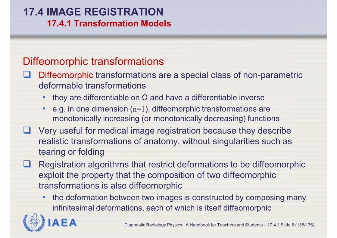
IAEA
17.4 IMAGE REGISTRATION 17.4.1 Transformation Models
Diffeomorphic transformations
Diffeomorphic transformations are a special class of non-parametric
deformable transformations
• they are differentiable on Ω and have a differentiable inverse
• e.g. in one dimension (n=1), diffeomorphic transformations are
monotonically increasing (or monotonically decreasing) functions
Very useful for medical image registration because they describe
realistic transformations of anatomy, without singularities such as
tearing or folding
Registration algorithms that restrict deformations to be diffeomorphic
exploit the property that the composition of two diffeomorphic
transformations is also diffeomorphic
• the deformation between two images is constructed by composing many
infinitesimal deformations, each of which is itself diffeomorphic
Diagnostic Radiology Physics: A Handbook for Teachers and Students – 17.4.1 Slide 8 (138/176)

IAEA
17.4 IMAGE REGISTRATION17.4.2 REGISTRATION SIMILARITY METRICS
Diagnostic Radiology Physics: A Handbook for Teachers and Students – 17.4.2 Slide 1 (139/176)

IAEA
17.4 IMAGE REGISTRATION 17.4
Image Registration
17.4.1 Transformation Models
17.4.2 Registration Similarity Metrics
17.4.3 The General Framework for Image Registration
17.4.4 Applications of Image Registration
Diagnostic Radiology Physics: A Handbook for Teachers and Students – 17.4.2 Slide 2 (140/176)

IAEA
17.4 IMAGE REGISTRATION 17.4.2 Registration Similarity Metrics
Similarity metrics
Image registration tries to match places in images that are
similar
Since true anatomical similarity is not known, surrogate
measures based on image intensity are used
Many metrics have been proposed
We will only review three such metrics
• Mean squared intensity difference
• Mutual information
• Cross-correlation
Diagnostic Radiology Physics: A Handbook for Teachers and Students – 17.4.2 Slide 3 (141/176)

IAEA
17.4 IMAGE REGISTRATION 17.4.2 Registration Similarity Metrics
Mean squared intensity difference
The similarity is measured as difference in image intensity
The similarity of images I and J is given by
Simple to compute
Appropriate when anatomically similar places can reasonably be
expected to have similar image intensity values
Not appropriate for
• registration of images with different modalities
• MRI registration, because MRI intensity values are not consistent across
scans
Diagnostic Radiology Physics: A Handbook for Teachers and Students – 17.4.2 Slide 4 (142/176)
[ ]21
Sim( , | ) ( ) ( ( )) d| |
I J I Jφ φΩ
= −Ω ∫ x x x

IAEA
17.4 IMAGE REGISTRATION 17.4.2 Registration Similarity Metrics
Mutual information (1 of 3)
Very useful for multimodality image registration
A pair of images of the body are acquired with different
modalities
• in modality 1, bone may have intensity range 100-200 and soft
tissue may have range 10-20
• in modality 2, bone may have intensity between 3000 and 5000,
and soft tissue may have intensity between 10000 and 20000
The mean square intensity difference metric would return
very large values if these two images are aligned properly
Another metric is needed that does not directly compare
the intensity values
Diagnostic Radiology Physics: A Handbook for Teachers and Students – 17.4.2 Slide 5 (143/176)

IAEA
17.4 IMAGE REGISTRATION 17.4.2 Registration Similarity Metrics
Mutual information (2 of 3)
The mutual information metric is derived from information
theory
To compute mutual information between images I and J,
we treat the pairs of intensity values (Ik, Jk) as samples
from a pair of random variables X, Y
One such sample exists at each pixel
Mutual information is a measure of how dependent
random variables X and Y are on each other
Diagnostic Radiology Physics: A Handbook for Teachers and Students – 17.4.2 Slide 6 (144/176)

IAEA
17.4 IMAGE REGISTRATION 17.4.2 Registration Similarity Metrics
Mutual information (3 of 3)
Mutual information is given by
where
• p(x,y) is the joint density of X and Y
• p(x) is the marginal density of X, p(y) is the marginal density of Y
The marginal densities are estimated by the histograms of
the images I and J
The joint density is estimated by the two-dimensional joint
histogram of the images I and J
Diagnostic Radiology Physics: A Handbook for Teachers and Students – 17.4.2 Slide 7 (145/176)
( , )( , )log
( ) ( )
p x yp x y dxdy
p x p y
∫ ∫

IAEA
17.3 IMAGE SEGMENTATION 17.4.2 Registration Similarity Metrics
Illustration of the joint histogram used in the computation of
the mutual information metric
Diagnostic Radiology Physics: A Handbook for Teachers and Students – 17.4.2 Slide 8 (146/176)
Axial slice from an
MR image
Axial slice from
a PET image
aligned with
the MRI
Joint histogram
of the MR and
PET images
Joint histogram
of the MRI and
misaligned
PET slice
PET slice
rotated out of
alignment with
the MRI

IAEA
17.4 IMAGE REGISTRATION 17.4.2 Registration Similarity Metrics
Cross-correlation
The cross-correlation metric is computed as follows
• at each pixel index k, we compute the correlation coefficient
between the values of image I in a small neighbourhood of pixels
surrounding k, and the values of image J over the same
neighbourhood
• the correlation coefficients are summed up over the whole image
The cross-correlation metric is robust to noise because it
considers neighbourhoods rather than individual pixels
However, it is expensive in computation time
Diagnostic Radiology Physics: A Handbook for Teachers and Students – 17.4.2 Slide 9 (147/176)

IAEA
17.4 IMAGE REGISTRATION17.4.3 THE GENERAL FRAMEWORK FOR IMAGE
REGISTRATION
Diagnostic Radiology Physics: A Handbook for Teachers and Students – 17.4.3 Slide 1 (148/176)

IAEA
17.4 IMAGE REGISTRATION 17.4.3 The General Framework for Image Registration
General algorithmic framework for image registration
Diagnostic Radiology Physics: A Handbook for Teachers and Students – 17.4.3 Slide 2 (149/176)

IAEA
17.4 IMAGE REGISTRATION 17.4.3 The General Framework for Image Registration
General algorithmic framework – transformation φ
Usually, one of the images is designated as a reference
image and the other image is the moving image
Transformations are applied to the moving image, while
the reference image remains unchanged
The transformation φ is defined by some set of
parameters
• small set for linear registration
• bigger for parametric non-linear registration
• and very large for non-parametric non-linear registration
Diagnostic Radiology Physics: A Handbook for Teachers and Students – 17.4.3 Slide 3 (150/176)

IAEA
17.4 IMAGE REGISTRATION 17.4.3 The General Framework for Image Registration
General algorithmic framework – similarity metric
Some initial parameters are supplied
• usually these initial parameters correspond to the identity
transformation
The transformation is applied to the moving image
• this involves resampling and interpolation because the values of
φ(x) fall between voxel centres
The resampled image J(φ(x)) is compared to the reference
image I(x) using the similarity metric
• this results in a dissimilarity value
• registration seeks to minimize this dissimilarity value
Diagnostic Radiology Physics: A Handbook for Teachers and Students – 17.4.3 Slide 4 (151/176)

IAEA
17.4 IMAGE REGISTRATION 17.4.3 The General Framework for Image Registration
General algorithmic framework – regularization prior
In many registration problems, an additional term, called
the regularization prior, is minimized
This term measures the complexity of the transformation φ• favours smooth, regular transformations over irregular
transformations
• can be though of as an Occam’s razor prior for transformations
Diagnostic Radiology Physics: A Handbook for Teachers and Students – 17.4.3 Slide 5 (152/176)

IAEA
17.4 IMAGE REGISTRATION 17.4.3 The General Framework for Image Registration
General algorithmic framework – objective function value
Together, the dissimilarity value and the regularization
prior value are combined into an objective function value
The gradient of the objective function with respect to the
transformation parameters is also computed
Numerical optimization updates the values of the
transformation parameters so as to minimize the objective
function
Diagnostic Radiology Physics: A Handbook for Teachers and Students – 17.4.3 Slide 6 (153/176)

IAEA
17.4 IMAGE REGISTRATION17.4.4 APPLICATIONS OF IMAGE REGISTRATION
Diagnostic Radiology Physics: A Handbook for Teachers and Students – 17.4.4 Slide 1 (154/176)

IAEA
17.4 IMAGE REGISTRATION 17.4.4 Applications of Image Registration
Applications of Image Registration
There are many image analysis problems that require
image registration
Different problems require different transformation models,
and different similarity metrics
We can group medical image registration problems into
two general categories
• registration that accounts for differences in image acquisition
• registration that accounts for anatomical variability (image
normalisation)
Diagnostic Radiology Physics: A Handbook for Teachers and Students – 17.4.4 Slide 2 (155/176)

IAEA
17.4 IMAGE REGISTRATION 17.4.4 Applications of Image Registration
Registration that accounts for differences in image acquisition
In many biomedical applications, multiple images of the same subject
are acquired
• images may have completely different modalities (MRI vs. CT, CT vs.
PET, etc.)
• images may be acquired on the same piece of equipment using different
imaging parameters
• even when parameters are identical, the position of the subject in the
scanner may change between images
To co-analyse multiple images of the same subject, it is necessary to
match corresponding locations in these images
This is accomplished using image registration
Within this category, there are several distinct subproblems that
require different methodology
Diagnostic Radiology Physics: A Handbook for Teachers and Students – 17.4.4 Slide 3 (156/176)

IAEA
17.4 IMAGE REGISTRATION 17.4.4 Applications of Image Registration
Accounting for Subject’s Motion
When multiple images of a subject are acquired in a short
span of time, the subject may move
• for example, in fMRI studies, hundreds of scans are acquired
during an imaging session
To analyse the scans, they must first be aligned, so that
the differences due to subject motion are factored out
Motion correction typically uses image registration with
rigid transformation models
Simple image similarity metrics suffice
Diagnostic Radiology Physics: A Handbook for Teachers and Students – 17.4.4 Slide 4 (157/176)

IAEA
17.4 IMAGE REGISTRATION 17.4.4 Applications of Image Registration
Alignment of Multi-Modality 3D Images
Often information from different imaging modalities must be combined
for purposes of visualisation, diagnosis, and analysis
• for example, CT and PET images are often co-analysed, with CT providing
high-resolution anatomical detail, and PET capturing physiological
measures, such as metabolism
The images have very different intensity patterns
• so registration requires specialised image similarity metrics, such as
mutual information
Often rigid transformations suffice
• however, some modalities introduce geometric distortions to images and
low-dimensional parametric transformations may be necessary to align
images
Diagnostic Radiology Physics: A Handbook for Teachers and Students – 17.4.4 Slide 5 (158/176)

IAEA
17.4 IMAGE REGISTRATION 17.4.4 Applications of Image Registration
Alignment of 3D and 2D Imaging Modalities
Sometimes registration is needed to align a 2D image of the subject to
a 3D image
• this problem arises in surgical and radiotherapy treatment contexts
• a 3D scan is acquired and used to plan the intervention
• during the intervention, X ray or angiographic images are acquired and
used to ensure that the intervention is being performed according to the
plan
• corrections to the intervention are made based on the imaging
For this to work, image registration must accurately align images of
different dimensions and different modality
This is a challenging problem that typically requires the image
registration algorithm to simulate 2D images via data from the 3D
image
Diagnostic Radiology Physics: A Handbook for Teachers and Students – 17.4.4 Slide 6 (159/176)

IAEA
17.4 IMAGE REGISTRATION 17.4.4 Applications of Image Registration
Registration that Accounts for Anatomical Variability (Image
Normalisation)
The other major application of image registration is to
match corresponding anatomical locations
• in images of different subjects
• in images where the anatomy of a single subject has changed over
time
The term commonly used for this is image normalisation
Again, there are several different applications
Diagnostic Radiology Physics: A Handbook for Teachers and Students – 17.4.4 Slide 7 (160/176)

IAEA
17.4 IMAGE REGISTRATION 17.4.4 Applications of Image Registration
Cross-sectional morphometry (1 of 2)
Often we are interested in measuring how the anatomy of
one group of subjects differs from another
• in a clinical trial, we may want to compare the anatomy of a cohort
receiving a trial drug to the cohort receiving a placebo
We may do so by matching every image to a common
template image using image registration with non-linear
transformations
We may then compare the transformations from the
template to the images in one cohort to the
transformations to the images in the other cohort
Diagnostic Radiology Physics: A Handbook for Teachers and Students – 17.4.4 Slide 8 (161/176)

IAEA
17.4 IMAGE REGISTRATION 17.4.4 Applications of Image Registration
Cross-sectional morphometry (2 of 2)
Specifically, we may examine the Jacobian of each
transformation
The Jacobian of the transformation describes the local
change in volume caused by the transformation
If
• an infinitesimal region in the template has volume δV0,
• the transformation φ maps this region into a region of volume δV1
Then the ratio δV1 / δV0 equals the determinant of the
Jacobian of the transformation
Diagnostic Radiology Physics: A Handbook for Teachers and Students – 17.4.4 Slide 9 (162/176)

IAEA
17.4 IMAGE REGISTRATION 17.4.4 Applications of Image Registration
Longitudinal morphometry
We may acquire multiple images of a subject at different
time points when studying the effect on human anatomy of
• disease
• intervention
• aging
To measure the differences over time, we can employ
parametric or non-parametric deformable registration
Because the overall anatomy does not change extensively
between images, the regularisation priors and other
parameters of registration may need to be different than
for cross-sectional morphometry
Diagnostic Radiology Physics: A Handbook for Teachers and Students – 17.4.4 Slide 10 (163/176)

IAEA
17.5 OPEN-SOURCE TOOLS FOR IMAGE ANALYSIS17.5
Diagnostic Radiology Physics: A Handbook for Teachers and Students – 17.5 Slide 1 (164/176)

IAEA
17.5 OPEN-SOURCE TOOLS FOR IMAGE ANALYSIS 17.5
Open-source tools for image analysis
This section briefly reviews several mature image processing and
analysis tools that were available freely on the Internet at the time of
writing
The reader can experiment with the techniques described in this
chapter by downloading and running these tools
Most tools run on Apple and PC computers (with Linux and Windows
operating systems)
These are just of few of many excellent tools available to the reader
The Neuroimaging Informatics Tools and Resources Clearinghouse
(NITRC, http://www.nitrc.org) is an excellent portal for finding free
image analysis software
Diagnostic Radiology Physics: A Handbook for Teachers and Students – 17.5 Slide 2 (165/176)
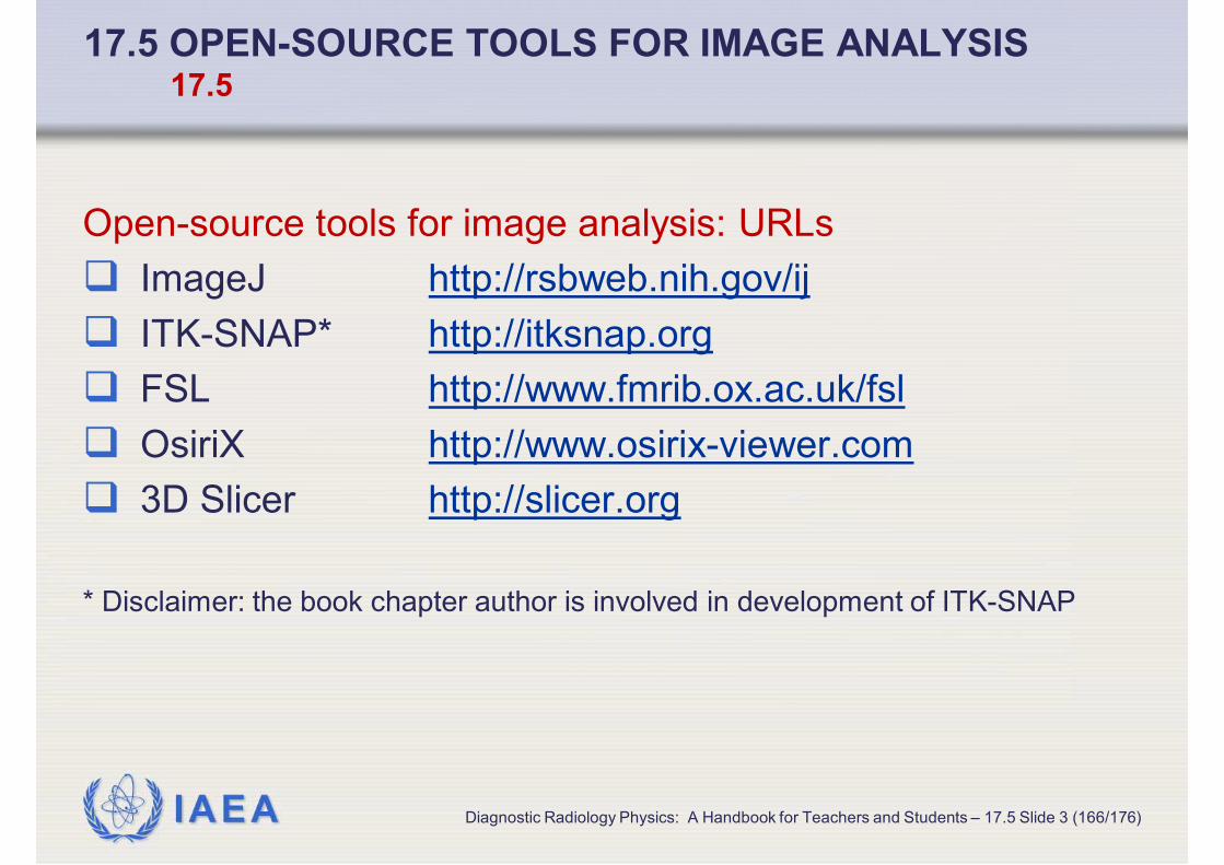
IAEA
17.5 OPEN-SOURCE TOOLS FOR IMAGE ANALYSIS 17.5
Open-source tools for image analysis: URLs
ImageJ http://rsbweb.nih.gov/ij
ITK-SNAP* http://itksnap.org
FSL http://www.fmrib.ox.ac.uk/fsl
OsiriX http://www.osirix-viewer.com
3D Slicer http://slicer.org
* Disclaimer: the book chapter author is involved in development of ITK-SNAP
Diagnostic Radiology Physics: A Handbook for Teachers and Students – 17.5 Slide 3 (166/176)

IAEA
17.5 OPEN-SOURCE TOOLS FOR IMAGE ANALYSIS 17.5
ImageJ
ImageJ provides a wide array of image processing
operations that can be applied to 2D and 3D images
In addition to basic image processing (filtering, edge
detection, resampling), ImageJ provides some higher-level
image analysis algorithms
ImageJ is written in Java
ImageJ can open many common 2D image files, as well as
DICOM format medical imaging data
Diagnostic Radiology Physics: A Handbook for Teachers and Students – 17.5 Slide 4 (167/176)

IAEA
17.5 OPEN-SOURCE TOOLS FOR IMAGE ANALYSIS 17.5
ITK-SNAP
ITK-SNAP is a tool for navigation and segmentation of 3D
medical imaging data
ITK-SNAP implements the active contour automatic
segmentation algorithms by Caselles et al. (1997) and Zhu
and Yuille (1996)
It also provides a dynamic interface for navigation in 3D
images
Several tools for manual delineation are also provided.
ITK-SNAP can open many 3D image file formats, including
DICOM, NIfTI and Analyze
Diagnostic Radiology Physics: A Handbook for Teachers and Students – 17.5 Slide 5 (168/176)

IAEA
17.5 OPEN-SOURCE TOOLS FOR IMAGE ANALYSIS 17.5
FSL
FSL is a software library that offers many analysis tools for
MRI brain imaging data
It includes tools for linear image registration (FLIRT), non-
linear image registration (FNIRT), automated tissue
classification (FAST) and many others
FSL supports NIfTI and Analyze file formats, among others
Diagnostic Radiology Physics: A Handbook for Teachers and Students – 17.5 Slide 6 (169/176)

IAEA
17.5 OPEN-SOURCE TOOLS FOR IMAGE ANALYSIS 17.5
OsiriX
OsiriX is a comprehensive PACS workstation and DICOM
image viewer
It offers a range of visualization capabilities and a built-in
segmentation tool
Surface and volume rendering capabilities are especially
well-suited for CT data
OsiriX requires an Apple computer with MacOS X
Diagnostic Radiology Physics: A Handbook for Teachers and Students – 17.5 Slide 7 (170/176)

IAEA
17.5 OPEN-SOURCE TOOLS FOR IMAGE ANALYSIS 17.5
3D Slicer
Slicer is an extensive software platform for image display
and analysis
It offers a wide range of plug-in modules that provide
automatic segmentation, registration and statistical
analysis functionality
Slicer also includes tools for image-guided surgery
Many file formats are supported
Diagnostic Radiology Physics: A Handbook for Teachers and Students – 17.5 Slide 8 (171/176)

IAEA
17. BIBLIOGRAPHY17.
Diagnostic Radiology Physics: A Handbook for Teachers and Students – 17. Bibliography Slide 1 (172/176)

IAEA Diagnostic Radiology Physics: A Handbook for Teachers and Students – 17. Bibliography Slide 2 (173/176)
17. BIBLIOGRAPHY17. Bibliography: Image Processing
DUDA, R., HART, P., Use of the Hough transformation to detect lines and
curves in pictures, Communications of the ACM 15 (1972) 11-15.
GONZALEZ, R.C., WOODS, R.E., EDDINS, S., Digital image processing
using MATLAB, Repr. with corr. [i.e. 3rd ] edn, Prentice Hall, Upper Saddle
River, NJ (2004) xvi, 716 pp.
LINDEBERG, T., Edge Detection and Ridge Detection with Automatic Scale
Selection, Int. J. Comput. Vision 30 (1998) 117-156.
PERONA, P., MALIK, J., Scale-Space and Edge Detection Using Anisotropic
Diffusion, IEEE T. Pattern Anal 12 (1990)

IAEA Diagnostic Radiology Physics: A Handbook for Teachers and Students – 17. Bibliography Slide 3 (174/176)
17. BIBLIOGRAPHY17. Bibliography: Image Segmentation (1 of 2)
CASELLES, V., KIMMEL, R., SAPIRO, G., Geodesic active contours, Int. J.
Comput. Vision 22 (1997) 61-79.
COLLINS, D.L., ZIJDENBOS, A.P. , KOLLOKIAN, V., SLED, J.G., KABANI,
N.J., HOLMES, C.J., EVANS, A.C. , Design and Construction of a Realistic
Digital Brain Phantom, IEEE Transactions on Medical Imaging, 17 (1998) 463-
468.
COOTES, T.F., TAYLOR, C.J., COOPER, D.H., GRAHAM, J., Active shape
models -- their training and application, Computer Vision and Image
Understanding 61 (1995) 38-59.
COOTES, T.F., EDWARDS, G.J., TAYLOR, C.J., Active Appearance Models,
IEEE Trans. Pattern Anal. Mach. Intell., IEEE Computer Society 23 (2001)
681-685.
KASS, M., WITKIN, A., TERZOPOULOS, D., Snakes: active contour models,
International Int. J. Comput. Vision 1 (1988) 321-331.
LI, S.Z., Markov Random Field Modeling in Image Analysis, 3rd edn, Springer
(2009).

IAEA Diagnostic Radiology Physics: A Handbook for Teachers and Students – 17. Bibliography Slide 4 (175/176)
17. BIBLIOGRAPHY17. Bibliography: Image Segmentation (2 of 2)
PHAM, D.L., XU, C., PRINCE, J.L., Current methods in medical image
segmentation, Annu Rev Biomed Eng 2 (2000) 315-37.
http://www.ncbi.nlm.nih.gov/entrez/query.fcgi?cmd=Retrieve&db=PubMed&do
pt=Citation&list_uids=11701515.
ZHU, S.C., YUILLE, A., Region Competition: Unifying Snakes, Region
Growing, and Bayes/MDL for Multiband Image Segmentation, IEEE Trans.
Pattern Anal. Mach. Intell., IEEE Computer Society 18 (1996) 884-900.

IAEA Diagnostic Radiology Physics: A Handbook for Teachers and Students – 17. Bibliography Slide 5 (176/176)
17. BIBLIOGRAPHY17. Bibliography: Image Registration
MAINTZ, J.B., VIERGEVER, M.A., A survey of medical image registration,
Med Image Anal 2 1 (1998) 1-36.
http://www.ncbi.nlm.nih.gov/entrez/query.fcgi?cmd=Retrieve&db=PubMed&do
pt=Citation&list_uids=10638851.
PLUIM, J.P., MAINTZ, J.B., VIERGEVER, M.A., Mutual-information-based
registration of medical images: a survey, IEEE transactions on medical
imaging 22 8 (2003) 986-1004.
http://www.ncbi.nlm.nih.gov/entrez/query.fcgi?cmd=Retrieve&db=PubMed&do
pt=Citation&list_uids=12906253.